
Abstract
Although crop yield generally responds positively to increased atmospheric CO2 concentration ([CO2]), the response depends on the species and environmental conditions. Thus, even though global [CO2] is increasing roughly uniformly, regional yield response to increased [CO2] will vary due to differences in climate and the mixture of crops. Although [CO2] effects have been shown to be important for economic and food security impacts of climate change, regional [CO2] effects are not often considered, and the few studies that have considered them disagree on regional patterns. Here regional yield effects of elevated [CO2] are examined by combining experimentally determined CO2 fertilization effect estimates with grid-level data on climate, crop areas, and yields. Production stimulation varies between regions, mostly driven by differences in climate but also by the mixture of crops. The variability in yield due to the variable response to elevated [CO2] is about 50–70% of the variability in yield due to the variable response to climate. There is, however, little agreement between studies regarding which regions benefit most from elevated [CO2]. This is likely because of interactions of CO2 with temperature, species, water status, and nitrogen availability, but no models currently account for all these interactions. These results suggest that regional differences in CO2 effects are of similar importance as regional differences in climate effects and should be included in models.
Export citation and abstract BibTeX RIS

Content from this work may be used under the terms of the Creative Commons Attribution 3.0 licence. Any further distribution of this work must maintain attribution to the author(s) and the title of the work, journal citation and DOI.
1. Introduction
Many studies have modeled the impact of climate change and elevated carbon dioxide ([CO2]) on regional and global food production. One consistent lesson from these studies, which have been conducted for more than twenty years, has been that the economic and food security impacts of climate change depend not only on the average global impact, but also on regional differences in impacts, which affect relative competitiveness for regionally or globally traded goods (Rosenzweig and Parry 1994, Hertel et al 2010).
These past studies have necessarily made some simplifying assumptions about the [CO2] fertilization effect (CFE) on crop yields. Some ignore the CFE altogether, which they justify because the study is focused only on the direct climate impacts (Lobell et al 2008) or because the CFE may be counteracted by factors such as pests and diseases not included in the crop models (Nelson 2009). Others, such as Rosenzweig and Parry (1994), assume a constant value of CFE that differs by crop but is applied equally to all locations. In either of these cases, regional differences in impacts for a given crop are driven mainly by climate, since both the CFE and atmospheric concentrations of [CO2] are spatially uniform.
However, a dependence of CFE on both crop species and soil moisture has been well established, and since both of these factors vary in space, so too should the CFE. In C3 species, elevated [CO2] stimulates carbon assimilation because the enzyme that fixes CO2, Rubisco, is not saturated at current atmospheric concentrations of CO2. Elevated [CO2] also inhibits oxygenation by Rubisco, which decreases losses of CO2 from photorespiration. However, C4 species already concentrate CO2 at the site of Rubisco. Thus, in C4 species, the carboxylation activity of Rubisco is already saturated at current concentrations of CO2, and photorespiration is essentially eliminated (Von Caemmerer and Furbank 2003), and increased atmospheric CO2 concentration does not increase carboxylation rate or decrease photorespiration. Many studies already account for differences in the response of C3 and C4 species to CO2, but they do not account for the fact that individual species may respond differently. Although using an average response for those two groups may work in some cases, studies find that the response of tuberous C3 species is large compared to other C3 species (Miglietta et al 1998, Bindi et al 2006, Högy and Fangmeier 2009, Ainsworth and McGrath 2010, Rosenthal et al 2012), thus warranting at least placing tuberous crops in a separate category if not treating each species individually.
Elevated [CO2] also decreases stomatal conductance in both C3 and C4 species (Ainsworth and Rogers 2007), which can result in decreased canopy water use (Leakey 2009), increased soil moisture content (Hunsaker et al 2000, Conley et al 2001, Leakey et al 2006), and potentially improved yield when water availability is low (Leakey et al 2004, Bernacchi et al 2007). Because C3 species benefit from increased carboxylation rate, decreased photorespiration, and improved water status, whereas C4 species benefit from only improved water status, C3 species on average tend to show stronger yield stimulation than C4 species (Ainsworth and Long 2005, Long et al 2006), and both types of plants show stronger yield stimulation in drought compared to well-watered environments (Prior and Rogers 1995, Ferris et al 1999, Ottman et al 2001, Schütz and Fangmeier 2001, Kang et al 2002, Mollah et al 2009, McGrath and Lobell 2011). Thus, because precipitation is variable spatially and temporally, and because different mixtures of crop species are grown in different regions, yield stimulation from elevated [CO2] will be temporally and spatially variable as well.
Some studies have used dynamical models that include physiological effects of CO2 and water availability to estimate crop responses to predicted future climate, and these models should be better at predicting crop responses on a regional basis. However, the estimates of the magnitude of the response are substantially different between studies, and the relative ranking of regions varies as well (tables 1 and 2). Furthermore, studies disagree on the degree of regional variability of CFE; some show less than two-fold differences in CFE between regions (Fischer 2009) while others show nearly three-fold differences (Müller et al 2010). These differences in variability of CFE alter conclusions about the relative importance of climate versus CO2 concentration on regional changes in yield, such that in some cases, changes in yield due to effects of climate are nearly 9 times more variable across regions than changes in yield due to effects of elevated [CO2] (Fischer 2009), whereas in other cases, changes in yield due to CO2 are slightly more variable across regions than changes due to climate (Müller et al 2010). Since there is no consensus, it is difficult to determine whether regional differences in the response of yield to elevated [CO2] should be included in studies and used to prioritize adaptation efforts.
Table 1. Carbon fertilization effect estimates from Müller et al (2010) normalized to a 100 ppm increase in [CO2].
| Region | CFE (%) |
|---|---|
| Africa | 9.9 |
| Centrally planned Asia | 11.6 |
| Europe | 10.3 |
| Former Soviet Union | 13.6 |
| Latin America | 13.1 |
| Middle East and North Africa | 8.4 |
| North America | 12.7 |
| Pacific OECD | 11.1 |
| Pacific Asia | 24.8 |
| South Asia | 24.2 |
Table 2. Carbon fertilization effect estimates from Fischer (2009) normalized to a 100 ppm increase in [CO2].
| Region | CFE (%) |
|---|---|
| North America | 3.6 |
| Europe | 4.2 |
| Russian Fed. | 3.7 |
| Central America & Carrib. | 2.5 |
| South America | 2.4 |
| Oceania and Polynesia | 2.4 |
| North Africa & West Asia | 3.6 |
| North Africa | 3 |
| West Asia | 3 |
| Sub-Saharan Africa | 2.4 |
| Eastern Africa | 3 |
| Middle Africa | 2.4 |
| Southern Africa | 1.8 |
| Western Africa | 2.4 |
| Asia | 3 |
| Southeast Asia | 2.4 |
| South Asia | 2.4 |
| East Asia and Japan | 3 |
| Central Asia | 3 |
The goal of the current study is to assess the importance of CO2 interactions on regional variation in CFE given differences in soil moisture and the mixture of crop species grown in different countries. We achieve this goal using a statistical model based on historical yield and weather data and experimental CFE estimates. This allows for the inclusion of some effects that current dynamical models do not seem to capture well, such as the unusually large response of tuber crops to elevated [CO2], and provides a largely independent estimate of regional changes for comparison with other studies. We focus on the CFE for a 100 ppm increase in [CO2], which corresponds to the increase expected between 2010 and 2040. Thus, we examine the degree to which regional disparities in CFE will drive regional differences in the combined impacts of climate change and [CO2] on crop productivity over the next few decades. The regional differences in CFE are also compared to regional differences in climate impacts taken from previous studies to gauge the relative importance of [CO2] in driving relative impacts. The results of this study are intended to complement studies that focus on impacts of changes in temperature and precipitation on crop yields, in particular those studies based on statistical models for which estimation of CO2 effects is very difficult (Schlenker and Roberts 2009, Schlenker and Lobell 2010, Lobell et al 2011).
2. Materials and methods
Data from experimental studies were used to create a relationship between moisture availability (represented by the ratio of growing season precipitation (P) to potential evapotranspiration (PET)) and CFE for several crop species (figure 1). Estimates of CFE in well watered and drought conditions were obtained from previous studies (table 3). Studies typically describe treatments as well watered or water stressed, and the actual P/PET in the studies used is unknown. Therefore, it was assumed that a P/PET of 1 is optimal and 0.5 is moderately water stressed. To account for the nonlinear response of CFE to water status, we assume a linear relationship for values less than 1 based on the line passing through the estimates at 0.5 and 1 P/PET. For values of P/PET 1 or greater, the CFE estimate at P/PET equal to 1 was used. Separate responses were calculated for different crops. For species for which there were no data, the response of a similar species was used. For crops that had an estimate in only a single water-status condition, the average slope of crops with available data was used to extrapolate to other values of P/PET.
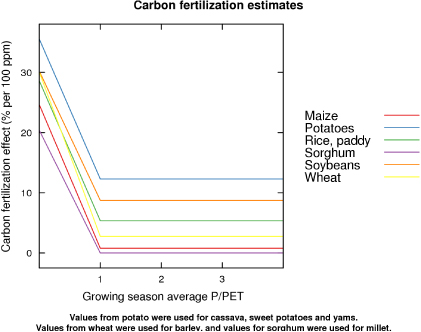
Figure 1. Carbon fertilization estimates for a 100 ppm increase in [CO2] for various species over a range of water-status conditions. These values were used with grid-cell level climate variable to estimate grid-level yield. Specific values and their sources are given in table 3.
Download figure:
Standard imageTable 3. Carbon fertilization effect (per cent increase per 1 ppm increase in carbon dioxide concentration) used in grid-cell estimates of yield. For crops without estimates, estimates for similar crop species were substituted. Footnotes are shown for only the unsubstituted species. CFEw and CFEd: Carbon fertilization effects at 1 and 0.5 P/PET respectively.
| Crop | Substitute | CFEw | CFEd | Slope |
|---|---|---|---|---|
| Barley | Wheat | 0.028 | 0.164 | −0.273 |
| Cassava | Potatoes | 0.123 | 0.244 | −0.242 |
| Maize | 0.008a | 0.127b | −0.239 | |
| Millet | Sorghum | −0.019 | 0.102 | −0.242 |
| Potatoes | 0.123c,d | 0.244 | −0.242e | |
| Rice, paddy | 0.054f,g | 0.175 | −0.242e | |
| Sorghum | −0.019h | 0.102h | −0.242 | |
| Soybeans | 0.087i | 0.195b | −0.215 | |
| Sweet potatoes | Potatoes | 0.123 | 0.244 | −0.242 |
| Wheat | 0.028j | 0.164j | −0.273 | |
| Yams | Potatoes | 0.123 | 0.244 | −0.242 |
aLeakey et al (2006). bMcGrath and Lobell (2011). cMiglietta et al (1998). dBindi et al (2006). eThis slope is the average slope of crops with CFE estimates in wet and dry conditions. fKim et al (2003). gYang et al (2006). hOttman et al (2001). iMorgan et al (2005). jManderscheid and Weigel (2007).
Since yield enhancement of elevated [CO2] responds nonlinearly to moisture availability, with benefits from greater water-use efficiency only occurring under dry conditions, using country-scale aggregate estimates of yield and water status will result in different yield stimulation estimates from those derived using gridded data. An approach with country-level data could over- or under-estimate yield stimulation depending on the spatial and temporal patterns of water status. To address this issue, and examine its potential consequences, country-level FAO data were disaggregated to a grid with the same resolution as the available water-status data.
In order to estimate yield on a 0.5° × 0.5° grid, a relationship was parameterized between gridded estimates of growing season water status and country-level yield data from 1961 to 2009 (step 1 in figure S1 available at stacks.iop.org/ERL/8/014054/mmedia), but some crop-country combinations were removed due to poor data (FAOSTAT; cf Mitchell and Jones 2005). Only data for crops that are not irrigated in a given country were used in the model. Crops were considered irrigated if either the percentage of irrigated agricultural area compared to total agricultural area or the percentage of total area equipped for irrigation compared to arable land and land under permanent crops exceeded 30% (FAOSTAT; the FAO definition of arable land is that which is under temporary crops, pasture or temporary fallow, not land potentially fit for agriculture). The measure of water status was P/PET, with PET calculated according to Thornthwaite (1948). For each country, average P/PET during the growing season was calculated by weighting the growing season P/PET in each cell by the area of crop harvested in that cell. In order to match the resolution of the climate data, estimates of harvested area (Monfreda et al 2008) were aggregated from 5' × 5' cells to 5° × 5° cells. Grid-level estimates of area harvested are only available for 2000, so for each country these estimates were scaled for each year such that the sum of all cells equaled the FAO estimate of area planted for that year. Growing season dates were determined from a crop planting and harvest data set (Sacks et al 2010). For each crop, yield was modeled with linear and quadratic parameters for P/PET and separate intercepts for each county. Using the coefficients for country-level growing season P/PET, yield was estimated in each grid cell (step 2 in figure S1 available at stacks.iop.org/ERL/8/014054/mmedia) using growing season P/PET in that cell with the constraint that the sum of production in all cells in a country for a single year must equal the FAO estimate of production in that country for that year. During cold periods with short day lengths, PET can have very small values, resulting in very large P/PET estimates, which can produce erroneous fits. To control for this, when fitting the model, only countries and years with a growing season average P/PET less than 5 were used (which removed less than 0.5% of the observations; excluded data can be found in table S1 available at stacks.iop.org/ERL/8/014054/mmedia) and when using the model to predict yield in these cells, P/PET was set to 5.
Historical data of CO2 concentrations (Keeling et al 2005) were used to adjust yield in each grid cell for a 100 ppm increase in atmospheric [CO2] and the magnitude of increase for each crop was based on the average growing season P/PET in the cell (step 3 in figure S1 available at stacks.iop.org/ERL/8/014054/mmedia). Since the purpose of this study is to determine the relative importance of CO2 interactions, the [CO2] increase is somewhat arbitrary but should reflect a realistic possibility, and 100 ppm was chosen as it is in line with lower IPCC projections of the increase in atmospheric [CO2] over 50 years. The total production of all crop species examined was calculated and the ratio of production in elevated [CO2] compared to historical conditions was determined. Because the number of calories produced may be more relevant than the quantity of production per se, the change in calorie production was estimated using the number of calories per mass from the USDA Standard Reference data set (Release 22; US Department of Agriculture, 2009).
3. Results and discussion
Values for CFE predicted using grid-cell estimates of P/PET were often higher than would be predicted from country-averaged estimates of growing season P/PET (figure 2), suggesting that calculations using aggregated yield data would likely under-estimate yield stimulation from elevated [CO2]. This occurs because CFE responds nonlinearly to P/PET, so using P/PET values that are averaged over too large an area can misestimate yield.

Figure 2. Country-level estimates of carbon fertilization effects for a 100 ppm increase in [CO2] for major crop species. Each point represents the mean carbon fertilization effect and mean growing season P/PET for all grid cells in a country in one growing season.
Download figure:
Standard imageYield response to elevated [CO2] shows considerable variability across regions, with values ranging from 5% to 17% increases in production for a 100 ppm increase of [CO2] averaged over regions (figure 3), 0%–33% for crops within regions (figure 4) and 1%–21% for individual countries (figure 5). Differences in climate resulted in large differences between regions, with dry areas showing a larger response than wet areas (figure 6B), except in the case of heavily irrigated regions such as the Middle East (figure 5). In addition, the mixture of crops impacts stimulation of production, with the production of more C3 crops relative to C4 crops being positively correlated with the increase of production in elevated [CO2] (figure 6A). In Russia, the response is particularly large because of the high production of potatoes, a tuberous species that shows a relatively strong response to elevated [CO2] (figures 1 and 6C).

Figure 3. Carbon fertilization effect for regions of the world averaged over the entire study period. Points are the estimate using the mean estimate of the carbon fertilization effect assuming a 100 ppm increase in atmospheric [CO2], and bars are estimates using the 95% upper and lower estimates of the carbon fertilization effect, derived from Long et al (2006).
Download figure:
Standard image
Figure 4. Carbon fertilization effect estimates for crops and regions of the world averaged over the entire study period. Points are the estimate using the mean estimate of the carbon fertilization effect assuming a 100 ppm increase in atmospheric [CO2], and bars are estimates using the 95% upper and lower estimates of the carbon fertilization effect, derived from Long et al (2006).
Download figure:
Standard image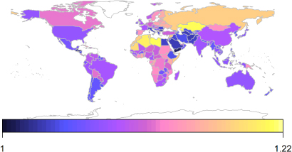
Figure 5. Carbon fertilization effect estimates for a 100 ppm increase in [CO2] for total production for countries of the world.
Download figure:
Standard image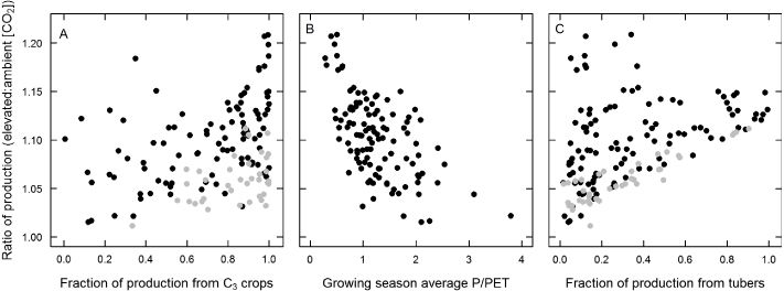
Figure 6. Carbon fertilization effect estimates for a 100 ppm increase in [CO2] plotted against factors that vary by region. Each point is the mean for all crops in a single country over the entire study period. Black points are for nonirrigated countries. Gray points are for irrigated countries.
Download figure:
Standard imageThe pattern of enhancement of calorie production is similar to crop production (figure 7). However, calorie production is not as strongly enhanced as crop production in almost the entire world, notably in many portions of Africa and South America, indicating that the majority of production that responds to elevated [CO2] is composed of crops that are less calorie dense, such as cassava and potato, for which yield is reported at a higher moisture content.
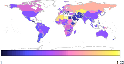
Figure 7. Carbon fertilization effect for a 100 ppm increase in [CO2] as a ratio of calories produced for countries of the world.
Download figure:
Standard imageUnderstanding regional yield responses to climate change will help countries prioritize agricultural improvement, so to determine whether there is consensus across studies, the results here were compared to findings from previous studies. For comparison with previous studies, CFE estimates were calculated using the same regions as Müller and Fischer, and CFE estimates from those studies were adjusted to a 100 ppm increase (tables 1 and 2). The CFE estimates here were intermediate to these two studies, with the mean CFE and coefficient of variation approximately 200% and 50% larger, respectively, than the estimates of Fischer and 33% and 30% smaller, respectively, than the estimates of Müller. The magnitude of response is substantially different among studies, with a 5–17% (this study), 2.4–4.2% (Fischer 2009) and 8–24% (Müller et al 2010) increase in yield per 100 ppm increase in [CO2].
The model used by Fischer (2009) uses a CFE based on CO2 concentration, photosynthesis type (C3 or C4) and temperature (cf Parry et al 2004). Although the model adjusts stomatal conductance for elevated CO2 concentration, it applies the same adjustment to all regions. Thus is may not fully simulate differences in regional responses to CO2 and is similar to using an average CFE across possible water statuses, but because the response of CFE to water status is nonlinear, this can lead to incorrect estimates. As shown here, that approach tends to underestimate CFE, which may explain the lower estimates of Fischer (2009). The magnitudes of the estimates here are slightly less than those of Müller et al (2010), who use a model of photosynthesis that responds to CO2 concentration, temperature and canopy conductance (Haxeltine and Prentice 1996). The model adjusts canopy conductance depending on water stress, and therefore the response of conductance will vary across regions. Since the interaction between CFE and water status is due to water saving from lower conductance, this approach produces CFE estimates that vary across regions. Their mechanistic approach and the empirical approach used here each have benefits and drawbacks and will likely produce somewhat different results from each other because they are based on different methods and data. However, the specific reasons for disagreement with this study are not as obvious as for Fischer (2009).
The coefficient of variation for CFE in this study is 50 and 70% of the coefficient of variation of climate effects in Müller and Fischer, respectively. Thus, regional differences in yield due to variation in CO2 response is at least on par with regional differences due to climate alone, which agrees with the findings of Müller, that regional differences due to CO2 and climate change combined are somewhat more variable than regional differences from climate alone.
To determine whether studies agree on which regions will be the most or least responsive, regardless of the absolute magnitude, the relative rankings of regions were also compared (figures 8 and 9). Compared to the results of Fischer (2009), the rankings are in general agreement. However, the comparison is somewhat noisy since the results in Fischer (2009) do not vary much across regions and were rounded to whole numbers, resulting in multiple tied ranks. One large difference between the two results is the response in the Sahel, which is one of the largest responders in this study, but a small responder in the study by Fischer (2009). This difference is likely due to the large production of cassava, and the large stimulation used for tuberous crops in this analysis, whereas Fischer (2009) only considers cereals. Compared to the results of Müller et al (2010), there is very little agreement (figure 9), and the rankings are nearly perfectly reversed, which means that even though the mean estimate is only slightly lower than the one of Müller et al (2010), the regions that are benefiting are different between studies. The difference is again likely due in part to the large response of tubers used in this study. However, one common finding in the three studies is the large response in Russia.

Figure 8. Comparison of the rank of carbon fertilization effect for regions in this study with the ranks of the same regions used by Fischer (2009). Regions are arranged by rank on the x axis from the smallest CFE (Central America and Caribbean) to the largest CFE (Russian Federation) based on estimates from this study. Values on the y axis are the rank of CFE as determined from Fischer (2009) when using current cultivars (red) or cultivars adapted to future climate in that region (blue). Points for the two estimates are slightly offset from whole numbers so they can be seen. Values given by Fischer (2009) are rounded results in multiple tied ranks. The dashed line represents where points would fall if the ranks were identical between the two studies.
Download figure:
Standard image
Figure 9. Comparison of the rank of carbon fertilization effect for regions in this study with the ranks of the same regions used by Müller et al (2010). Abbreviations are as follows and a list of countries included in each regions can be found in Müller et al (2010): AFR, Sub-Saharan Africa; CPA, Centrally-Planned Asia; EUR, Europe; FSU, Former Soviet Union; LAM, Latin America; MEA, Middle East-North Africa;, NAM, North America; PAO, Pacific OECD; PAS, Pacific Asia; SAS, South Asia. Regions are arranged by rank on the x axis from the smallest CFE (PAS) to the largest CFE (FSU) based on estimates from this study. Values on the y axis are the rank of CFE as determined from Müller et al (2010) when using the A1B (red) A2 (blue) or B1 (green) SRES emission scenarios. Points for the three estimates are slightly offset from whole numbers so they can be seen. The dashed line represents where points would fall if the ranks were identical between the two studies.
Download figure:
Standard imageThe proportion of tubers that make up production in a region had a strong influence on CFE in regions (figure 6C), and some regions would not have shown such a strong stimulation if tubers were not treated separately, e.g., the Sahel of Africa. Other studies find that production of cereal crops is projected to decrease in Africa (Parry et al 2005), but in some parts of Africa, cereals contribute less than 30% of calories in a diet, with tubers, such as cassava, providing nearly half of calories in some areas (Burke and Lobell 2010). For such regions, understanding the response of tubers to elevated CO2 will be critical for estimating impacts, but there are relatively few studies that examine yield response of tuberous species to elevated [CO2], many of those are chamber or glasshouse experiments, which may alter the yield response (Leakey 2009). However, recent results from a FACE experiment in the US Midwest found that dry mass of cassava tubers increased by 100% in CO2 concentration expected for midcentury (Rosenthal et al 2012, Rosenthal and Ort 2012), suggesting that the large response of tubers seen in enclosure studies is achievable in well-managed fields. Furthermore, even though there have been multiple studies in temperate, intensively managed systems, few of the previous experiments have been performed in conditions similar to the growing environments of developing counties, in which the response could be very different (Leakey et al 2012). This is particularly important for dry conditions, for which there are currently no studies, but which prevail in Africa where tuberous crops make up a large proportion of production. This study assumes that these species respond similarly to other species in dry climates, which is reasonable but experimentally unverified. Thus, even though those areas are some of the most important from a food security perspective, they still have large uncertainty. Therefore, reducing uncertainty in the yield response of tuberous species will be important for determining net impacts of elevated [CO2] and climate trends in Africa, but the necessary experiments have not be performed.
The ratios of P/PET used to estimate CFE in this study are based on historical weather, and therefore do not take account of future changes in climate. Projections indicate that dry areas are likely to become drier and wet areas will become wetter (Meehl et al 2007). Thus regional differences in relative yield stimulation are likely to be further exaggerated when considering future climate conditions compared to the estimates here.
In addition to the mixture of crops and moisture availability, another factor likely to cause regional variability in CFE is nitrogen (N) availability. For most species studied, CFE is larger when there are no N limitations, with a meta-analysis showing that CFE was twice as large in high N application treatments compared to low N treatments (Ainsworth and Long 2005). In most studies that examine CFE in different moisture conditions, N is not limiting, and thus the estimates used here are likely the maximum response that can be expected. Furthermore, because many of the dry regions are also regions where little N fertilizer is used, the actual CFE will likely be considerably smaller, suggesting that the response of yield in some places, such as many countries in Africa, could be half as large. As a consequence of rising atmospheric [CO2], the value of adding N fertilizer or growing N-fixing crops could be substantially increased in many places. That is, in addition to the yield benefit from added N, the crop could make better use of increased [CO2], assuming that the CO2-by-N interaction is similar in dry conditions. At the same time, higher N application rates are likely to increase the sensitivity of yields to warming and drought, because a reduction in nutrient stress allows plants to respond better in years with favorable climates (Schlenker and Lobell 2010). However, yield response to the interaction of [CO2], water status, species, and N availability is not well understood.
4. Conclusion
Although classifying crops into C3 or C4 species is likely acceptable for many species, it may not be appropriate for tuberous crops. Those species have a large response to elevated [CO2], resulting in the proportion of production from tubers strongly influencing yield stimulation in some regions in this study. More research is needed to determine whether such a large response is typical of all tuberous crops in a range of environments, particularly in dry conditions for which there are no estimates, but the current knowledge suggests that if estimates for individual species are not used, then tuberous species should at least be in a separate category.
For the interaction with water status, and other nonlinear interactions, the scale examined needs to be considered, or estimates will be incorrect. Ideally, the temporal and spatial resolution would be just fine enough so that none of the observations span nonlinear parts of the function. For example, in the case of water status, all P/PET values in a cell should be above or below 1. In practice, it is likely an impossible situation to avoid, so the scale should be chosen to minimize such effects rather than remove them. Since most useful functions are linear or nearly linear for portions of the function, there will be diminishing returns from using finer resolutions, but the results here suggest that country-level data may be insufficient for some factors, and finer scale data sets or disaggregation should be used if possible when dealing with nonlinear responses.
The variability of yield stimulation in response to [CO2] is nearly as large as variability due to climate, so, for estimating regional responses, understanding yield interactions with CO2 are likely equally as important as understanding yield response to climate itself, and models should try to include these interactions. More experiments examining the interactions between CO2 and drought would aid this, and experiments examining interactions between CO2 and temperature would be particularly useful since few have been conducted.
For global estimates, not including interactions between CO2 and other factors may not strongly affect results because some aspects will be overestimated and others will be underestimated, canceling each other out. At regional scales, however, it is more likely that failing to account for the interactions will result in estimating a change in the wrong direction. For instance, if a crop were growing at its optimum in current climate, and temperature and CO2 concentration increased slightly in the future, not accounting for the interaction would estimate a decline in yield, but including the interaction would estimate an increase. Because such scenarios require several things to happen simultaneously, and because these interactions are only a small part of complex models, it is likely that previous models that do not include interactions still provide valuable information overall, but may not capture all of the effects for certain regions. In terms of prioritization, regional effects are of primary importance and good estimates will be required for international organizations to target the neediest areas, and for local organizations to target the most effective adaptations. Thus, including realistic interactions of CO2 with the environment remains an important area of research for prioritization.
Acknowledgment
Funding for this work was provided by the Rockefeller Foundation.