

Abstract
In this study, we investigate the change in multi-day precipitation extremes in late winter in Europe using observations and climate models. The objectives of the analysis are to determine whether climate models can accurately reproduce observed trends and, if not, to find the causes of the difference in trends.
Similarly to an earlier finding for mean precipitation trends, and despite a lower signal to noise ratio, climate models fail to reproduce the increase in extremes in much of northern Europe: the model simulations do not cover the observed trend in large parts of this area. A dipole in the sea-level pressure trend over continental Europe causes positive trends in extremes in northern Europe and negative trends in the Iberian Peninsula. Climate models have a much weaker pressure trend dipole and as a result a much weaker (extreme) precipitation response.
The inability of climate models to correctly simulate observed changes in atmospheric circulation is also primarily responsible for the underestimation of trends in the Rhine basin. When it has been adjusted for the circulation trend mismatch, the observed trend is well within the spread of the climate model simulations. Therefore, it is important that we improve our understanding of circulation changes, in particular related to the cause of the apparent mismatch between observed and modeled circulation trends over the past century.
Export citation and abstract BibTeX RIS

Content from this work may be used under the terms of the Creative Commons Attribution 3.0 licence. Any further distribution of this work must maintain attribution to the author(s) and the title of the work, journal citation and DOI.
1. Introduction
Estimates of future changes in extremes of multi-day precipitation sums are critical for estimates of future discharge extremes of large river basins and changes in frequency of major flooding events (Kew et al 2010). A correct representation of past changes is an important (but not sufficient) condition to have confidence in projections for the future.
High discharge rates for the Rhine in the Netherlands usually occur in (late) winter (Rijkswaterstaat Waterdienst 2012). Evaporation rates in winter are low and soils are often saturated and sometimes frozen. Rainfall has the potential to melt large amounts of snow by bringing large amounts of thermal energy to the snowpack, increasing runoff (Disse and Engel 2001). Over the past century the average (Disse and Engel 2001) and extreme (Wang et al 2005) discharge of the Rhine in winter increased. Model results project a further increase for the current century (e.g. Hurkmans et al 2010, Lenderink et al 2007, Kew et al 2010, te Linde et al 2010), mainly caused by an increase in precipitation (van Pelt et al 2012) and a shift of the snowmelt season from spring to winter (Barnett et al 2005).
The climate in Europe depends strongly on the atmospheric circulation. Western circulation brings moist air from the Atlantic to the continent (van Ulden and van Oldenborgh 2006), leading to increasing precipitation over the continent. In an earlier paper we concluded that a misrepresentation of circulation changes in climate models is responsible for the underestimation of increase in winter precipitation in northwest Europe over the past century in climate models (van Haren et al 2013). Recent research finds that higher quantiles of daily precipitation correlate well with mean precipitation (Benestad et al 2012) and that the increase in mean winter extreme precipitation in Europe is similar across a range of multi-day sums (Kew et al 2010). The inability of climate models to capture the observed trend in atmospheric circulation could, through transport of moisture, also influence trends in extreme precipitation: particular circulation types may be more favorable for extreme precipitation events to occur.
In this paper we investigate whether the spread of climate models (which includes natural variability) covers the observed increase in extreme precipitation in Europe and the Rhine basin in late winter. We evaluate modeled trends in extreme precipitation, and try to find causes for the difference in trends. We only consider the uncertainty in trends of extreme precipitation. Estimates of trends in river discharge requires the coupling with a hydrological model of the catchment area and hydraulic models of the river and its main branches (e.g. Lenderink et al 2007), which is outside the scope of this study.
2. Data and methods
2.1. Study area
We study the extreme precipitation in Europe and the Rhine area (indicated by the area in figure 1(a)). The Rhine is the longest river in western Europe, originating in the Swiss Alps. From Switzerland it flows through the principality of Liechtenstein, Austria, Germany and France before it enters the Netherlands near Lobith, on the Dutch–German border. The main flow reaches the sea near Rotterdam, the Netherlands. The drainage area of the Rhine is approximately 185 000 km2.
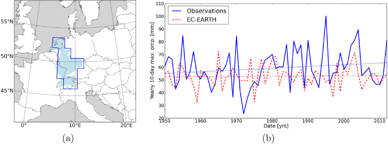
Figure 1. (a) Location and area of the Rhine basin within Europe. The light blue area indicates the actual catchment area. The dark blue line represents the grid box approximation used in this study. (b) Time-series (with accompanying trend estimates) of JFM annual maxima 10 day precipitation sums averaged over the Rhine basin (mm).
Download figure:
Standard imageNatural variability plays an important role in determining trends of extreme events. To give an impression of the magnitude of the inter-annual variability, we show in figure 1(b) the observed and modeled time-series (with accompanying trend estimates) of annual maxima January–March (JFM) 10 day running precipitation sums averaged over the Rhine basin. The modeled series is only shown for one climate model (EC-EARTH, 1 member). Strong inter-annual variability is found for both observed and modeled time-series, although with a larger (absolute) magnitude for the observed series.
In late winter precipitation in Europe is mainly caused by frontal systems from the Atlantic. The mean precipitation decreases from the coast and is highest on the west side of mountain ranges. The latitude where most rain falls is determined by the zonal pressure difference, with a blocking high over northern Europe causing dry weather there and more rain in southern Europe. Conversely, a stronger westerly flow brings more rain to northern Europe and less to the Mediterranean area.
2.2. Analysis period
Trends are computed from the annual maximum series of the 10 day running precipitation sums (RX10day) for the northern hemisphere late winter (JFM) 1950–2012 period. Extreme 10 day precipitation sums are an important statistic for extreme peak flows for the Rhine river in the Netherlands (e.g. Shabalova et al 2003). The choice for the late winter period is dictated by past discharge extremes of the river Rhine. More than 75% of winter annual discharge extremes (Rijkswaterstaat Waterdienst 2012) at the Lobith station (near the Dutch–German border) since 1950 occurred in the second half of the winter (JFM), despite slightly more (multi-day) extreme precipitation events in the river basin occurring in the first half of the winter.
The JFM period happens to coincide with the season of strongest observed and simulated trends in atmospheric circulation in this region. The late European winter has seen a change in circulation regime over the past century, related to an eastward extension of the belt of zonal winds (Haarsma et al 2013, Ulbrich et al 2008), that is outside the range of natural variability of model results (e.g. van Oldenborgh et al 2009, van Haren et al 2013).
2.3. Datasets
We use daily precipitation data in this study. The multi-model ensemble used in this study is obtained from the Coupled Model Intercomparison Project Phase 5 (CMIP5, Taylor et al 2011). The CMIP5 dataset consists of models at varying horizontal grid spacing, typically in the order of one hundred to a few hundreds of kilometers. For the period before 2005 we use the historic runs. For the period after 2005 we use the RCP4.5 experiment runs. We limit ourselves to use only historical runs that have a RCP4.5 extension. To not bias the results to models with more members available, we use only the first available member per model. The FGOALS-g2 model is omitted from this analysis due to inconsistencies between the daily and monthly precipitation fields. This brings the total number of models used in this study to 21 (EC-EARTH, HadGEM2-CC, HadGEM2-ES, CCSM4, GFDL-ESM2G, GISS-E2-R, MIROC-ESM-CHEM, NorESM1-M, BCC-CSM1-1, CNRM-CM5, GFDL-ESM2M, IPSL-CM5A-LR, MIROC5, MPI-ESM-LR, CanESM2, CSIRO-Mk3-6-0, IPSL-CM5A-MR, MIROC-ESM, MRI-CGCM3, INMCM4, ACCESS1-0). Different RCP scenarios are available, but for the short period after 2005 these are almost identical. All models are bilinearly interpolated on a regular 1.5° grid before analysis, resulting in 13 grid points for the Rhine area.
To evaluate the model results we use the state-of-the-art gridded high resolution (0.5°) precipitation fields of the European ENSEMBLES project version 7.0 (Haylock et al 2008, E-OBS). The observations are averaged to the same regular 1.5° grid when compared directly with the model results.
For validation of our results we also use the high resolution (25–50 km resolution) multi-model ensemble of regional climate models (RCMs) provided by Research Theme 2b of the European ENSEMBLES project (RT2b, van der Linden and Mitchell 2009). The RCMs are forced at their lateral boundaries by results from global climate models (GCMs) from the Coupled Model Intercomparison Project Phase 3 (CMIP3, Meehl et al 2007). There are no large differences between the results of CMIP3 and CMIP5 models over Europe. The RCM ensemble consists of a total of 18 RCM/GCM combinations.
3. Methodology
3.1. Effect of circulation change
To investigate if the change in mean circulation characteristics affects the change in precipitation extremes, we fit a simple statistical model that isolates the linear effect of mean circulation anomalies (van Ulden and van Oldenborgh 2006, van Oldenborgh et al 2009, van Haren et al 2013) to the anomalies of the annual maxima series of RX10day, P'(x,y,t). This is done for each dataset separately. These effects include the influence of mean geostrophic wind anomalies Ug(x,y,t),Vg(x,y,t) and vorticity anomalies  and the remaining noise η(x,y,t). The longitude and latitude of the grid box is indicated by (x,y),t indicates the time.


The geostrophic wind anomalies and vorticity anomalies are computed from the monthly NCEP/NCAR Reanalysis sea-level pressure (SLP) dataset (NCEP/NCAR, Kistler et al 2001) when considering observed precipitation anomalies, but other SLP datasets (Twentieth Century Reanalysis (20C, Compo et al 2011), Trenberth Northern Hemisphere SLP (Trenberth and Paolino 1980)) give similar results. Model SLP output is used in combination with modeled precipitation anomalies. The coefficients BW(x,y),BS(x,y),BV(x,y) and A(x,y) are fitted over 1950–2012 for each 3 month winter period.
3.2. Trend definition
Our approach is to fit a non-stationary generalized extreme value (GEV) distribution to the annual maxima series of RX10day, as well as separately to the derived circulation and residual components. The GEV distribution is described as (e.g. Katz et al 2002)
where μ,σ > 0, and γ are the location, scale and shape parameters, respectively. We adopted the homoscedastic model (constant variance) where the location parameter is described by

here μ1 is a trend in the location parameter, and t is a covariate linear in time from 1950–2012. Whenever we refer to a trend in precipitation extremes in later sections we refer to the trend as estimated by the μ1 parameter. The scale and shape parameters are constant in the homoscedastic model. Experiments allowing for a time-varying scale parameter produced similar trends in the location parameter.
The parameters are estimated by the maximum likelihood method because of its ability to estimate time dependent covariates as recommended by Katz et al (2002) and Kharin and Zwiers (2005).
3.3. Rank histograms
As an aggregated statistic for the performance of our model ensemble we compute rank histograms. A rank histogram is created by tallying the rank of the observation relative to values from the ensemble sorted from lowest to highest. If there are N ensemble members, there are N + 1 ranks, including the two outer edges, the observation could fall. A reliable ensemble produces a flat histogram. If the model ensemble has a trend bias, a larger part of the area lies at one end of the ensemble and that edge of the histogram curves up.
To investigate whether there is a significant deviation from a reliable ensemble, i.e., whether it is unlikely to be a fluctuation in the distribution of model spread and natural variability, the strong correlation between neighboring grid points needs to be taken into account. We do this by including the correlation as represented by the models in the ensemble when constructing significance intervals. The significance intervals are constructed by considering each model in turn to be the 'truth' (Annan and Hargreaves 2010) and computing its rank histogram with respect to the other models. The 90% confidence interval is then given by the distance between the second lowest and the second highest ranked member for each bin (using a 1-sided test to only account for trend biases and assuming the outcomes of all members are equally likely).
4. Modeled versus observed trends
Precipitation extremes in late winter have increased in the northern half of Europe in the last 60 years. In figure 2 we show the observed (a) and modeled (b) trend in 10 day annual maxima (RX10day) for late winter between 1950–2012. Externally forced changes should appear in the mean trend of the model ensemble (figure 2(b)). If no trend is found here, the observed trend is either caused by natural variability or climate models fail to (correctly) represent processes that are important for precipitation. The figures show that the average modeled trend in northern Europe is much weaker than the observed trend. The trend bias in the models is significant in northern Europe: figure 2(c) shows that for a lot of grid points in this area the observed trend is larger than in any of the models (dark red color). A summary of this panel is given by the rank histogram in figure 2(d) (because of larger uncertainties in the observations in eastern Europe these are calculated over the area west of 20°E), which shows that the underestimation of positive trends is significant at the 90% confidence interval: i.e. climate models likely underestimate natural variability or have common errors in processes that are important for precipitation. Another explanation could be that the quality of the observations is not good enough or the station network density is not high enough to compute reliable trends (Haylock et al 2008, Hofstra et al 2010). However, the decorrelation scale of winter precipitation is larger than the inter-station distance in most of Europe (except in the far North). The relatively low horizontal grid spacing (1.5°) used when evaluating model results further reduces the influence of interpolation and station network density on the trends. A dedicated study to (extreme) precipitation trends in the Netherlands produces similar trends with a homogenized dataset (Buishand et al 2012), giving more confidence in the quality of the observations themselves.
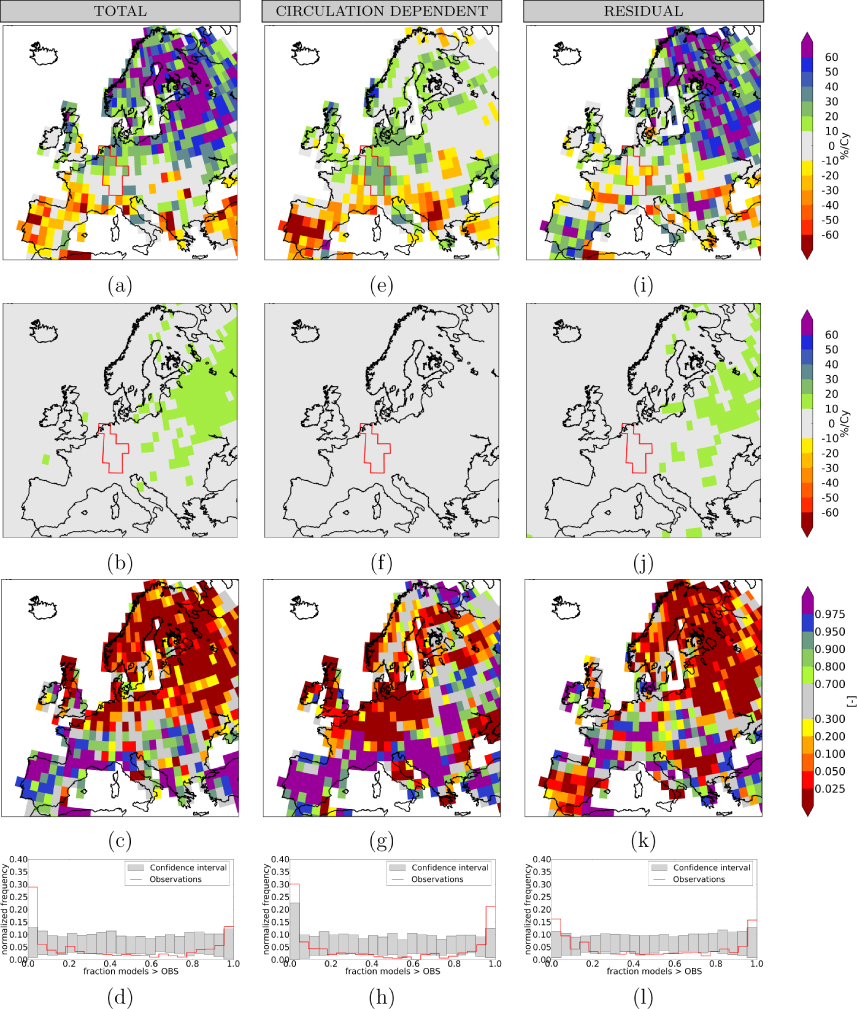
Figure 2. Comparison of observed and GCM RX10day precipitation trends of January–March for 1950–2012. (a) Relative trend in observed precipitation (%/century). (b) Mean relative trend in the CMIP5 ensemble (%/century). (c) Fraction of the CMIP5 ensemble with a trend larger than the observed one (−, non-linear scale). (d) Rank histogram. (e)–(h) Same but for circulation dependent precipitation. (i)–(l) Residuals.
Download figure:
Standard imageThe underestimation of the trend in extreme precipitation could originate from a number of possible causes: (1) the coarse resolution of global climate models may not be enough to describe extreme precipitation events, or may not provide enough detail on local conditions such as topography and coastlines that could affect modeled precipitation; (2) climate models underestimate natural variability of extreme precipitation; (3) underestimation in change of mean circulation characteristics.; (4) model errors (unrelated to atmospheric circulation) present in both GCMs and RCMs; (5) observational errors. We investigate the contribution of points 1–3 to the underestimation of trends in extreme precipitation. The contributions of points 4 and 5 are part of the remaining error budget.
To investigate if the trend bias is caused by the coarse resolution of GCMs we performed the same analysis with a multi-model ensemble of RCMs. We used the ensemble provided by Research Theme 2b of the European ENSEMBLES project, RT2b. The RCM ensemble has, with exception of details, similar trend biases as the ensemble composed of GCMs (not shown).
A second reason for the low reliability of climate models could be an underestimation of natural variability of extreme precipitation in climate models. Year-to-year natural variability is indeed underestimated in GCMs (standard error of the trend estimate for the models is smaller than for the observations), but this is not the case for RCMs (not shown). It is therefore unlikely that the trend bias is caused by an underestimation of natural variability on short time scales in the models. Underestimation of natural variability on multi-decadal or longer time scales could still be possible.
As discussed in section 1, particular circulation types may be more favorable for extreme precipitation events to occur. Using the statistical model defined by equations (1)–(3) we estimate atmospheric circulation induced precipitation changes. The observed/modeled circulation dependent trend, within the linear approximation of equations (1)–(3), is given in figures 2(e) and (f). The residual part of the trend that is not linearly dependent on circulation changes is given in panels (i) and (j).
Seasonal mean circulation changes (figure 3(a), the pattern is consistent over NCEP/NCAR, 20C and Trenberth) cause an increase in observed extreme precipitation in parts of central and northern Europe, as well as a decrease in much of southern Europe. The CMIP5 models also show a north–south dipole in the pressure trends over continental Europe, although on average much weaker and more southeasterly displaced (and a trend to lower pressures over Greenland). Although, this pressure change also causes a (slightly displaced) north–south precipitation response, the response is too weak to show up in figure 2(e). Figure 2(g) (with a summary in 2(h)) shows the fraction of the CMIP5 models with a circulation dependent trend larger than the observed circulation dependent trend. The observed circulation dependent trend caused by a change in geostrophic winds is larger than in any of the models for large parts of northern (increase in precipitation) and southern (decrease in precipitation) Europe. For northern Europe this shows up in an underestimation of the total trend by the models. The circulation dependent decrease in southern Europe is (partly) canceled out by an increase due to other factors. Inconsistencies in the underlying data provides low confidence in the results in the Balkan area. We did not find obvious problems in the Iberian Peninsula so we would have to assume that the (partial) cancelation is real in this area.

Figure 3. Observed (a) and modeled (b) trend in mean JFM sea-level pressure (1950–2012) (hPa/century). (c) Fraction of models with a trend larger than observed (−, non-linear scale).
Download figure:
Standard imageA possible explanation for the residual trend in the far north and in eastern Europe is a strong temperature increase in these regions. When the temperature increases, so does the water-holding capacity of the atmosphere, which in turn favors stronger rainfall events (IPCC 2007). An alternative explanation is that decreasing sea ice extent results in more open water, increasing evaporation.
5. Trend in the Rhine basin
We consider the trend in extreme 10 day precipitation over the Rhine basin (figure 1(a)). These trends are important for flood risk management in the Netherlands.
Figure 4(a) shows the observed and modeled trends in JFM RX10day as averaged over the Rhine basin area. The trend is calculated as the trend of the area average. The observed trend lies on the outer edge of the spread of modeled trends. We verified the results in an ensemble of regional climate models forced by global models (European ENSEMBLES RT2b), producing similar results (not shown).
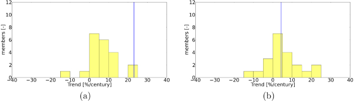
Figure 4. Observed modeled area average JFM RX10day trend for the Rhine basin (1950–2012). Total (a) and residual (b) trend for the Rhine basin. Observed trend is indicated by the blue line, models by the yellow bars.
Download figure:
Standard imageA large part of the trend in this region is, within the linear approximation of a statistical decomposition, caused by a change in circulation (figure 2). In a similar manner as before, we estimate the atmospheric circulation induced precipitation changes for the whole basin, where the averaged change in geostrophic wind anomalies over the basin area is used. We find that a large part of the observed trend is linearly related to changes in mean atmospheric circulation. For the models the effect of circulation is much smaller. Adjusting for the circulation trend mismatch by only considering the residual component, the observed trend is well within the climate model ensemble (figure 4(b)).
6. Conclusions
Climate model based projections of future precipitation extremes are often used in projections of future river discharge extremes. Here, the trends in extreme precipitation in Europe and the Rhine river basin over the last 60 years are compared with observed trends. A correct representation of past changes is an important (but not sufficient) condition to have confidence in projections for the future.
We find that climate models underestimate the trend in extreme precipitation in the northern half of Europe: the trend bias is significant in this area. Using a statistical decomposition we split the trend in a part that is linearly related to circulation change, and a residual part that is not linearly related to circulation change. Circulation changes have caused an increase in observed extreme precipitation in parts of mid and northern Europe, as well as a decrease over the Iberian Peninsula. Climate models underestimate the change in circulation over the past century and as a result have a much smaller (extreme) precipitation response.
Climate models are not capable of reproducing the observed trend in extremes for the Rhine basin. The underestimation is, within the linear approximation of a statistical decomposition and statistical uncertainties, caused by an underestimation of the change in mean circulation. The ensemble covers the observed trend when only the part of the trend not linearly related to mean circulation change is considered: the residual biases not linearly related to mean circulation changes are relatively small. Therefore, it is important that we improve our understanding of circulation changes, in particular related to the cause of the apparent mismatch between observed and modeled circulation trends over the past century (Haarsma et al 2013).
Acknowledgment
The research was supported by the Dutch research program Knowledge for Climate.