

Abstract
The fate of live forest biomass is largely controlled by growth and disturbance processes, both natural and anthropogenic. Thus, biomass monitoring strategies must characterize both the biomass of the forests at a given point in time and the dynamic processes that change it. Here, we describe and test an empirical monitoring system designed to meet those needs. Our system uses a mix of field data, statistical modeling, remotely-sensed time-series imagery, and small-footprint lidar data to build and evaluate maps of forest biomass. It ascribes biomass change to specific change agents, and attempts to capture the impact of uncertainty in methodology. We find that:
• A common image framework for biomass estimation and for change detection allows for consistent comparison of both state and change processes controlling biomass dynamics.
• Regional estimates of total biomass agree well with those from plot data alone.
• The system tracks biomass densities up to 450–500 Mg ha−1 with little bias, but begins underestimating true biomass as densities increase further.
• Scale considerations are important. Estimates at the 30 m grain size are noisy, but agreement at broad scales is good. Further investigation to determine the appropriate scales is underway.
• Uncertainty from methodological choices is evident, but much smaller than uncertainty based on choice of allometric equation used to estimate biomass from tree data.
• In this forest-dominated study area, growth and loss processes largely balance in most years, with loss processes dominated by human removal through harvest. In years with substantial fire activity, however, overall biomass loss greatly outpaces growth.
Taken together, our methods represent a unique combination of elements foundational to an operational landscape-scale forest biomass monitoring program.
Export citation and abstract BibTeX RIS

Original content from this work may be used under the terms of the Creative Commons Attribution 3.0 licence.
Any further distribution of this work must maintain attribution to the author(s) and the title of the work, journal citation and DOI.
1. Introduction
Predicting the fate of carbon in forests under future climates is a fundamental scientific and management challenge, as these systems contain large reservoirs of carbon, provide many essential ecosystem services, and represent a potentially critical feedback in global climate change (Birdsey et al 2007). Yet carbon storage in forested ecosystems can be highly dynamic, affected by diverse anthropogenic and natural disturbance processes that can radically change the carbon trajectory of a landscape (Chambers et al 2007, Environment-Canada 2006, Williams et al 2016). Models and decision support tools that cannot realistically incorporate the full range of disturbance and growth processes can only provide a snapshot of the carbon dynamics, and may not fulfill the needs of the public or of policy makers (Joyce et al 2009). Moreover, neither models nor management plans can exist in an historical vacuum: both must consider how the potential future conditions relate to past and current trends and status (Birdsey 2006).
Our understanding of possible forest carbon futures is hampered by our sparse observations of the recent carbon past. In the United States, the core tool used for national and international reporting of forest carbon fluxes (EPA 2016) has traditionally been the field measurements collected by the Forest Inventory and Analysis (FIA) program (Goodale et al 2002, Woodbury et al 2007). Though FIA measurements are now recorded consistently, cover the contiguous US, and are statistically defensible, the goal of any such inventory program is an estimate of growing stock or volume for large areas (McRoberts et al 2014). This result may not be sufficient for managers and modelers who need spatially explicit maps of carbon and carbon change at the scale of management (Sannier et al 2016). Additionally, the decadal repeat period of FIA plot measurements (in the western US) is longer than that needed to capture anthropogenic and natural processes that significantly alter carbon pools every year (Houghton 2005).
Other tools have the potential to complement FIA plot information in capturing actual forest carbon conditions, but none can fully address carbon dynamics alone. Maps based on small-footprint lidar (light detection and ranging) data have been shown to provide excellent estimates of live aboveground forest biomass and hence carbon (Hudak et al 2002, Kim et al 2009, Naesset 2002, Pflugmacher et al 2014), but these data are generally available for relatively small areas, and even in the future are unlikely to be repeated frequently enough over large areas to capture disturbance processes in a monitoring framework. Maps of forest disturbance from Landsat satellite imagery have fine enough spatial resolution to capture individual patches of disturbance and growth (i.e. 30 × 30 m), and also to meet the criterion of covering large areas (Hansen and Loveland 2012, Huang et al 2010). Landsat-based maps of forest dynamics have traditionally had greatest success focusing on high-severity, abrupt disturbances such as clearcuts and fires (Cohen et al 2002, Masek et al 2013).
While characterizing abrupt disturbance processes is critical for understanding biomass dynamics, maps showing the timing of such disturbance processes alone are insufficient for biomass monitoring. They omit key lower-severity anthropogenic disturbances such as mechanical thinning, subtle or long-lasting natural disturbances caused by insects and drought (Cohen et al 2016, McDowell et al 2015), and slow aggradation processes such as forest growth. Additionally, maps of disturbance timing alone provide no indication of the biomass status before the disturbance, nor of the agent that caused it—both of which can substantially alter the biomass consequences of a given change (Williams et al 2016). Other efforts to map biomass or disturbance at broad spatial extents from satellite-based data (optical, radar, and lidar) have generally focused on single-date estimates of biomass stock (Goetz et al 2009, Kellndorfer et al 2000, Swatantran et al 2011, Zheng et al 2004) or have spatial grains too large to adequately capture change caused by management (Blackard et al 2008, Wilson et al 2013). Uncertainties introduced throughout the modeling process are rarely imparted to users, despite the recognized need for such estimates (Saatchi et al 2011, Sexton et al 2015, Williams et al 2016).
Here, we describe an empirical forest biomass monitoring system that meets many of these challenges. We link FIA plot data with time-series analysis of satellite imagery to create yearly maps of forest biomass at the regional scale, and link changes in those biomass maps to disturbance and growth dynamics. In the process, we examine methodological uncertainties, and utilize high-quality, lidar-based local-scale maps of biomass to understand robustness of our regional estimates. Taken together, the yearly estimates of biomass, biomass uncertainty, and cause of change delivered by our monitoring system can provide a nuanced understanding of the spatial and temporal patterns of forest biomass dynamics at a regional scale.
2. Methods
2.1. Overview
The biomass monitoring system is built from three methodological components (figure 1): (1) regional-scale time-series image analysis using LandTrendr (Kennedy et al 2010, 2015); (2) statistical linkage of that imagery with field plot data using the gradient nearest neighbor (GNN) methodology (Ohmann et al 2012); and (3) local-scale assessment using airborne lidar data (Kane et al 2010).

Figure 1. An observation-based, empirical carbon monitoring system. From left, satellite-data are analyzed through a time-series algorithm (LandTrendr; Kennedy et al 2010) to create disturbance maps, change agent maps, and temporally-stabilized yearly image time-series. Those images are linked via statistical algorithms (GNN: gradient nearest neighbor imputation (Ohmann and Gregory 2002)) with plot data (FIA: forest inventory analysis) and other geospatial data to create yearly maps of plot-like information. That information includes tree-level species and height information, which can be used in allometric equations to create yearly biomass maps at at 30 m grain size. These maps can be used to characterize biomass status in a consistent manner across large or small ownerships, or to examine how change in biomass is affected by anthropogenic or natural agents of change. Where available, these regional-scale biomass maps can be compared to small-area maps of biomass derived from small-footprint lidar acquisitions.
Download figure:
Standard image High-resolution imageMethodological uncertainty is explicitly incorporated into the system. Rather than providing only a single solution for biomass estimation at any given location, we create a suite of scenarios of the biomass landscape for each pixel and year, yielding both the central tendency and an estimate of methodological uncertainty. We then characterize trends in biomass according to the timing and type of agents causing change, including both human and natural processes.
2.2. Study area and datasets
We prototyped our biomass monitoring system in the Western Cascades province of Oregon and a small part of California (see section S1 for details). This study area contains some of the most carbon-rich conifer-dominated forests in the world (Smithwick et al 2002, Waring and Franklin 1979), with a wide range of disturbance and recovery dynamics (Kennedy et al 2012, Moeur et al 2011).
The monitoring system is built from four broad classes of data. Forest inventory data measured in the field by US federal agencies provide the foundational measurements of individual trees at a sample of locations across the study area. Imagery from the Landsat satellites provide the spatial and temporal descriptions of the landscape as it changes over time. Ancillary geospatial data describe the broad environmental conditions, including soil, elevation, and climate. Finally, airborne lidar (laser range-finding) data are used opportunistically to assess performance of the system at focal areas.
2.3. Analysis
2.3.1. Image analysis with LandTrendr
Applying simple statistical tools to spectral data, the LandTrendr algorithms distill the dominant disturbance and recovery processes for each pixel in a Landsat Thematic Mapper time-series (Kennedy et al 2010). LandTrendr image analysis fills two roles. First, it provides stabilized imagery on which the later GNN mapping is based. By removing factors that introduce year-to-year spectral noise, this 'temporally stabilized' imagery allows development of a single, consistent GNN model across time. These stabilized images not only capture the state of the landscape in a given year, but also whether that state is changing from one year to the next or is stable. Second, data derived from LandTrendr can be used to label the agents that cause abrupt and subtle changes, including clearcuts, partial harvests, fires, and insect attack. For both stabilized imagery and change agents, the ultimate analytical products were 30 m resolution raster images for every year from 1990–2012. While the LandTrendr algorithms have been well-described elsewhere (Kennedy et al 2010, Kennedy et al 2012), we highlight in section S2.1 the changes and key steps in processing that apply to the biomass monitoring system, as well as the tools used to evaluate effectiveness.

Figure 2. Estimates of the relationship between aboveground live-tree biomass (CRM allometrics) predicted from the LandTrendr + GNN imputation approach versus that observed at > 6000 plots across the study area. Shown are mean values from GNN Scenarios 1 biomass shows little bias up through 500 Mg ha−1 (see inset), but slowly becomes underpredicted as biomass increases beyond that value (main graph).
Download figure:
Standard image High-resolution image2.3.2. Gradient nearest neighbor imputation
The GNN method links forest inventory plot data with a suite of geospatial predictor variables to produce regional estimates of forest characteristics from which biomass can be calculated. Also described elsewhere (Ohmann and Gregory 2002, Ohmann et al 2012, Ohmann et al 2014), the GNN method uses canonical correspondence analysis (ter Braak 1986) to develop a multivariate gradient space in which spatial predictor datasets (climate, topography, spectral data) and forest inventory plot observations are linked. In section S2.2, we highlight innovations of the method specific to the biomass monitoring system presented in this contribution. At the end of the GNN modeling, each pixel on the landscape is assigned tree measurements from an inventory plot, from which any derivative metrics (including biomass) can be determined and mapped.
2.3.3. Uncertainty scenarios
LandTrendr and GNN are imperfect models affected by the parameters used to constrain them. To capture the uncertainty in these parameter choices, we ran both LandTrendr and GNN under three parameter scenarios each (labeled LT1, 2 and 3 for LandTrendr scenarios, and GNN 1, 2, and 3 for GNN), resulting in a combination of nine 'uncertainty scenario' predictions for each pixel and year. Details of these scenarios are given in sections S2.1.4 and S2.2.4.
Additionally, the translation from tree measurements to biomass through allometric equations is itself uncertain (Duncanson et al 2015). We used two different families of allometric scaling to estimate biomass from tree measurements in each pixel: those based on Jenkins et al (2003) and those using the component ratio method (CRM; (Heath et al 2008)).
2.3.4. Lidar-based mapping
Airborne lidar data provide insight into the three-dimensional structure of forest stands (Lefsky et al 2002), and, when combined with reliable concurrent field measurements, can yield highly reliable estimates of forest biomass at a point in time (Dubayah and Drake 2000). For one of the two lidar acquisitions in our study domain with appropriate field data, we calculated estimates of aboveground forest biomass. For the second site, we utilized an existing forest biomass map. Details of analysis are provided in section S2.3.
3. Results
3.1. Detection and attribution of change
Results of detection and attribution of change are detailed in section S3, and were accomplished at rates consistent with our prior published work (Kennedy et al 2015, Kennedy et al 2012). Confidence in detection and labeling are highest for abrupt, high magnitude events, such as fires and clearcuts, and lower for subtle and long-duration events, such as insect attack or general decline in vigor (sensu (Cohen et al 2016)).

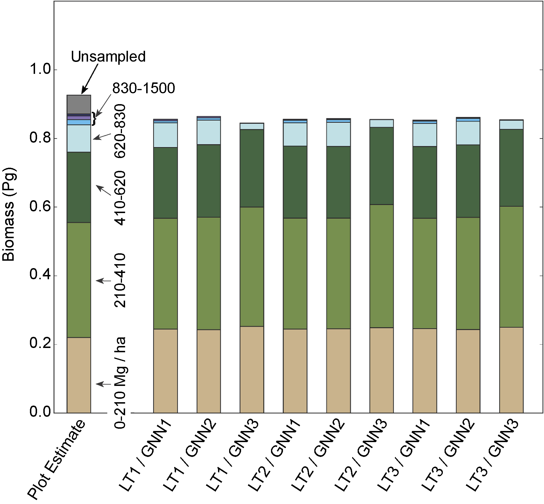
Figure 3. Total aboveground live biomass (using CRM allometry) in the study region, estimated both from plot data expansion factors ('Plot Estimate') and from nine biomass maps derived using the biomass monitoring system described herein. Colors represent the proportion of the total estimated biomass contributed by forests in different biomass densities, shown next to the Plot Estimate bar. Note that all biomass maps underestimate the proportion of biomass in forests above biomass density of 830 Mg ha−1, with GNN 3 scenarios showing the greatest underestimation. Unsampled plots are those not acceesible; they have unknown biomass. As a conservative estimate, we assume they have the same distribution of biomass values as the rest of the measured dataset.
Download figure:
Standard image High-resolution image3.2. Forest biomass estimation with GNN
For the 6108 forest inventory plot measurements in the entire study area, agreement between measured and mean imputed biomass (using GNN scenarios 1 and 2 (section 2.2.4) for all LandTrendr scenarios) was relatively unbiased and 1:1 for biomass densities up to 500 Mg ha−1 (figure 2 inset), and then showed signs of slight underprediction at biomass densities greater than 500 Mg ha−1 (figure 2, main). To understand how these relationships would affect estimates of total biomass for the whole region, we used scaling factors on observed plot values to estimate the proportion of the landscape in different biomass categories, calculated total regional biomass within those categories, and compared the total regional biomass to that derived from the nine variants of our biomass maps grouped in the same biomass categories (figure 3). Mapped total biomass agreed well with estimated biomass from sampled plots, both in terms of totals and in terms of the distribution of biomass across biomass categories, but under-represented the very highest biomass categories (greater than 830 Mg ha−1). Underrepresentation of high biomass conditions was accentuated for GNN Scenario 3 runs. Although it is impossible to know biomass of unsampled plots, the conservative approach of assigning biomass in proportion to all sampled plots suggests that our mapped values underpredict biomass across all scenarios. Regardless of LandTrendr or GNN-scenario, Jenkins-based biomass was ~16% higher than CRM-based biomass (figure 3 vs figure S5), consistent with findings of others (Zhou and Hemstrom 2009). The standard deviation among LandTrendr & GNN scenarios, however, was << 1% of the mean, for either CRM or Jenkins based maps. When reporting the remainder of our results, we report only on the CRM-based estimates, as this is the approach currently employed by FIA to estimate nation-wide biomass stocks.
Imputed maps of aboveground live forest biomass showed spatial patterns consistent with expectations for the managed landscapes of this study area (figure 4). For example, for the CRM-based biomass estimation using LandTrendr scenario 1 (LT1) and GNN scenario 1 (GNN 1) figures 4(a) and (b), old-growth conifer forest shows high live tree biomass (>600 Mg ha−1), while recently-disturbed areas show low biomass (0−50 Mg ha−1). Taking the mean value of biomass from all nine scenarios retains the same landscape-scale pattern (figure 4(c)), but reduces the pixel-scale spatial variability resulting from the nearest-neighbor approach. A map of the variability of biomass across scenarios shows considerable spatial noise (figure 4(d)), but retains some coherent spatial patterns. Generally, variability peaks in the middle of the range of values (figure 4(e)), but for the majority of the study area, variability in estimates is below 25% of the mean values (figure 4(e) inset). Because all LandTrendr and GNN scenarios are methodologically defensible, this suggests that no single scenario could be used to represent the others. Rather, a user should be aware of both a central tendency (such as the mean value, figure 4(c)) and the standard deviation image (figure 4(d)), consistent with Bell et al (2015).

Figure 4. Example biomass products from the monitoring system. (a) Biomass density (Mg biomass ha−1) for a single scenario (LT 1, GNN 1, GRM) of the system for the year 2005. (b) Detail of (a) as indiciated by black box and arrow. (c) Mean biomass density across all nine scenarios for the CRM allometric family for the same year. (d) Standard deviation of the nine scenario estimates. (e) Density plot of uncertainty, as represented by standard deviation of biomass vs. mean biomass for the entire area shown in (a). Although uncertainty exceeded mean biomass in some cases, more than 50% and 75% of the landscape had uncertainty ratios less than 25% and 50% respectively (inset).
Download figure:
Standard image High-resolution image
Figure 5. Tracking change in biomass. (a) Maps of mean per-pixel biomass across all nine LandTrendr and GNN scenario combinations (see table S1 for LandTrendr scenarios; section S2.2.4 for GNN scenarios) for selected years. (b) Trajectory of biomass for the clearcut indicated by the lower polygon in (a). Charted values are mean across pixels within the clearcut patch for each combination of LandTrendr and GNN scenario (L1 = LandTrendr scenario 1, etc.; G1 = GNN scenario 1, etc.). Note the variability in pre-biomass among GNN and LT scenarios, and the variation in post-disturbance regrowth patterns. (c) As with (b), except for the upper polygon, which illustrates regrowth from a clearcut that occured before the observation period. Note that the y-axis scale is changed to highlight regrowth variability among LT and GNN scenarios.
Download figure:
Standard image High-resolution image
Figure 6. Change in biomass caused by specific agents. For each of the nine scenarios, static biomass (based on CRM) in a year was differenced from the prior year, and the mean of all changes summarized at the pixel scale by change agent and summarized across the entire study area. When abrupt disturbances occurred in patches less than ~1 ha, we labeled them as 'unknown abrupt.' Unknown slow changes corresponded with long, slow decline in vegetative signal that could not be ascribed to observable insect or disease outbreaks, but are typically resultant from a mixture of 'decline' factors (Cohen et al 2016).
Download figure:
Standard image High-resolution image3.3. Comparison with lidar-derived estimates
We examined the relationship between biomass estimated from lidar and from LandTrendr + GNN at two forest sites. At the 30 m pixel scale, the relationship was noisy, but it improved with spatial aggregation (section S5, figure S6). For the HJA, the relationship tracked well up until approximately 450 Mg ha−1, and then abruptly plateaued (figure S6), while biomass values remained less than 450 Mg ha−1 at the Deschutes site. Maps of disagreement confirm that discrepancies were greatest in high-biomass stands at the HJ Andrews.
3.4. Change in biomass
By creating yearly biomass maps from 1990–2012, the monitoring system allows comparison at a range of temporal aggregation scales, from the whole period to yearly. At any given point or for any given patch or area, the biomass trajectory over the entire period can be tracked, showing the impacts on biomass of both disturbance and regrowth (figure 5) and how different modeling scenarios affect estimates. Notably, it is unlikely that any single modeling scenario is best under all conditions, as illustrated by the variability in representation of both pre-disturbance condition and post-disturbance recovery rate among scenarios (figures 5(b) and (c)).
For a monitoring system, it is important to document not just how much biomass is changing over time, but why. By linking maps of change agent with maps of mean biomass change, we can ascribe biomass loss and gain to specific agents over time (figure 6). For this study area, we found that anthropogenic changes (clearcuts and partial harvests) were a consistent loss signal over the entire time period, with occasional large loss from fire. Net change recorded by our system switched from general uptake in the 1990s to loss in the 2000s.
Because our system produces multiple estimates of biomass change for each time period, it allows assessment of the uncertainty of the impact of each agent (figure 7). Uncertainty in biomass loss due to clearcuts and partial harvests is low relative to the mean estimated loss, and generally consistent across time (figures 7(a) and (b)). Uncertainty in loss due to fire scales with overall loss rate, which itself is quite variable from year to year (figure 7(c)). Both of these findings emphasize that estimates of biomass immediately after abrupt disturbances can be relatively uncertain, making the estimates of loss span a wider range than the pre-disturbance biomass. Uncertainties associated with long, slow disturbance and with regrowth (figures 7(e) and (f)) were greater than for the other agents, but were relatively consistent over time. Even considering the uncertainty in estimates, loss from long, slow disturbance, which is often associated with pests and other stressors (Cohen et al 2016), exceeds loss from the two insect agents that were explicitly modeled (bark beetle and western spruce budworm, Meigs et al 2015).

Figure 7. Mean biomass loss or gain attributable to individual agents of change (a) clearcuts, (b) partial harvest, (c) fire, (d) known insect, (e) unknown slow disturbance, and (f) recovery. Black line indicates mean change in biomass across all nine LT and GNN scenarios for all cases of a given agent per year, and grey shading shows variability in biomass estimation across the nine modeling scenarios.
Download figure:
Standard image High-resolution image
4. Discussion
Forests occupy an important component of any carbon monitoring program. They have the capacity to store substantial amounts of carbon in live aboveground biomass, but they are also subject to disturbances that remove it. For carbon accounting and risk analysis, a carbon monitoring system must track forest biomass consistently across space and time, and must track how natural and anthropogenic processes change it. Below, we highlight strategies, strengths and weaknesses, and findings of our system. Substantially more detail can be found in supplemental section S6 available at stacks.iop.org/ERL/13/025004/mmedia.
Our monitoring strategy used advanced algorithmic approaches to leverage strengths of complementary datasets. Spectral information from satellite data are ubiquitous and can track change over time, but saturate in high biomass systems. Plot data are the gold standard in biomass estimation, but are sparse in space in time. In our system, temporal segmentation provided the stability of optical data needed to build large plot databases, and the nearest neighbor imputation approach allowed high biomass data to be included in mapped outputs. Although our estimates of biomass show signs of saturation, they did so at relatively high densities (450 or 500 Mg ha−1, figures 2 and 3), suggesting utility in many forested systems. Spatial scale matters, however. At pixel scales, noise vastly swamps signal (figure S6), meaning our system's estimates of absolute biomass at one point in time are not appropriate at the pixel scale; ongoing work explores this scale effect (Bell et al in preparation). However, tracking relative change in biomass over time appears possible even at the scale of individual forest stands (figure 5).
Because our system relied on temporal segmentation of Landsat imagery, it was possible to explicitly tie change in biomass to disturbance and growth changes. While the detection of disturbance from remote sensing contained error (tables S2 and 3), such tight coupling allowed comparison of the carbon impacts of different change agents (figure 6). Importantly, labeling agents of change depended heavily on scaling local knowledge of disturbance through machine learning algorithms.
Our ensemble approach to estimating uncertainty is imperfect and incomplete, but provides a first approximation of the spatial and temporal pattern of the unknown. Not strictly error, our uncertainty maps essentially point to places and times where the system behaved poorly. This can provide insight into where and how the information content or the assumptions of the empirical system break down.
Although our results in a high biomass forest system are encouraging, some caution is needed when considering application of our monitoring system in other forest types. The availability and quality of our core datasets may represent a best-case scenario compared to other areas. Historical Landsat data in the continental US are temporally dense, and the climate of our study region allowed high probability of obtaining cloud-free observations. Similarly, the FIA plot network is unusually robust in quality, design, and temporal depth. These conditions would not be easily met in many tropical systems, for example, where cloud cover and image availability limit spectral information, and access and cost constraints make direct measurement challenging. Additionally, the strength of the relationships between spectral data and forest type data may differ in forest types unlike those tested here, which were dominated by evergreen conifer types. In sparse forests, shrublands, or broadleaf deciduous systems, robustness of prediction would need to be tested explicitly before implementing our system.
Nevertheless, by providing a consistent monitoring framework across which different agents of change can be compared, our system yields several compelling insights in our forest-dominated study area. Human activities control the biomass removal in most years. Fire is sporadic, but when it occurs shifts the system strongly into carbon loss. Note that while our system simply measures removal from the landscape and does not track the fate of that biomass (or carbon), the tight coupling of agent and biomass loss could be used to estimate differential fates of carbon in fires, harvests, and other processes. Interestingly, loss of carbon from known insects was not as great as loss due to other slow degradation processes. The challenge in interpreting this finding is the non-specific nature of those processes: broadly described as 'decline' (Cohen et al 2016), they appear to be real phenomena, but are a mix of other insects, disease, drought effects, and other stressors. Our own estimates show substantial uncertainty in their biomass impacts, leading us to caution against over-interpretation of their importance without further study.
Overall, our system appears viable as another tool for managers and modelers of forest carbon. It provides consistent spatial and temporal estimates of forest biomass dynamics, and attempts transparent inclusion of errors and uncertainties. By linking agents of change with biomass change, it provides tools to managers and modelers to understand impacts and evaluate possible alternative future scenarios.
5. Conclusion
We have presented an empirical approach to monitoring live forest carbon at broad scales, using a mix of field data, statistical modeling, remotely-sensed time-series imagery, and small-footprint lidar data. The framework builds maps of forest biomass state for each year that are consistent and comparable across years, and is constructed to allow direct coupling of change in biomass to specific change agents. Several important findings emerge from this work:
- 1.A common image framework for biomass estimation and for change detection allows for consistent comparison of both state and change processes controlling carbon dynamics.
- 2.Although biomass estimation with optical sensors tends to saturate using traditional statistical methods, the nearest-neighbor imputation approach allows us to better capture the full range of values (including very high biomass) at the ecoregion scale.
- 3.Comparison with estimates from lidar data shows general agreement, but also shows local-scale disagreement at the scale of pixels and forest stands. This suggests that there is a lower limit on the spatial detail at which this regional scale method can be applied. Further investigation to determine the appropriate scales is underway.
- 4.Variability in controlling parameters for both the time-series fitting and the imputation approach do result in variability in biomass estimates at the pixel scale, but using the mean of these ensembles improves the overall fit between observed and predicted values. Importantly, the variability in biomass estimates caused by methodological differences is markedly less than the different in biomass estimates caused by use of different allometric scaling equations.
- 5.In this forest-dominated study area, growth and loss processes largely balance in most years, with loss processes dominated by human removal through harvest. In years with substantial fire activity, however, overall biomass loss greatly outpaces growth.
Acknowledgments
This work was funded through USDA NIFA Grant 2011-67003-20458 and NASA Carbon Monitoring System Grant NNX12AP76G.