

Abstract
To explore whether the large-scale patterns of biomass allocation vary by climate, soil, and forest characteristics in terrestrial ecosystems, on the basis of the national forest inventory data (2004–2008) and our previous field measurements (2011–2012), we investigated the variation of four biomass allocation fractions (BAFs), and their relationship with environmental factors (e.g. climate and soil chemistry) and forest characteristics (e.g. stand age and stand density) across 11 of China's forest types. Our results revealed that BAFs have significant latitudinal, longitudinal and altitudinal trends. Stepwise multiple regression models that involve the climate, soil and forest stand properties account for a part of the biogeographical variation in BAFs, and the stand age, stand density and mean growing season temperature mainly explain these variations. Reduced major axis regression models showed that BAFs differ in their sensitivity (slope of their response to environmental gradients) to climate, soil and forest characteristics among different forest types. The results of the current study do not support the isometric allocation hypothesis, which suggests that component biomass scales equivalently as total biomass across different plant species along environmental gradients.
Export citation and abstract BibTeX RIS

Content from this work may be used under the terms of the Creative Commons Attribution 3.0 licence. Any further distribution of this work must maintain attribution to the author(s) and the title of the work, journal citation and DOI.
1. Introduction
Forests cover about 30% of the land surface of the Earth and 283 Gt carbons (C) are stored in global forest biomass; therefore, they play an important role in global C cycling (Dixon et al 1994, Houghton et al 2000, Piao et al 2003). When new biomass (net primary production) produces via photosynthesis, the proportional allocation of new biomass to leaves, branches, stems and roots results in the proportional distribution of standing biomass C among these biomass components (Reich et al 2014). Such processes can be influenced by plant age, resource supply, and/or climate (Poorter et al 2009, 2012, Hui et al 2012). The general lack of knowledge about biomass allocation is critical to the accuracy of global C cycle modeling and accounting (Fan et al 1998, Brown et al 1999).
Root/shoot ratios (R/S) have been used to calibrate and estimate C storage from easily measurable aboveground biomass, and have also been incorporated into terrestrial ecosystem C modeling (Sack et al 2002, Scurlock et al 2002, Milchunas 2009). Compared with R/S, biomass allocation fractions (BAFs, defined as the ratios of plant biomass components (stems, branches, foliage, and roots) and total plant biomass), are biologically clear, and are well grounded in plant growth theory (Körner 1994, Poorter et al 2009). The use of BAFs retains the maximum amount of information because all ratios can be calculated from BAFs (Poorter et al 2012), and it might be useful to separate the plant bodies of larger woody species into even more categories (Körner 1994, Poorter et al 2012). Moreover, why the biomass allocation patterns vary along environmental gradients were continuously debated in theoretical ecology (Cheng and Niklas 2007, McCarthy & Enquist 2007, Poorter et al 2012). The isometric hypothesis suggests that the component biomass scales isometrically with total biomass across a diverse range of different plant species (Euquist and Niklas 2002, Niklas 2005) and community types (Cheng and Niklas 2007). In contrast, the optimal partitioning hypothesis suggests that plants respond to variations in environmental conditions by allocating biomass among different organs to capture nutrients, water, and light to maximize their growth rate (Bloom et al 1985, Chapin et al 1989). According to this hypothesis, plants allocate proportionally more biomass to leaves in high-nutrient (or moisture) environments, and shift more biomass to roots in low-nutrient (or moisture) conditions (Müller et al 2000). Large-scale observations of biomass in various vascular plants have supported the existence of isometric allocation (Euquist and Niklas 2002, Niklas 2005). However, the results of some manipulative experiments contradict this hypothesis (e.g. Shipley and Meziane 2002, McCarthy and Enquist 2007). This inconsistency might be due to lack of consideration of the interactions between plants and environmental factors (Li et al 2005, Hui et al 2012). A meta-analysis also indicated that the patterns of biomass allocation to leaves, stems, and roots in vegetative plants were influenced by the growth environment or growing condition, plant size, evolutionary history, and competition (Poorter et al 2012). Although the studies mentioned above had summarized the influence of growth environment, plant size, evolutionary history and competition on biomass allocation patterns to leaves, stems and roots in vegetative plants, however, the knowledge of BAFs in relation to biogeography and environmental effects is still unclear.
China offers a unique opportunity for examining the relationship between BAFs and environmental factors across different terrestrial ecosystems in large scale because it contains complex forest characteristics (e.g. age, density, and forest types) and soil nutrients under various climatic conditions (e.g. temperature and precipitation) (Zhao and Zhou 2006). In addition, biotic and abiotic factors such as climate, soil conditions, and forest age are believed to account for a large amount of forest C stocks (Brown 2002). Therefore, a better understanding of their relative contributions to forest carbon storage is fundamentally important to make environmental policies and manage ecosystem C to enhance the forest C sink. However, despite the progress made to date, the large-scale pattern of the biomass allocation fractions (BAFs) in China's forest remains poorly defined.
In this study, we investigated the BAFs of forest leaves (LMF), branches (BMF), stems (SMF), and roots (RMF) by using a large-scale biomass survey across the forest communities in China. Our objectives were as follows: (1) to document the biogeographical patterns of BAFs in plants at a national scale, (2) to examine the sensitivity of BAFs to forest characteristics (e.g. age, density, and forest types) and soil nutrients and climatic factors (e.g. temperature and precipitation), and (3) to explore whether component biomass scales isometrically with total biomass across different forest types at the community level.
2. Material and methods
2.1. Large-scale forest biomass data
The forest biomass, stand age and density at 1022 sites across China (figure 1) were obtained from national forest inventory data at 912 sites during from 2004 to 2008 (Luo et al 2012) and our field survey data for forest carbon at 110 random sites across southern China from 2011 to 2012 (Zhang et al 2014). For each site in our fields, three 20 × 50 m replication plots were first established in one sampling site for all field surveys. Then, each plot was divided into ten 10 × 10 m quadrats. Height and tree diameter at breast height (DBH) of each individual tree for stems with DBH ≥ 2 cm and the total number of individuals in each plot were recorded. Based on the height and DBH measured above, five to seven live trees with no defect of different diameter class sizes for each species within a plot were randomly selected for cutting and weighing of their component parts (stems, branches, leaves, coarse root and fine root). Representative samples of the stems, branches, leaves and roots of standard trees were then taken back to the laboratory, dried, and used for calculation of the relationship between dry and fresh weights. Leaf ( branch (
 stem (
 and root biomass (
 per hectare in each site were then computed by biomass components of all trees, respectively, and total biomass (
 in each site was the sum of

 and
and  The ages of selected trees were measured by counting tree-rings using the TSAP-Win computer program (F.Rinn Engineering Office and Distribution, Heidelberg).

Figure 1. Locations of the 1022 sampling sites across the major forest types in China.
Download figure:
Standard image High-resolution imageNational forest inventory data were also complied and tree biomass components (stems, branches, leaves, and roots) for stems with DBH ≥ 2 cm in each site were estimated with the method described as above (Luo et al 2012). A total of 1022 average values of all tree components (leaves, branches, stems, roots, and total plants) per hectare in each site were included in the dataset. Site-related information, site conditions (longitude, latitude, altitude), forest characteristics (stand age, stand density, and forest type), soil chemistry (pH, total nitrogen (TN), and total phosphorus (TP), and climate factors (e.g. mean annual temperature (MAT), mean annual precipitation (MAP), growing season temperature (GST), growing season precipitation (GSP), potential evapotranspiration (PET, mm), and aridity index (AI, PET/MAP)) were also documented in the dataset (see appendix data S1 and table 1 for details).
Table 1. Site conditions (longitude, latitude, altitude), forest characteristics (stand age, stand density), soil chemistry (pH, total nitrogen (TN), and total phosphorus (TP), and climate factors (e.g., mean annual temperature (MAT), mean annual precipitation (MAP), growing season temperature (GST), growing season precipitation (GSP), potential evapotranspiration (PET, mm), and aridity index (AI, PET/MAP)) across different forest types in China.
| Forest types | BTLF | BAPF | TPTF | TSPF | SPPF | SPMF | SMPF | SCLF | SEBF | TRMF | DRW |
|---|---|---|---|---|---|---|---|---|---|---|---|
| Longitude (°) | 86.4–131.8 | 81.1–131.8 | 103.8–129.5 | 85.2–134.0 | 97.4–104.9 | 105.1–120.6 | 85.2–119.3 | 103.4–121.6 | 85.2–120.1 | 104.7–117.9 | 80.6–88.1 |
| Latitude (°) | 28.6–52.6 | 26.1–52.6 | 32.6–42.6 | 25.8–52.5 | 24.7–28.6 | 21.8–32.7 | 24.9–36.4 | 18.7–32.3 | 20.7–30.3 | 18.6–24.4 | 38.4–48.0 |
| Altitude (m) | 441–4240 | 410–4200 | 240–3200 | 150–3640 | 206–3300 | 110–1420 | 10–3558 | 20–1910 | 80–4160 | 10–875 | 500–950 |
| Stand age (years) | 30–195 | 46–350 | 15–95 | 25–222 | 20–150 | 15–101 | 16–160 | 16–55 | 3–200 | 18–110 | 25–53 |
| Stand density (no./ha) | 219–9535 | 125–3967 | 146–8506 | 149–7320 | 89–7239 | 392–3600 | 183–6195 | 1018–4978 | 150–9057 | 300–208 00 | 100–2406 |
| Soil pH | 4.2–8.7 | 4.6–8.7 | 4.6–7.5 | 5.0–8.8 | 4.8–6.2 | 4.9–6.2 | 4.8–6.2 | 4.8–6.5 | 4.8–6.9 | 4.7–6.9 | 7.5–8.3 |
| Soil TN (g kg−1) | 0.1–25.8 | 0.2–2.6 | 0.4–1.6 | 0.4–2.5 | 1.9–2.6 | 0.4–1.6 | 0.4–2.4 | 0.4–1.6 | 0.4–2.6 | 0.5–1.5 | 0.1–0.4 |
| Soil TP (g kg−1) | 0.2–15.9 | 0.2–1.6 | 0.2–0.7 | 0.2–1.6 | 0.6–1.6 | 0.2–0.7 | 0.2–0.7 | 0.2–0.7 | 0.2–1.6 | 0.2–0.7 | 0.2–0.7 |
| MAT (°C) | −6.2–4.2 | −6.6–13.9 | 2.9–13.1 | −5.5–16.0 | 7.5–21.1 | 12.2–24.0 | 5.7–17.0 | 9.4–22.4 | 3.5–24.2 | 2.3–25.2 | 4.6–13.7 |
| MAP (°C) | 371–1274 | 369–1937 | 403–1173 | 241–1283 | 739–1654 | 1023–2006 | 370–2205 | 870–2989 | 636–2323 | 1543–2366 | 27.6–97.2 |
| GST (°C) | 7.3–24.9 | 7.4–26.4 | 7.3–20.4 | 12.3–20.3 | 11.9–19.2 | 13.2–18.8 | 8.3–18.1 | 9.4–18.2 | 6.4–27.1 | 14.0–18.6 | 7.3–15.6 |
| GSP (°C) | 223–2098 | 39–2099 | 84–1596 | 363–1232 | 402–1009 | 497–660 | 370–2205 | 255–890 | 860–1900 | 851–1631 | 110–284 |
| PET (mm) | 576–1358 | 570–1249 | 101–1230 | 606–1125 | 947–1303 | 795–1130 | 504–936 | 679–1064 | 386–1132 | 1031–1161 | 1028–1490 |
| AI | 0.3–8.41 | 0.4–12.1 | 0.2–11.9 | 0.7–2.4 | 1.1–2.6 | 1.3–2.0 | 0.4–2.3 | 1.0–3.6 | 0.3–2.6 | 0.7–1.3 | 4.3–10.6 |
Note: BTLF Boreal/temperate Larix forest, BAPF boreal/alpine Picea abies forest, TPTF temperate Pinus tabulaeformis forest, TSPF temperate/subtropical montane Populus-Betula deciduous forest, SPPF subtropical montane Pinus yunnanensis and P. khasya forest, SPMF subtropical Pinus massoniana forest, SMPF subtropical montane Pinus armandii, P. taiwanensis and P. densada forest, SCLF subtropical Cunninghamia lanceolata forest, SEBF subtropical evergreen broadleaved forest, TRMF tropical rainforest and monsoon forest, DRW desert riverside woodland.
2.2. Climatic variables, soil data, and forest types
Growing season temperature and precipitation are important factors that affect the large-scale pattern of grass biomass allocation (Yang et al 2010). In the current study, we selected GST, GSP, PET (calculated using the Penman–Monteith method), and AI as climate variables. GST, GSP, PET, AI latitude, longitude, and altitude were recorded at each site, and the data were used in the analyses. For records that lacked detailed altitude data, we used three-dimensional topographical maps to acquire this information based on latitude/longitude coordinates. For sites where climate variables were not recorded, the relevant data were estimated with records of 680 climatic stations in China using a Kriging extrapolation method (Luo et al 2012).
Data regarding soil pH, total nitrogen (TN), and total phosphorus (TP) were obtained from the national second soil survey and our field measurements (Han et al 2011). Forests in the dataset included all the major forest types in China, and were grouped into eleven forest types as follows: boreal/temperate Larix forest (BTLF), boreal/alpine Picea abies forest (BAPF), temperate Pinus tabulaeformis forest (TPTF), temperate/subtropical montane Populus–Betula deciduous forest (TSPF), subtropical montane Pinus yunnanensis and P. khasya forest (SPPF), subtropical Pinus massoniana forest (SPMF), subtropical montane Pinus armandii, P. taiwanensis, and P. densada forest (SMPF), subtropical Cunninghamia lanceolata forest (SCLF), subtropical evergreen broadleaved forest (SEBF), tropical rainforest and monsoon forest (TRMF), and desert riverside woodland (DRW) (Li et al 2005).
2.3. Statistical analysis
All data analyses were performed using statistical software SPSS 19.0 (SPSS Inc., Chicago, IL, USA, 2004). BAFs of leaves (LMF), branches (BMF), stems (SMF), and roots (RMF) were calculated as  /
/
 /
/
 /
/ and
and  /
/ respectively (Poorter et al 2012). Analysis of variance (ANOVA) was used to compare the BAFs from different forest types to determine the effect of forest types (species composition) on the geographical patterns of biomass allocation.
Stepwise multiple regression (SMR) was used to identify the effects of climate (e.g. GST, GSP, PET, and AI), soil chemistry (e.g. pH, TN and TP) and forest characteristics (e.g. stand age and stand density) on BAFs. To demonstrate the relative effects of climate, soil and forest characteristics, partial general linear model (GLM) analyses were used to separate the variance explained by different factors into the independent effects of each individual factor and interaction effects between factors (Heikkinen et al 2005). In addition, because the reduced major axis (RMA) regression slopes of the relationship between BAFs and these variations can be used to indicate the response of biomass allocation to variation in climate, soil chemistry and forest characteristics (Sokal and Rohlf 1995), we calculated these slopes for all of the four BAFs for the 11 forest types to analyze the sensitivities of the variations in forest BAFs among forest types. Positive RMA slopes at the forest-type level indicated an increase in BAFs with increasing temperature, precipitation, soil elements etc, and vice versa. To eliminate effects of the different units of these variables on the slope values, each variable was converted to relative values (observation value/mean value) and the RMA slopes were transformed using formula 1, where slopeRMAm is the un-transformed RMA slope of BAF m against all selected variables by the SMR method (Han et al 2011).
3. Results
3.1. Statistical and biogeographic patterns of forest biomass allocation
The BAFs all varied largely across the sites, ranging from 0.74 to 20.03% for LMF, 2.04–40.70% for BMF, 23.96–86.87% for SMF, and 3.18–44.76% for RMF (figure 2). The mean values were 5.80%, 14.73%, 59.84% and 19.63% for LMF, BMF, SMF and RMF, respectively. BAFs also varied markedly across different forest types (table 2). For LMF, the mean ranged from 1.93% (DRW) to 8.87% (TPTF), whereas BMF varied from 8.23% (BTLF) to 19.45% (SMPF). For RMF, the mean value ranged from 10.31% (SPPF) to 26.16% (TSPF). In contrast, the mean SMF was less variable, and ranged only from 50.29% (TRMF) to 69.31% (SPPF).

Figure 2. Frequency distributions of (a) LMF, (b) BMF, (c) SMF, and (d) RMF across forests in China. The mean and median values are presented. LMF, leaf mass fraction; BMF, branch mass fraction; SMF, stem mass fraction; RMF, root mass fraction.
Download figure:
Standard image High-resolution imageTable 2. Biomass allocation fractions (BAFs) across different forest types in China.
| Forest types | LMF | BMF | SMF | RMF | Data number |
|---|---|---|---|---|---|
| BTLF | 3.15 ± 0.08fg | 8.23 ± 0.21d | 65.03 ± 1.32b | 23.59 ± 1.34b | n = 46 |
| BAPF | 4.74 ± 0.17def | 8.45 ± 0.26d | 69.19 ± 0.60a | 17.62 ± 0.29d | n = 167 |
| TPTF | 8.87 ± 0.19a | 13.15 ± 0.22c | 57.97 ± 0.35c | 20.01 ± 0.21c | n = 154 |
| TSPF | 3.89 ± 0.11fg | 13.52 ± 0.35c | 56.43 ± 0.28cd | 26.16 ± 0.36a | n = 125 |
| SPPF | 5.90 ± 0.12cd | 14.47 ± 0.18c | 69.31 ± 0.70a | 10.31 ± 0.55e | n = 54 |
| SPMF | 6.00 ± 0.20c | 14.90 ± 0.65c | 64.14 ± 0.89b | 14.95 ± 0.55de | n = 65 |
| SMPF | 7.81 ± 0.43ab | 19.45 ± 0.98a | 56.87 ± 1.29cd | 15.87 ± 0.59d | n = 57 |
| SCLF | 8.78 ± 0.39a | 9.49 ± 0.29d | 63.15 ± 0.79b | 18.59 ± 0.31cd | n = 98 |
| SEBF | 4.28 ± 0.06ef | 18.93 ± 0.29ab | 58.12 ± 0.32c | 18.79 ± 0.29cd | n = 232 |
| TRMF | 5.24 ± 0.81cde | 19.25 ± 2.20a | 50.29 ± 3.33d | 25.21 ± 2.62a | n = 15 |
| DRW | 1.93 ± 0.30g | 17.59 ± 1.70ab | 64.22 ± 3.27b | 17.36 ± 2.33d | n = 9 |
Note: (1) Values are presented as means ± SE. (2) LMF leaf mass fraction, BMF branch mass fraction, SMF stem mass fraction, RMF root mass fraction; (3) BTLF Boreal/temperate Larix forest, BAPF boreal/alpine Picea abies forest, TPTF temperate Pinus tabulaeformis forest, TSPF temperate/subtropical montane Populus-Betula deciduous forest, SPPF subtropical montane Pinus yunnanensis and P. khasya forest; SPMF subtropical Pinus massoniana forest, SMPF subtropical montane Pinus armandii, P. taiwanensis and P. densada forest, SCLF subtropical Cunninghamia lanceolata forest, SEBF subtropical evergreen broadleaved forest, TRMF tropical rainforest and monsoon forest, DRW desert riverside woodland.
Except for BMF, other BAFs exhibited significant longitudinal trends (P < 0.01; table 3). LMF and RMF increased from west to east, whereas SMF increased from east to west. When latitudinal patterns were analyzed, BMF and RMF decreased and increased from south to north, respectively. In addition, LMF and BMF decreased significantly with increasing altitude, while SMF increased significantly with increasing altitude.
Table 3. Pearson correlations between four biomass allocation fractions (BAFs) and site conditions.
| Site conditions | LMF | BMF | SMF | RMF |
|---|---|---|---|---|
| Longitude (E, °C) | 0.126** | 0.036 | −0.129** | 0.185** |
| Latitude (N, °C) | −0.012 | −0.279** | −0.085 | 0.371** |
| Altitude (m) | −0.149** | −0.222** | 0.251** | −0.030 |
Note: (1) LMF leaf mass fraction, BMF branch mass fraction, SMF stem mass fraction, RMF root mass fraction; (2) * and ** present p < 0.05 and p < 0.01, respectively.
3.2. Relationship between BAFs and climatic, soil and forest characteristics
Stepwise multiple regression (SMR) analysis showed that LMF and RMF were significantly and negatively correlated with GSP and GST (table 4), respectively. SMF were significantly and positively correlated with GST, and BMF were significantly and positively correlated with both of GSP and GST (table 4). The four BAFs also exhibited different sensitivities to climate gradients (table 4). SMF and RMF responded to GST with steeper regression slopes than did GSP.
Table 4. Stepwise multiple regressions (SMR) between four biomass allocation fractions (BAFs) with stand characteristics and environmental factors in China's forests.
| BAFs | Models | Equations | P. | R2 |
|---|---|---|---|---|
| LMF | 1 | LMF = −0.02AGE + 7.04 | 0.001 | 0.096 |
| 2 | LMF = −0.02AGE–0.09TN + 7.12 | 0.000 | 0.124 | |
| 3 | LMF = −0.02AGE-0.01TN-0.001GSP + 7.69 | 0.000 | 0.148 | |
| 4 | LMF = −0.02AGE-0.12TN-0.001GSP-0.25 pH + 9.55 | 0.001 | 0.152 | |
| BMF | 1 | BMF = 0.31GST + 10.92 | 0.000 | 0.116 |
| 2 | BMF = 0.22GST-0.03AGE + 13.72 | 0.000 | 0.161 | |
| 3 | BMF = 0.12GST-0.03AGE + 0.002GSP + 13.03 | 0.000 | 0.177 | |
| SMF | 1 | SMF = 0.08AGE + 56.04 | 0.000 | 0.170 |
| 2 | SMF = 0.08AGE + 0.18GST + 53.62 | 0.003 | 0.186 | |
| 3 | SMF = 0.09AGE + 0.17GST-0.001DENSITY + 54.551 | 0.000 | 0.191 | |
| 4 | SMF = 0.08AGE + 0.20GST-0.001DENSITY + 0.20TN + 54.15 | 0.002 | 0.195 | |
| RMF | 1 | SMF = −0.24GST + 21.65 | 0.000 | 0.086 |
| 2 | SMF = −0.26GST + 0.001DENSITY + 20.62 | 0.000 | 0.143 | |
| 3 | SMF = −0.33GST + 0.001DENSITY-0.02AGE + 23.03 | 0.000 | 0.172 | |
| 4 | SMF = −0.29GST + 0.001DENSITY-0.02AGE + 0.61 pH + 18.83 | 0.002 | 0.181 | |
| 5 | SMF = −0.28GST + 0.001DENSITY-0.02AGE + 0.72 pH + 0.26TP + 17.82 | 0.003 | 0.184 |
Note: AGE stand age, DENSITY stand density, GST mean growing season temperature, GSP mean growing season precipitation, pH soil pH, TN total nitrogen (g/kg) in soil, TP total phosphorus (g/kg) in soil.
LMF significantly decreased with soil pH, soil TN, and stand age, and BMF significantly decreased with stand age (table 4). SMF significantly increased with soil TN and stand age, but decreased significantly with stand density due to lot of competition and less lateral growth (table 4). RMF significantly decreased with stand age, but increased significantly with soil pH, soil TP and stand density (table 4). In addition, SMF responded to stand age with steeper regression slope than did other BAFs, and RMF responded to soil pH with steeper regression slope than did LMF and SMF.
3.3. Sensitivities of the variations in forest BAFs among forest types
SMR indicated that LMFs in BTLF, SEBF and TRMF were significantly and negatively correlated with GST, soil TP and soil pH, respectively, while that in SPPF was significantly and positively correlated with GSP (table 5). Both LMFs in TPTF and SMPF decreased with increasing stand age, and these in TPTF and SMPF decreased and increased with increasing soil TP and soil TN, respectively. LMF in TSPF was significantly and positively correlated with stand density and GSP (table 5). LMF in BAPF was significantly and positively correlated with stand density, while negatively correlated with GST, stand age, soil pH and soil TN. Likewise to LMF, the other three BAFs in the 11 forest types were also affected by different variations of climate, soil chemistry and forest characteristics (table 5).
Table 5. Stepwise multiple regressions (SMR) between four biomass allocation fractions (BAFs) with stand characteristics and environmental factors across different forest types.
| BAFs | Forest types | Equations | P. | R2 |
|---|---|---|---|---|
| LMF | BTLF | LMF = −0.075GST + 3.04 | 0.006 | 0.152 |
| BAPF | LMF = 0.002DENSITY-0.15GST-0.01AGE-1.05TN-0.44 pH + 10.63 | 0.000 | 0.618 | |
| TPTF | LMF = −0.06AGE-0.005GSP + 15.07 | 0.000 | 0.137 | |
| TSPF | LMF = 0.001DENSITY + 0.001GSP + 2.70 | 0.005 | 0.172 | |
| SPPF | LMF = 0.01GSP-1.05 | 0.000 | 0.291 | |
| SPMF | — | — | — | |
| SMPF | LMF = −0.06AGE + 2.46TN + 7.22 | 0.000 | 0.337 | |
| SCLF | LMF = −0.003GSP + 0.13AGE-2.06 pH + 2.37TN + 18.80 | 0.001 | 0.191 | |
| SEBF | LMF = −0.69TP + 4.84 | 0.007 | 0.072 | |
| TRMF | LMF = −0.24 pH + 4.36 | 0.010 | 0.092 | |
| DRW | — | — | — | |
| BMF | BTLF | BMF = −0.001DENSITY + 8.66 | 0.002 | 0.191 |
| BAPF | BMF = 0.001DENSITY-0.33GST-0.02AGE + 11.36 | 0.000 | 0.409 | |
| TPTF | BMF = 0.01GSP + 6.44 | 0.000 | 0.162 | |
| TSPF | — | — | — | |
| SPPF | BMF = 12.98TP + 0.01GSP-0.001DENSITY-5.21 | 0.000 | 0.443 | |
| SPMF | BMF = 0.15AGE + 9.77 | 0.000 | 0.146 | |
| SMPF | BMF = −0.12AGE + 0.005GSP + 18.40 | 0.000 | 0.418 | |
| SCLF | BMF = 0.29GST-1.50 pH + 12.88 | 0.004 | 0.106 | |
| SEBF | — | — | — | |
| TRMF | — | — | — | |
| DRW | — | — | — | |
| SMF | BTLF | SMF = −0.001DENSITY + 1.32GST + 69.92 | 0.000 | 0.563 |
| BAPF | SMF = 0.81GST + 0.04AGE + 1.29 pH-0.003DENSITY + 54.39 | 0.000 | 0.371 | |
| TPTF | SMF = 0.14AGE-0.83GST + 0.01GSP + 48.16 | 0.000 | 0.292 | |
| TSPF | SMF = −1.33 pH-0.001DENSITY + 65.94 | 0.001 | 0.150 | |
| SPPF | SMF = −18.90TP-1.19GST + 93.32 | 0.000 | 0.421 | |
| SPMF | SMF = −0.15AGE + 68.61 | 0.002 | 0.108 | |
| SMPF | SMF = 0.17AGE-0.007GSP + 57.39 | 0.000 | 0.412 | |
| SCLF | SMF = 4.55 pH + 37.99 | 0.022 | 0.094 | |
| SEBF | SMF = −3.71TP-0.001DENSITY + 61.79 | 0.004 | 0.072 | |
| TRMF | — | — | — | |
| DRW | — | — | — | |
| RMF | BTLF | RMF = 0.001DENSITY-1.28GST + 18.43 | 0.000 | 0.609 |
| BAPF | RMF = −0.78 pH-0.002GSP-0.32GST + 1.35TN + 23.29 | 0.000 | 0.264 | |
| TPTF | RMF = −0.02GSP-0.08AGE + 0.45GST + 1.18 pH + 0.94TN + 20.72 | 0.000 | 0.423 | |
| TSPF | RMF = 1.14 pH-3.40TP + 20.30 | 0.009 | 0.173 | |
| SPPF | RMF = −0.43AGE + 11.83 | 0.000 | 0.201 | |
| SPMF | — | — | — | |
| SMPF | RMF = −0.04AGE + 18.47 | 0.000 | 0.106 | |
| SCLF | — | — | — | |
| SEBF | RMF = 5.10TP + 0.001DENSITY + 14.10 | 0.000 | 0.122 | |
| TRMF | RMF = 1.66 pH + 15.22 | 0.006 | 0.091 | |
| DRW | — | — | — |
Note: (1) LMF leaf mass fraction, BMF branch mass fraction, SMF stem mass fraction, RMF root mass fraction; (2) BTLF Boreal/temperate Larix forest, BAPF boreal/alpine Picea abies forest, TPTF temperate Pinus tabulaeformis forest, TSPF temperate/subtropical montane Populus-Betula deciduous forest, SPPF subtropical montane Pinus yunnanensis and P. khasya forest; SPMF subtropical Pinus massoniana forest, SMPF subtropical montane Pinus armandii, P. taiwanensis and P. densada forest, SCLF subtropical Cunninghamia lanceolata forest, SEBF subtropical evergreen broadleaved forest, TRMF tropical rainforest and monsoon forest, DRW desert riverside woodland; (3) AGE stand age, DENSITY stand density, GST mean growing season temperature, GSP mean growing season precipitation, pH soil pH, TN total nitrogen (g/kg) in soil, TP total phosphorus (g/kg) in soil; (4) '—' denotes no proper fitting model.
The RMA analyses revealed that BAFs exhibited different sensitivities to climate gradients across forest types (figure 3). The sensitivity of LMF (assessed using the RMA regression slope) to GST in BTLF was the highest of all forest types. BMF in SMPF and SCLF displayed steeper slopes against the GST than those in other forest types. SMF in SPPF showed more sensitivity to GST than those in other forest types (figure 3). Similarly, LMF in TSPF, SPPF, and SCLF displayed steeper slopes against the GSP than those in other forest types. RMF in BAPF had more sensitivity to GSP than those in other forest types (figure 3). Broadly, BAFs in BTLF, BAPF, TPTF, SPPF, SMPF and SCLF showed more sensitivity to climate than those in other forest types.

Figure 3. Reduced major axis (RMA) regression slopes for four biomass allocation fractions (BAFs; LMF, BMF, SMF, and RMF) against climate, site conditions, soil chemistry, and stand characteristics across eleven forest types in China. RMA slopes for the eight variables (MAT, MAP, soil pH, soil TN, soil TP, altitude, stand age, and stand density) were transformed to eliminate the effects of different units (see Methods). The segmental lengths of the bars directly represent the slopes of the regression lines between BAFs and the total variables. LMF, leaf mass fraction; BMF, branch mass fraction; SMF, stem mass fraction; RMF, root mass fraction; BTLF, Boreal/temperate Larix forest; BAPF, boreal/alpine Picea abies forest; TPTF, temperate Pinus tabulaeformis forest; TSPF, temperate/subtropical montane Populus-Betula deciduous forest; SPPF, subtropical montane Pinus yunnanensis and P. khasya forest; SPMF, subtropical Pinus massoniana forest; SMPF, subtropical montane Pinus armandii, P. taiwanensis and P. densada forest; SCLF, subtropical Cunninghamia lanceolata forest; SEBF, subtropical evergreen broadleaved forest; TRMF, tropical rainforest and monsoon forest.
Download figure:
Standard image High-resolution imageBAFs had different sensitivities to soil chemistry among the different forest types (figure 3). BAFs in BAPF, TPTF, TSPF, SMPF, SCLF and TRMF showed more sensitivity to soil pH than those in the other forest types (figure 3). Likewise, BAFs in BTLF, SPMF and TRMF displayed shallower slopes against the soil TN or soil TP than those in the other forest types. In addition, BAFs in BAPF, TPTF, SPPF and SPMF had more sensitivity to stand age than those in other forest types (figure 3). BAFs in BTLF, BAPF, TSPF, SMPF, SPPF and SEBF displayed more sensitivity to stand density than those in other forest types.
4. Discussion
4.1. Biogeographical patterns of forest biomass allocation
Climatically, the north-to-south and west-to-east gradients in China both reflect shifts from cold and dry to warm and moist conditions, although the thermal gradient is steeper in the former and the moisture gradient more pronounced in the latter (Han et al 2011). In this study, large variations in the biomass allocation were identified among forests in China (figure 2). LMF and SMF exhibited inverse longitudinal and altitudinal trends, but no latitudinal trends. BMF and RMF displayed a difference in latitudinal directions (table 3). The different changes in the BAFs along the geographical gradients suggest that different climate controls shape the biogeographical patterns of plant biomass allocation. Moreover, both the latitudinal and longitudinal gradients of plant biomass allocation are associated with pervasive geographical patterns in the structure and function of terrestrial ecosystems (such as functional type, biodiversity, soil property, vegetation primary production, and the ecological traits of plants) (Hedin 2004, Wright et al 2004), which themselves reflect responses to climatic conditions.
4.2. Patterns of forest biomass allocation and environmental control
The influence of climate, soil, and species composition on patterns of plant biomass allocation is complex (Enquist and Niklas 2002, Reich and Oleksyn 2004). Stepwise multiple regression (SMR) that involves the climate, soil, stand age and stand density reveals that these factors together account for a part of the biogeographical variation in BAFs (the full models are shown in table 4): >15.2% for the all BAFs. However, the explanatory power of these factors for different BAFs varied significantly. Variations in stand age and soil TN accounted for most of the explained fraction variations in LMF, whereas GST and stand age explained most of the changes in BMF (table 4). Stand age explained most of the explained fraction variations in SMF, and both of stand age and stand density explained most of the explained fraction variations in RMF. In addition, previous studies had demonstrated that pattern of biomass allocation of stem, branch and leaf biomass varied across different forest types (Zhang et al 2011, 2012). Our data indicated that BAFs varied markedly across different forest types (table 2), which was consistent with previous studies (Wang et al 2008). Moreover, our study also showed that BAFs had different sensitivities to climate, soil chemistry and stand characteristics among different forest types (figure 3, table 5). The integrated analysis on the responses of BAFs to multiply abiotic and biotic factors may provide comprehensive understanding on the variations of BAFs and their response of BAFs to environmental factors (Heikkinen et al 2005, Hui et al 2014).
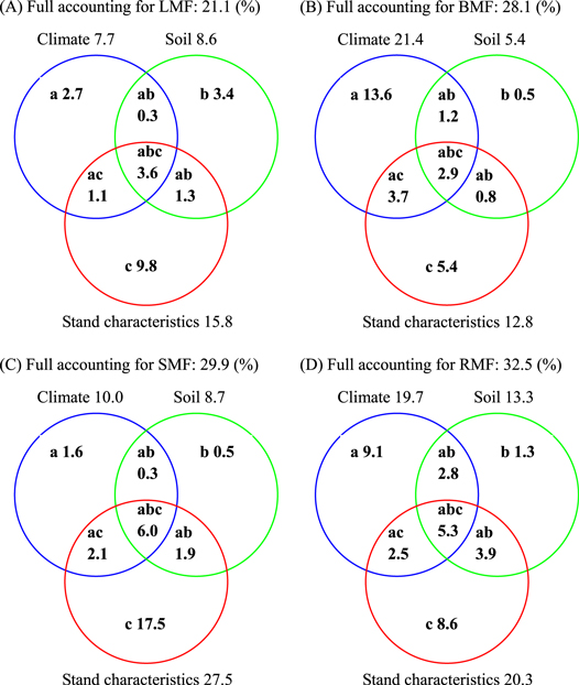
Partial general linear model (GLM) regressions could separate the variance explained by multiple factors into independent effects of all individual factors and interactive effects among factors (Legendre and Legendre 1998, Heikkinen et al 2005). The partial GLM performed in the current study revealed that the independent effects of climate were greater than those of soil chemistry and forest characteristics for BMF (figure 4). However, the independent effects of climate on LMF, SMF, and RMF were the largest, which suggests that the geography pattern of plant biomass allocation was largely controlled by forest characteristics. In addition, previous studies demonstrated how environmental factors affected forest biomass allocation; however, the role of interactions between environmental factors and forest characteristics has rarely been analyzed (Enquist and Niklas 2002, Hui et al 2014). In the current study, the interactions between forest characteristics, climate, and soil accounted for obviously portions of the variation in BAFs (figure 4).
Figure 4. Variation partitioning (r2) of environmental factors in accounting for the (a) LMF leaf mass fraction, (b) BMF branch mass fraction, (c) SMF stem mass fraction, and (d) RMF root mass fraction across forests in China. The symbols a, b, c represent the independent effects of climate, soil, and stand characteristics, respectively; ab is the interactive effect of climate and soil; ac, the interactive effect of climate and stand characteristics; bc, the interactive effect of soil and stand characteristics; and abc, the interactive effect of climate, soil and stand characteristics.
Download figure:
Standard image High-resolution image
The results of the current study do not support the isometric allocation hypothesis, which suggests that component biomass scale equivalently as total biomass across a diverse range of individuals from different plant species (Euquist and Niklas 2002, Niklas 2005) and community types (Cheng and Niklas 2007). In contrast, the BAFs varied with climate, soil chemistry, and forest types (tables 4 and 5). These results were consistent with some previous studies. For example, temperature drives global patterns in forest biomass distribution in leaves, stems, and roots (Reich et al 2014). R/S in forests varied with stand age, height, shoot biomass, precipitation, and temperature (Mokany et al 2006, Wang et al 2008, Luo et al 2012). However, the RMF data in this research are also inconsistent with some previous studies. For example, the belowground biomass scaled nearly isometrically with the aboveground biomass, and the scaling exponent did not vary by tree age, density, latitude, or longitude (Cairns et al 1997, Hui et al 2014).
The results of the current study can be explained in terms of optimal biomass allocation in response to environment (e.g. light, nutrients, water, and temperature). In forest communities, biomass allocation to stems, branches, and leaves all potentially increase the capture of light by trees (Dudley and Schmitt 1996, Poorter et al 2006). However, the costs (i.e. biomass allocation) and benefits (i.e. light capture) of stem, branch, and leaf growth differ (Poorter et al 2006). Nutrients and drought are the most complicated factors for the biomass allocation because there is no simple but objective way to characterize the severity of treatments (Poorter et al 2012). The response to severe drought is remarkable because plant biomass can be reduced by >50% compared with control plants, and RMF can be increased strongly (Deng et al 2006, Padilla et al 2009). Comparing for resource competition (e.g. light, nutrients, and water), low temperatures decrease the number of stems and leaves, and increase RMF (Zhou et al 2002). A variety of plant functions are also impaired by low temperature, including photosynthesis, nutrient uptake, and growth (Lambers et al 2008).
In addition, biomass allocation patterns are controlled by plant types and their interaction with stand dynamics and stand conditions, e.g. age, species mixture, competition etc (Zhang et al 2010, 2011). Within the group of woody species, there are different patterns of biomass allocation between deciduous and evergreen species (Poorter et al 2012). Higher allocation to roots and lower allocation to leaves in an evergreen forest will occur if higher leaf longevity is associated with infertile and/or dry sites (Givnish 2002). In a previous study, we also found that root biomass accumulation in Cyclobalanopsis glauca was more rapid in younger stands than in older stands (Zhang et al 2014), which is consistent with the current study (table 4). Moreover, plant biomass allocations can be affected by the interspecific or intraspecific competition as the result of the depletion of resources (Poorter et al 2012). For example, the research on plants competing for nutrients in split-root designs has shown that RMF increases when two plants rather than one are grown in twice the volume (Gersani et al 2001, O'Brien et al 2005).
Consistent with the above-mentioned studies, patterns of biomass allocation were affected by multiple environmental factors and forest characteristics in the current study (table 5). In addition to the above-mentioned influencing factors, management practices such as thinning, pruning, and fertilization might change biomass allocation in trees (Luo et al 2012, 2014). However, we did not analyze the effects of management practices in the current study, because management is a complex process with many unexplained variables. Moreover, although our data revealed that BAFs varied with climate, soil conditions, and forest types on a national level, the mechanism by which allocation is regulated remains poorly understood and source/sink relationships of all organs should be investigated in future studies (Poorter et al 2012).
4.3. Implications for estimates of C storage in China's forests
On a larger spatial scale, mean R/S is commonly calculated from published studies to quantify root biomass at the regional scale when only aboveground biomass is known (Brown et al 1993, Schroeder and Winjum 1995, Luo et al 2012). In this study, we compared forest type-specific R/S values that were calculated from the RMF of China's forests with those of global forests (Jackson et al 1996). The R/S of China's forests, which ranged from 0.11 to 0.35 (Luo et al 2012), were smaller than the global values of 0.18–0.70 (Cairns et al 1997). This suggests that China's forest C storage may be heavily overestimated if the global R/S values were used in calculations. Moreover, the large variation coefficients for BAFs suggest that the use of constant BAF values would lead to uncertain estimates of forest biomass and carbon. The results of the current study demonstrated that high variation in BAFs was related to climate (GST and GSP), soil chemistry, stand age, stand density, and forest types (figure 3; table 4), and these predictive BAF models for specific forest types by integrating climatic, soil and forest factors may help to predict accurately regional C sequestration and cycling under climate change. Finally, we are also aware that these predictive BAF models for specific forest types by integrating climatic, soil and forest factors is the first step toward the goal of improving accurately regional C sequestration and cycling under climate change. It is still needed to incorporate these predictive BAF models into terrestrial ecosystem C modeling in further research.
5. Conclusions
The current study reports that the geographical variability of biomass allocation fractions (BAFs) varies by climate conditions, soil chemistry and forest characteristics in China's major forest types. Whether the component biomass scales isometrically with total biomass across different forest ecosystems and along environmental gradients was tested at the community level. Data revealed that BAFs exhibit significant latitudinal, longitudinal and altitudinal trends, which are driven by significant influences of climate, soil chemistry, and forest characteristics. Stepwise multiple regression (SMR) models that involve the climate, soil, stand age and stand density show that these factors together account for a part of the biogeographical variation in BAFs and the explanatory power of these factors for different BAFs varied significantly. Reduced major axis (RMA) regression models indicated that BAFs differ in their environmental sensitivity (slope of their response to environmental gradients) to climate, soil and forest characteristics among the major forest types. Therefore, climate, soil and forest stand characteristics have a marked impact on biogeographical patterns of forest biomass allocation in China' forests. Our findings will help to better understand the relationship between BAFs, climate, soil chemistry, and stand characteristics, and are fundamentally important to policymaking and managing forest ecosystems to enhance the forest as a carbon sink.
Acknowledgments
This research was supported by the Chinese Academy Sciences Action Plan for the Development of Western China (KZCX2-XB3-10); Key State Basic Research Development Program of China (2015CB452703), the Strategic Priority Research Program-Climate Change: Carbon Budget and Related Issues of the Chinese Academy of Sciences (XDA05070404 and XDA05050205), the National Natural Science Foundation of China (nos. 31370485, 31370623, 31400412 and 41471233); the 100 Talents Program of the Chinese Academy of Sciences (2060299, Y251101111); the Western Light Program of Talent Cultivation of the Chinese Academy of Sciences and Guangxi Provincial Program of Distinguished Expert in China. The authors thank Hong-guang Zhu, Li-jun Zhao, You Nong, Jia-yan Wang, Tao Long, Wen-bo Li, Bei-si OuYang, De-xing Yuan, Guan-yi Qin, Wen-qing Dai, Li-su Wu, Yu Liu, Jia-hui Liao, Dan-hong Zhao, and Shu-yang Lin for help with data collection in the field.