

Abstract
Accurate estimation of forest aboveground biomass at high-resolution continues to remain a challenge and long-term goal for carbon monitoring and accounting systems. Here, we present an exhaustive evaluation and validation of a robust, replicable and scalable framework that maps forest aboveground biomass over large areas at fine-resolution by linking airborne lidar and field data with machine learning algorithms. We developed this framework over multiple phases of bottom-up monitoring efforts within NASA's Carbon Monitoring Program. Lidar data were collected by different local and federal agencies and provided a wall-to-wall coverage of three states in the USA (Maryland, Pennsylvania and Delaware with a total area of 157 865 km2). We generated a set of standardized forestry metrics from lidar-derived imagery (i.e. canopy height model, CHM) to minimize inconsistency of data quality. We then estimated plot-scale biomass from field data that had the closet acquisition time to lidar data, and linked to lidar metrics using Random Forest models at four USDA Forest Service ecological regions. Additionally, we examined pixel-scale errors using independent field plot measurements across these ecoregions. Collectively, we estimate a total of ∼680 Tg C in aboveground biomass over the Tri-State region (13 DE, 103 MD, 564 PA) circa 2011. A comparison with existing products at pixel-, county-, and state-scale highlighted the contribution of trees over 'non-forested' areas, including urban trees and small patches of trees, an important biomass component largely omitted by previous studies due to insufficient spatial resolution. Our results indicated that integrating field data and low point density (∼1 pt m−2) airborne lidar can generate large-scale aboveground biomass products at an accuracy close to mainstream lidar forestry applications (R2 = 0.46–0.54, RMSE = 51.4–54.7 Mg ha−1; and R2 = 0.33–0.61, RMSE = 65.3–100.9 Mg ha−1; independent validation). Local, high-resolution lidar-derived biomass maps such as products from this study, provide a valuable bottom-up reference to improve the analysis and interpretation of large-scale mapping efforts and future development of a national carbon monitoring system.
Export citation and abstract BibTeX RIS

Original content from this work may be used under the terms of the Creative Commons Attribution 3.0 licence. Any further distribution of this work must maintain attribution to the author(s) and the title of the work, journal citation and DOI.
1. Introduction
Forest carbon monitoring requires accurate estimates of aboveground biomass at high-resolution over large domains. Existing biomass maps are often inadequate for guiding such efforts because they have limited precision either by the spatial resolution (Blackard et al 2008b, Saatchi et al 2011, Saatchi et al 2012, Wilson et al 2013a) or by the geographical coverage (Huang et al 2013, Cook et al 2014). Although summary statistics from national to continental map products converge at continental scales (Avitabile et al 2016, Neeti and Kennedy 2016), discrepancies have been observed at local to regional scales when compared to high-resolution biomass maps (Huang et al 2015, 2017). Thus there is a critical need to develop a high-resolution map of forest biomass within the context of carbon monitoring over terrestrial ecosystems to assess ecosystem response to climate change (Houghton 2005, Houghton et al 2012, Gu et al 2016, Hurtt et al 2010, 2019), and to inform stakeholders at sub-regional to national scales to support policy-relevant activities such as Reduce Emissions Deforestation and Degradation (REDD+) and Paris Agreement (UNFCCC 2015).
Light Detection and Ranging (lidar) is the state-of-the-art remote sensing technology for forest carbon accounting because of its accuracy in measuring the height and three-dimensional canopy structures (Goetz and Dubayah 2011, Huang et al 2013, Lu et al 2014, Chen and McRoberts 2016). Improving biomass estimates with lidar and other remotely sensed data such as from multi-spectral images and Interferometry Synthetic Aperture Radar (InSAR) has been a subject of intense research with substantial advances in the last decades (Swatantran et al 2011, Saatchi et al 2012, Shendryk et al 2014, McRoberts et al 2018a, Zhao et al 2018). Increasing, lidar data are becoming available across large geographical scales, especially in the USA, Canada, and European countries. At statewide or nationwide scales, data from airborne lidar have been combined with field measurements such as those from Forest Inventory and Analysis database to assist stratified sampling and biomass estimation (Gregoire et al 2011), and produce wall-to-wall maps of forest structures and biomass (Gregoire et al 2011, Nord-Larsen and Schumacher 2012, Huang et al 2015, Chen and McRoberts 2016, Huang et al 2017, Nilsson et al 2017). For example, lidar data were used to map forest variables such as tree height and biomass for Denmark (Nord-Larsen and Schumacher 2012), Sweden (Nilsson et al 2017), and the State of Maryland (Huang et al 2015, Dubayah et al 2016), Sonoma County in California ( Duncanson et al 2017, Huang et al 2017,), and the State of Minnesota (Chen and McRoberts 2016) in the USA.
Yet challenges remain in the operational use of existing airborne lidar for statewide or nationwide seamless mapping (Lu et al 2014). These include but are not limited to differences in collection time, instruments type and parameters set up for lidar acquisitions and data format. Leaf-off lidar data, originally designed for producing seamless DEM, are increasingly available at regional to national scales (USGS 2018). However, these datasets are normally acquired through multiple flight campaigns in adjacent counties/states during winter time and distributed in varied data formats.
Other fundamental challenges include the definition of forest/non-forest areas, and uncertainties in tree allometry and field measurements (Huang et al 2015). Different definitions of forest and non-forest could lead to large discrepancies when comparing local-scale mapping results to national-scale products (Huang et al 2015, 2017). Choice of national or local tree allometry could resulted in as much as 20% difference in field estimates of biomass and similar level of difference in county level estimates built upon lidar data (Duncanson et al 2015, 2017). Last but not least, the uncertainties arose from the empirical relationships between field-measured biomass and lidar variables (McRoberts et al 2018a).
In this paper, we developed a framework that quantifies forest aboveground biomass over large geographical areas at high-resolution using lidar and field measurements. We combined forest attributes such as tree canopy cover and canopy structures predicted from leaf-off lidar data with field measurements to estimate biomass in both natural, planted and urban forests. In the process, we evaluate our maps rigorously with both with-held and independently collected plot data and discuss factors affecting our model predictions and the spatial patterns of resulting maps. This bottom-up approach at regional-scale complements the top-down continental-scale mapping to form a comprehensive carbon monitoring system (CMS).
2. Data and method
We combined existing field plots, wall-to-wall lidar, and optical data. The field data were used with allometry to estimate plot level biomass. The remote sensing data were used with a subset of these field estimates of biomass to drive machine learning models. In general, our framework has four general steps: (1) field data preparation, (2) remote sensing data processing, (3) model development and mapping, and (4) map validation and error analysis (figure 1).
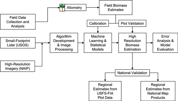
Figure 1. Diagram shows modeling and validation framework.
Download figure:
Standard image High-resolution image2.1. Study area and field data
The study area, Tri-State region of Pennsylvania (PA; 119 280 km2), Maryland (MD; 32 133 km2), and Delaware (DE; 6452 km2) in the USA (hereafter Tri-State region) covers a land area of approximately 157 865 km2. The Tri-State region contains four major ecological regions that are generally uniform with respect to species-composition and environmental gradients (figure 2). These regions are the Outer Coastal Plain Mixed, Eastern Broadleaf, Central Appalachian Broadleaf-Coniferous, and Northeastern Mixed Forest, adapted from Bailey's ecoregions for the Conterminous United States (Bailey 1995). Forests, including woody wetlands, comprise 56% of the total area based on National Land Cover Dataset (NLCD) 2011 (Homer et al 2015). The topography varies substantially with elevations ranging from about sea level near the Delaware River to 1027 m in Western Maryland.
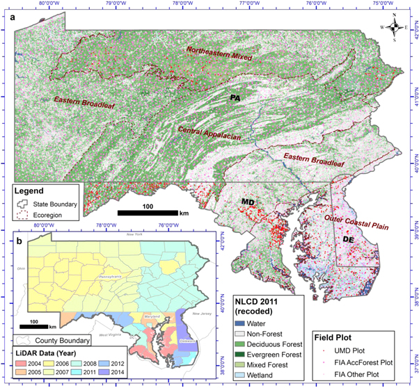
Figure 2. Study area shows mean canopy height and field plot locations (a), and map of lidar acquisition dates colored by year (b). The height classes (5–10 m intervals) are taken from the average-maximum height, which was derived from maximum height in 10 m cell and then averaged to 30 m. FIA plots (location perturbed for privacy) were measured from year 2009 to 2013 in Maryland and Delaware, and measured from year 2005 to 2009 in Pennsylvania. UMD plots were measured from year 2011 to 2016.
Download figure:
Standard image High-resolution imageThe field data collected over the domain is built from two sections: USDA forest inventory analysis (FIA) plot data for model development, and independent field measurements collected by the University of Maryland (UMD) for product validation. For this study, 2243 forest plots that most closely matched the lidar year of acquisition over the domain were extracted from the FIA database (EVALIDator Version 1.6.0.03a). These plots, consist of measurements for individual tree height, diameter and species, were collected from year 2004 to 2013 in MD and DE, and from year 2005 to 2009 in PA, 92% of them had a less than 2 years difference (supplement S2 and table S2 is available online at stacks.iop.org/ERL/14/095002/mmedia).
Additionally, a total of 1163 variable-radius plots (VRP) were collected by UMD plots) between 2010 and 2013 in MD (Dubayah 2012, Huang et al 2015), in the summers of 2014 and 2015 for the northeastern forest in PA and DE, respectively. VRP locations were determined by a modified random stratified sampling scheme broken down by ecoregions (Bailey 1995), NLCD 2011 land cover classes (Home et al 2015), and lidar canopy height (figure 2). Individual tree species, dbh and maximum height were measured in the field.
Plot-level aboveground live biomass was estimated using allometric models. For the sake of comparison with different map products, two types of allometric relationships were prepared: (1) regional models from FIA's Component Ratio Method (CRM) (Heath et al 2008, Woodall et al 2011) and (2) national generalized models (JKS) from Jenkins et al (2003). County and state scale total biomass was calculated based on sample probability for each allometric equation (FIAcrm and FIAjks).
Lastly, both the FIA and UMD plot data were screened for outliers. The screening omitted plots located in no lidar data areas (i.e. missing tiles in Maryland) and excluded mismatched plots between biomass and lidar heights with three filtering rules: had zero biomass but lidar heights (>10 m); had large biomass (>500 Mg ha−1) but low lidar heights (<10 m); and small biomass (<50 Mg ha−1) but high lidar heights (>30 m). These filters reduced the number of FIA plots from 2243 to 2215, and the number of UMD plots from 1163 to 1046. Summary statistics of the FIA and UMD plots are given in table 1.
Table 1. Summary of field data: (a) FIA plots, and (b) UMD plots. Areal distributions on four ecoregions, corresponding field plot numbers, maximum tree height and estimated live aboveground biomass on the plots.
| (a) FIA plot | (b) UMD plot | ||||||||||
|---|---|---|---|---|---|---|---|---|---|---|---|
| Variable (unit) | Ecoregion | n | Min. | Max. | Mean | SD | n | Min. | Max. | Mean | SD |
| Maximum tree height (m) | Central Appalachian | 739 | 0.0 | 40.2 | 16.1 | 5.7 | 311 | 0.0 | 40.3 | 18.3 | 12.0 |
| Eastern Broadleaf | 481 | 0.0 | 44.5 | 17.2 | 6.1 | 156 | 0.0 | 46.1 | 20.9 | 10.3 | |
| Northeastern Mixed | 796 | 0.0 | 42.7 | 18.3 | 5.3 | 165 | 0.0 | 36.6 | 22.8 | 7.3 | |
| Outer Coastal Plain | 199 | 0.0 | 45.7 | 16.8 | 6.9 | 531 | 0.0 | 43.9 | 21.0 | 11.7 | |
| Total | 2215 | 0.0 | 45.7 | 17.2 | 5.9 | 1163 | 0.0 | 46.1 | 20.5 | 11.1 | |
| Live biomass (Mg ha−1) | Central Appalachian | 739 | 0.0 | 370.5 | 140.3 | 68.0 | 311 | 0.0 | 616.0 | 112.0 | 129.8 |
| Eastern Broadleaf | 481 | 0.0 | 428.0 | 137.0 | 81.5 | 156 | 0.0 | 623.0 | 146.9 | 135.6 | |
| Northeastern Mixed | 796 | 0.0 | 437.8 | 154.4 | 70.5 | 165 | 0.0 | 496.5 | 197.5 | 116.8 | |
| Outer Coastal Plain | 199 | 0.0 | 432.3 | 153.5 | 84.9 | 531 | 0.0 | 591.0 | 149.6 | 128.0 | |
| Total | 2215 | 0.0 | 437.8 | 145.8 | 74.0 | 1163 | 0.0 | 623.0 | 146.0 | 130.7 | |
2.2. Data processing for lidar and auxiliary data
Discrete return lidar data were collected through different county and state government agencies (summarized in supplement S2 and table S1) over the Tri-State region (figure 2(b)). These airborne lidar collections were originally dedicated to surveying digital elevation model (DEM). Therefore leaf-off season (December–January) were picked for flight. Lidar first returns were interpolated into digital surface model (DSM); last returns were utilized to derive a bare earth DEM using quick terrain modeler and other GIS-based software (O'Neil-Dunne et al 2013, 2014). Then DSM and DEM were differenced to obtain a normalized difference surface model (nDSM).
High-resolution tree canopy cover map at 1 m resolution for circa 2011 over the domain was created using an object-based approach that integrated the lidar data and high-resolution multi-spectral images from the National Agricultural Imagery Program or NAIP (O'Neil-Dunne et al 2013, 2014, USDA 2018, supplement S3). A canopy height model (CHM) was then extracted by applying the canopy cover mask to the nDSM, thereby creating a height model that excluded non-canopy height.
The definition of tree canopy used for high-resolution [1 m] product was a minimum height of 2.5 m and a minimum area of 4 m2. This definition is wider than the FIA definition of forest, which only refers to forested areas that are not developed for nonforest land uses, at least an acre in size and 120' in width, and contain a live plus missing canopy cover of at least 10% (USFS 2018a).
A set of percentage canopy cover and mean canopy height maps were generated from aggregating the 1 m tree canopy cover and tree height maps. The percentage tree canopy cover was aggregated to 30 m. From the CHM, the max tree height within each 10 m cell was first calculated and then averaged to 30 m resolution (hereafter referred to as average-maximum height).
A set of forestry metrics were prepared, including percentile heights, density metrics, mean heights, canopy covers, and topographical indices (table 2). Specifically, metrics were calculated at plot-scale and pixel-scale for modeling and mapping purpose. At plot-scale, we located the extent of a given plot using the plot centroid and calculated metrics within a given size of plot (e.g. 30 m). These metrics have been found high correlated with biomass (Goetz and Dubayah 2011, Swatantran et al 2012, Huang et al 2013, Whitehurst et al 2013, Zhao et al 2018, Hurtt et al 2019), shown in figure S2. At pixel-scale, we calculated metrics at 30 m resolution for each pixel within the domain. Countywide maps were created first and merged into a seamless statewide map aligned to a common extent.
Table 2. Definition of lidar and topographical metrics used in this study.
| Type | Metrics | Descriptions |
|---|---|---|
| Lidar metrics | P05, P10, ... P95, P100; | Percentile heights, in meter. Divide height range between ground (>0 m) and maximum height (P100) in given cell into 20 equal vertical height bins. |
| D05, D10, ... D95, D100; | Density percentiles or 'bincentiles', in percentage. Divide the percentage of height between canopy (2.5 m) and P100 in given cell into 20 equal vertical height bins. Deliver the accumulated percentage of pulses above a given height from top down. | |
| PERCT_CA, PERCT_CC; | Canopy crown closures, in percentage. For all pulses (CA), and for canopy hits only (CC). | |
| QMHA, QMHC; | Quadratic mean heights, in meter. For all pulses and canopy hits only. QMH = sqrt [(sum (squared heights)/n)]. | |
| HTA, HTC, HTM; | Mean heights, in meter. For all pulses (HTA), canopy heights above 2.5 m (HTC), and average maximum 10 m height (HTM). | |
| SDA, SDC; | Standard deviation of HTA and HTC. | |
| Topographical variables | slope, aspect; | Average slope and aspect extracted from DEM. |
Four national and a global scale biomass maps were prepared for map comparisons, summarized in table 3. The national biomass and carbon dataset (NBCD) 2000 was the first 30 m national product developed using medium resolution satellite optical imagery from Landsat enhanced thematic mapper plus (ETM+) and InSAR data from shuttle radar topography mission (SRTM) (Kellndorfer et al 2012). Two versions of the NBCD biomass maps were extracted for consistency with other national maps, including the FIA database version using CRM for allometry (NBCDcrm) and the nationally consistent allometric models (NCE) version using JKS allometry models (NBCDjks). The Saatchi map is a 90 m national-scale biomass map generated using optical, radar and lidar data and forest inventory data (Saatchi et al 2012). Both the Blackard and Wilson were 250 m national biomass datasets generated by USDA forest service two generated by USFS (Blackard et al 2008a, 2008b, Wilson et al 2013b). The GlobBiomass map was a 100 m global biomass product converted from growing stock volume (Santoro 2018). Detailed descriptions for these maps are given in supplement S6.
Table 3. Summary of biomass product compared in this study.
| Product | Norminal Year | Sensor and Year | Field data and Year | Resolution | Forest mask | Approach | Uncertainty map | References |
|---|---|---|---|---|---|---|---|---|
| RFjks | 2011 | DRL 2004–2012 | 2011–2014 | 30 m | NAIP high-res tree canopy cover | Random forest | Percentile error (QRF) | Huang et al (2015), Dubayah et al (2018) |
| NBCD | 2000 | Landsat+SRTM 2000 | 2000 | 30 m | NLCD 2001 | Random forest, two-steps | Quality voids | Kellndorfer et al (2012) |
| Blackard | 2001 | MODIS 2001a | 2005–2009 | 250 m | NLCD 1992 | Cubist, two-steps | Relative error | Blackard et al (2008a), (2008b) |
| Wilson | 2005 | MODIS 2002–2008 | 2005–2009 | 250 m | NLCD 2001 percent tree canopy 25% | Imputation, two-steps | Not reported | Wilson et al (2013a) |
| Saatchi | 2005 | MODIS+ PALSAR+ Landsat | 2005 | 90 mb | NLCD 2006 | MaxEntropy, parametric | Percent error | Saatchi (2012) |
| GlobBiomass | 2010 | SAR, lidar, optical | 2000 | 100 mc | Hansen et al (2013) percent tree cover 0% | Rule-based combination of different algorithms | Standard error | Santoro (2018) |
aYear is for national maps in eastern US. bOriginal maps are in lat/lon with 0.00083333° ≈ 90 m. cOriginal maps are in lat/lon with 0.00089999° ≈ 100 m.
For forest mask, the National Land Cover Dataset or NLCD 2011 (30 m) (Homer et al 2015) were utilized to differentiate between forested and non-forested areas for map comparisons. Specifically, woody forestlands (deciduous, conifers and mixed) and woody wetlands were included as forested area. From the NLCD forest mask, we applied a 20% threshold to aggregate the mask from 30 to 250 m. For consistency and statistical measurement purposes, all biomass and land cover maps were projected into Albers Equal-area Conic projection. All pixels were aligned to NLCD 2011 30 m cell.
2.3. Statistical models calibration
Random Forest models were developed using 80% of FIA plots to predict field-estimated biomass as a function of forestry and topographical metrics. Quantile Regression Forests (QRF), which predicts a particular quantile (10% and 90%), was employed to provide model error bounds (Meinshausen 2006). The R packages 'randomForest' and 'quantregForest' were used for modeling analyses (Liaw and Wiener 2002, R Development Core Team 2016). We employed several statistical measurements such as coefficient of determination (R2), root-mean-squared error (RMSE), RMSE CV (%), and mean estimated bias error (MBE) to validate results at plot-scale.


where xi is the value from field measurements, yi is the predicted value from RF model; i is the sample index; and  and
and  are the means of field measurements and predicted values respectively; and n is the sample size.
Models developed for each ecoregion were applied to make countywide predictions for a total of 94 counties. Specifically, Outer Coastal model was applied to 16 counties, Eastern Broadleaf model was applied to 31 counties, Central Appalachian model was applied to 21 counties, and Northeastern Mixed model was applied to 26 counties. Details about random forest models were given in supplement S2.
Lastly, county-scale mean biomass density (Mg ha−1) and biomass stock (Tg) over DE, MD, and PA were summarized using average and sum methods. The Maryland canopy height map had gaps comprising around 1.5% of the state because of data collection restrictions and quality issues. To overcome this, these data gaps were filled with values from the NBCD product. Specifically, the height values were from weighted basal area heights (NBCD_BAW) and biomass values were from the national consistent allometry equation version of biomass (NBCDjks) (Huang et al 2015).
2.4. Plot-scale validation and error analysis
At the plot-scale, we compared estimates of biomass density from this study (RFjks) to with-held FIA plots and UMD plots. Explicitly, we conducted plot-scale validation using the 20% with-held FIA plots. Then, we used all UMD plots as independent plot-scale validations. In addition, we test the scale effect by comparing the RF predicts from 30 m and 90 m metrics to estimates from FIA plots (supplement S2). Maps of uncertainty were generated for every 30 m pixel. RF predicts the mean response for any given location. Prediction intervals were developed using QRF. QRF is similar to RF but it retains all responses and allows for constructing prediction intervals. We generated the 10th and 90th prediction percentiles and analyzed the spatial distribution of errors across the state. The uncertainty index is calculated as:

where yi is the predicted value from RF model; Perct10i and Perct90i are the predicted values from 10th and 90th prediction percentiles, respectively.
2.5. National map validation
Estimates of biomass from this study (RFjks) were compared to four national and one global products (NBCDjks, Saatchi, Blackard, Wilson, and GlobBiomass) at the pixel, county and state scales following the framework we setup in previous studies in Maryland and California (Huang et al 2015, 2017).
At the pixel scale, we compared biomass maps at 250 m spatial resolution, the coarsest resolution among all maps in this study. We choose to use this resolution because previous analysis found that the map comparisons at coarser resolution are more reliable (Huang et al 2017). The aggregation process reduces the difference caused by geolocation and misalignment between different maps. Statistical measurements such as R2, root-mean-squared difference (RMSD, calculated similar to RMSE) and mean estimated bias difference (MBD, calculated similar to MBE), were selected to evaluate results at pixel-scale.
At the county to the state scale, we compared estimates from five map products to FIA estimates. Especially, we compared the map-based county and state-scale estimates of aboveground biomass from this study, four national products (NBCDjks, Saatchi, Wilson, and Blackard), a global product (GlobBiomass) and sample-based estimates from FIA plots using two different allometric equations (FIAjks and FIAcrm). Additionally, at the state- to Tri-State region scales, we compared estimates of mean carbon density and stock from map-based results to sample-based estimates from FIA. A coefficient of 0.5 was used to convert from biomass to carbon (Chave et al 2005). We used similar statistical indicators (i.e. R2, RMSE, and MBE) as described in section 2.3 to evaluate the map-based results.
3. Results
3.1. Statewide forest biomass products
Visually, the spatial patterns of canopy cover, mean canopy height and biomass matched land cover and topography (figure 3). In general, counties in western Maryland and northern Pennsylvania had the highest mean canopy heights, largest forest cover, and total and mean biomass. The Blue Ridge region had large biomass while the coastal plains had smaller biomass in general. Biomass distribution was patchy and heterogeneous as expected from the patchy nature of the landscape. The map of uncertainty index derived from QRF models shows similar spatial patterns matched canopy cover and height (figure S2).
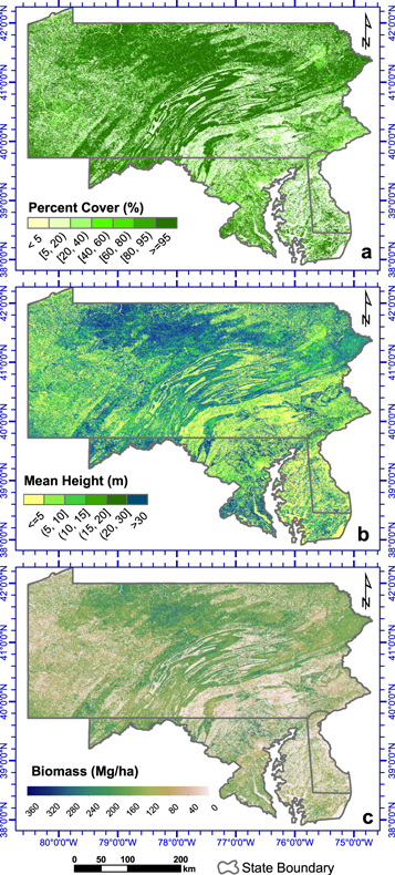
Figure 3. Statewide percent tree canopy cover (a), mean canopy height (b), and biomass density (c) at 30 m spatial resolution over Tri-State region of Maryland, Pennsylvania, and Delaware.
Download figure:
Standard image High-resolution imageHigh-resolution maps reveal more details (figure 4). The canopy cover map at 1 m resolution detailed delineating out important urban forests that traditionally defined as 'non-forest', such as open, low and medium high developed land cover types. The canopy height map revealed not only the extent of forest but also vertical information, which is critical for estimating carbon in forests. Larger biomass values were observed in urban areas that have tall trees and residential neighborhoods that have tree plantation programs (figure S6(a)). Biomass values were larger near water bodies, as canopy heights were higher in protected wetlands (figure S6(b)).

Figure 4. Comparison of Random Forests predicted and field estimated biomass from calibration dataset (a) (FIA 80% data) and validation dataset (b) (FIA 20% with-hold data). From left to right are results from each ecoregion: Outer Coastal Plain Mixed, Eastern Broadleaf, Central Appalachian Mixed, and Northeastern Mixed.
Download figure:
Standard image High-resolution image3.2. Plot-scale validation and error analysis
Plot-scale validation of biomass density showed different levels of agreement when using FIA plots (figure 4) and UMD plots (figure S4). The Random Forest models explained moderate variability in biomass from FIA plot data (R2 = 0.46–0.54, RMSE = 51.4–54.7 Mg ha−1, RMSE CV = 34.1%–39.9%) with small estimated biases (MBE = 4.2–12.7 Mg ha−1) (a). These values are slightly better than RMSE values reported by NBCDjks, ranged between 52.0 and 58.0 Mg ha−1 (i.e. 5.2–5.8 kg m−2) in their bootstrap validation for five mapping zones (zone 60 to zone 64) that covers the study area. Unexpectedly, we noticed saturation effects in all ecoregion models. Validation using 20% with-held FIA plots indicated that four ecoregion models performed differently (b). Independent validation using UMD plots (figure S3) showed larger errors (R2 = 0.33–0.61, RMSE = 85.3–100.9 Mg ha−1, RMSE CV = 43.2%–85.0%) and different scales of under estimations (MBE = −8.9 ∼ −45.5 Mg ha−1), but followed similar patterns as the results using FIA plots.
Similar patterns in biomass distribution were found when comparing the RF products from 30 and 90 m metrics to estimates from FIA plots (figure S5). Two of the four ecoregion models (Eastern Broadleaf and Northeastern Mixed) have smaller estimated biases in biomass predictions (MBE = 0.6–1.6 Mg ha−1) using metrics generated at 30 m or 90 m scales. While the other two ecoregion biomass models had either underestimation (Outer Coaster, MBE = −17.4 Mg ha−1) or overestimation (Central Appalachian, MBE = 11.6 Mg ha−1) when using metrics at 30 m scales.
3.3. Comparison to existing products
The random forest derived biomass map (RFjks) was compared to four national products (NBCD, Saatchi, Blackard, Wilson) and one global map product (GlobBiomass) over the Tri-State region. Although all map products followed general patterns in topography and landscape, fine-scale details varied especially over urban fringes (figure 5). Over forested area, less disagreements were observed among the three finer scaled map products (NBCDjks 30 m, Saatchi 90 m and GlobBiomass 100 m) and RFjks, compared to larger disagreements found among the two coarser map products (Wilson and Blackard, 250 m) and RFjks, as illustrated in the scatter plots and associated errors (figure 6). Biomass estimates had stronger correlations (R2 > 0.65) among the three InSAR-optically fused national maps (NBCDjks, Saatchi and GlobBiomass) and the RFjks map over all regions. The two coarser resolution maps (Wilson and Blackard) had the poorest agreement with the RFjks.
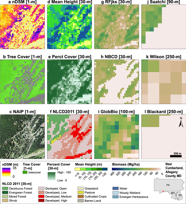
Figure 5. Fine scale map example of spatial variation in biomass density over an urban fringe area near Cumberland in Allegany County, Maryland. (a) DEM (10 m), (b) NLCD 2011 (30 m), (c) NAIP (1 m), (d) Canopy Cover (1 m), (e) NLCD forest (30 m), (f) Combined forest (30 m), (g) RFjks (30 m), (h) NBCDjks (30 m), (i) GlobBiomass (100 m), (j) Saatchi (90 m), (k) Wilson (250 m), and (l) Blackard (250 m).
Download figure:
Standard image High-resolution image
Figure 6. Density scatter plots showing pixel-scale comparison of biomass density from four national and one global maps versus results from this study. From upper to bottom panels, are: (a) NBCD, (b) Saatchi, (c) GlobBiomass, (d) Wilson, and (e) Blackard. From left to right columns, are comparisons over: total area, forested and non-forested area. The x-axis in each plot represents biomass values from this study (RFjks), and the y-axis represents biomass values from each map product. The forest/non-forest mask is derived from the 30 m NLCD 2011.
Download figure:
Standard image High-resolution image
The relationships at county- and state-scale varied between biomass estimates among five map products and those produced by the USFS FIA for the Tri-State region (table 4). All map-based estimates agreed well with the FIA estimates at county-scale (R2 > 0.92, RMSD ranged between 3.0 and 9.0 Tg; figure S6). Details in county-scale of biomass density and stock were illustrated in figures S7 and S8. At the state-scale, the estimated aboveground biomass among different maps and USFS FIA showed large differences over forest and non-forest area. In Pennsylvania and Tri-State region (PA dominated), the four map-based estimates (RFjks, NBCDjks, Saatchi and GlobBiomass) that used either lidar or InSAR derived variables as model predictors, achieved closer values to each other as well as to the FIAjks over forest regions, but were more diverse over non-forest regions. In Maryland and Delaware, the estimates from this study (RFjks) matched best to FIA estimates over forest regions, followed by the estimates from the other three finer scaled maps (NBCDjks, GlobBiomass, and Saatchi). The estimated aboveground carbon density and stock among different maps and USFS FIA estimates showed large differences for each state and the Tri-State region. The map-based estimates in aboveground biomass ranged between 527.5 and 680.2 Tg across the Tri-State region. Whereas the USFS FIA estimates ranged between 638.4 (CRM) and 695 (Jenkins) Tg. Our estimates in aboveground carbon (563.8, 103.4 and 13 Tg) matched best to USFS for Pennsylvania, Maryland and Delaware (562.4, 116.7 and 15.9 Tg). The carbon estimates from the two coarser maps (Wilson & Blackard) were consistently ∼20% less than FIAcrm estimates in forested areas.
Table 4. Estimates of aboveground carbon density (Mg C ha−1) and carbon stock (Tg C) in forest from this study (RFjks), four national and one global map products, and FIA estimates (FIAjks and FIAcrm) over (a) All, (b) Forested, and (c) Non-Forest area summarized by states and the Tri-State region. RFjks, NBCDjks and FIAjks represent estimates using Jenkins allometry. RFcrm, NBCDcrm and FIAcrm represent estimates using CRM allometry.
| Maryland | Delaware | Pennsylvania | Tri-State | |||||
|---|---|---|---|---|---|---|---|---|
| (a) Total | Density | Stock | Density | Stock | Density | Stock | Density | Stock |
| RFjks | 42.5 | 103.4 | 27.5 | 13.0 | 53.4 | 563.8 | 50.5 | 680.2 |
| %diff2FIA | 7.6% | −11.4% | −18.5% | −18.3% | 0.3% | 0.3% | 8.7% | −2.1% |
| NBCDjks | 35.3 | 85.9 | 24.5 | 11.6 | 54.0 | 570.2 | 44.6 | 667.7 |
| %diff2FIA | −10.6% | −26.4% | −27.4% | −27.1% | 1.4% | 1.4% | −4.0% | −3.9% |
| Saatchi | 38.2 | 92.8 | 26.9 | 12.7 | 54.3 | 517.2 | 45.4 | 678.8 |
| %diff2FIA | −3.3% | −20.5% | −20.2% | −20.2% | 2.0% | −8.0% | −2.3% | −2.3% |
| GlobBiomass | 40.7 | 99.0 | 24.5 | 13.0 | 52.1 | 550.3 | 44.3 | 662.3 |
| %diff2FIA | 3.0% | −15.2% | −27.4% | −−18.3% | −2.2% | −2.1% | −4.6% | −4.7% |
| FIAjks | 39.5 | 116.7 | 33.7 | 15.9 | 53.2 | 562.4 | 46.5 | 695.0 |
| Wilson | 33.0 | 80.1 | 25.3 | 11.9 | 45.0 | 464.1 | 37.9 | 566.8 |
| %diff2FIA | −14.3% | −25.0% | −16.8% | −16.9% | −8.2% | −10.3% | −11.2% | −11.2% |
| Blackard | 26.8 | 65.2 | 17.3 | 8.2 | 43.0 | 454.1 | 35.3 | 527.5 |
| %diff2FIA | −30.4% | −39.0% | −43.0% | −43.1% | −12.2% | −12.2% | −17.3% | −17.4% |
| FIAcrm | 38.5 | 106.9 | 30.4 | 14.3 | 49.0 | 517.2 | 42.7 | 638.4 |
| (b) Forest | ||||||||
| RFjks | 70.2 | 75.9 | 60.1 | 8.8 | 66.4 | 473.9 | 66.8 | 558.7 |
| %diff2FIA | −27.2% | −19.1% | −40.2% | −33.4% | −16.3% | −6.9% | −0.2% | −9.3% |
| NBCDjks | 68.1 | 73.6 | 65.3 | 9.6 | 74.1 | 528.6 | 73.2 | 611.8 |
| %diff2FIA | −29.4% | −21.5% | −35.0% | −27.4% | −6.6% | 3.8% | 9.3% | −0.7% |
| Saatchi | 67.4 | 72.9 | 63.6 | 9.3 | 70.8 | 573.3 | 70.2 | 587.1 |
| %diff2FIA | −30.1% | −22.3% | −36.7% | −29.7% | −10.8% | 12.6% | 4.8% | −4.7% |
| GlobBiomass | 67.0 | 72.4 | 60.6 | 8.9 | 65.6 | 467.6 | 65.7 | 548.9 |
| %diff2FIA | −30.5% | −22.8% | −39.7% | −32.7% | −17.3% | −8.2% | −1.9% | −10.9% |
| FIAjks | 96.4 | 93.8 | 100.4 | 13.2 | 79.3 | 509.3 | 67.0 | 616.3 |
| Wilson | 46.1 | 49.8 | 40.2 | 5.9 | 52.9 | 377.0 | 51.8 | 447.8 |
| %diff2FIA | −46.5% | −40.6% | −54.6% | −49.6% | −26.8% | −18.8% | −22.7% | −20.0% |
| Blackard | 46.4 | 50.2 | 37.5 | 5.5 | 55.0 | 392.1 | 53.6 | 447.8 |
| %diff2FIA | −46.2% | −40.2% | −57.7% | −53.0% | −23.9% | −15.5% | −20.0% | −20.0% |
| FIAcrm | 86.2 | 83.9 | 88.6 | 11.7 | 72.3 | 464.1 | 67.0 | 559.7 |
| (c)Non-Forest | ||||||||
| RFjks | 16.9 | 27.5 | 11.0 | 4.2 | 19.5 | 89.8 | 18.4 | 121.5 |
| %diff2FIA | 15.9% | 26.9% | 10.2% | 11.3% | 8.4% | 7.2% | 14.3% | 10.3% |
| NBCDjks | 7.6 | 12.3 | 5.3 | 2.0 | 9.1 | 41.6 | 8.5 | 56.0 |
| %diff2FIA | 6.2% | 10.7% | 4.5% | −5.3% | −4.7% | −2.3% | −0.4% | −0.3% |
| Saatchi | 12.3 | 20.0 | 9.0 | 3.4 | 14.8 | 505.0 | 13.9 | 91.7 |
| %diff2FIA | 11.1% | 18.9% | 8.2% | 5.3% | 2.5% | 88.7% | 7.6% | 5.5% |
| GlobBiomass | 16.3 | 26.5 | 11.1 | 4.2 | 18.0 | 82.8 | 17.2 | 113.5 |
| %diff2FIA | 15.2% | 25.8% | 10.3% | 11.3% | 6.6% | 5.8% | 12.5% | 9.0% |
| FIAjks | 1.6 | 2.3 | 0.8 | 2.7 | 12.8 | 53.1 | 8.8 | 58.1 |
| Wilson | 18.7 | 30.3 | 16.0 | 6.0 | 21.2 | 97.7 | 20.3 | 134.1 |
| %diff2FIA | 13.9% | 24.3% | 17.5% | 37.6% | 14.2% | 11.3% | 17.5% | 13.8% |
| Blackard | 9.2 | 15.0 | 7.1 | 2.7 | 13.5 | 62.0 | 12.1 | 79.7 |
| %diff2FIA | 2.9% | 6.1% | 7.4% | 9.4% | 3.6% | 3.6% | 5.2% | 4.1% |
| FIAcrm | 6.7 | 9.9 | 0.5 | 1.6 | 10.9 | 45.2 | 8.6 | 56.6 |
4. Discussion
Combining lidar derived metrics and auxiliary data, and FIA plots, the RF models were calibrated, applied and validated for estimating biomass over Tri-State region. Validation of biomass estimates at FIA plot-level using with-hold data showed similar levels of expiation and associated errors as RF training data. Although independent validation using finer scale UMD plots indicated consistent negative biases, the biomass map from this study reveals more details at finer scales. Additionally, map comparison between existing products and this study indicated that biomass estimates from InSAR-optically fused products (e.g. NBCDjks, Saatchi, and GlobBiomass) generally agree better with our map (RFjks) over forested.
Our estimates of biomass have uncertainties that arose from several factors. One uncertainty in our biomass product is caused by using leaf-off lidar data that have relatively low point density. In this study, we utilized many archived lidar data (e.g. Pennsylvania and several counties in Maryland) that have less than 1 pt m−2 as well as newly collected higher-quality lidar data (i.e. Delaware and a few counties in Maryland). Studies had indicated lidar tends to underestimate actual heights with decreasing point density (more likely to miss the canopy top), and suggested to further normalize by integrating CHM to coarser resolutions (e.g. 5 m) (Zhao et al 2018). We also used maximum canopy height at 10 m resolutions and integrated into 30 and 90 m mean max canopy height metrics (Max10Avg), which was expected to dampen much of the low sampling effect. This mean height metric as expected was always among the best predictors (figure S3). However, lidar measured canopy height and canopy cover were only moderately correlated with biomass and with the best metrics explaining around 30%–40% variability of biomass in general (figure S2). These findings suggested that the ability of lidar data in predicting biomass are limited in certain regions, particularly in eastern temperate broadleaf and mixed forests and urban forests with widely varying management and growth patterns.
A second major uncertainty arose from the allometric models and carbon fraction used in biomass and carbon estimation. A study over the mixed forests of Sonoma County, California indicated that the choice of local or national allometric models (CRM versus Jenkins) resulting in a 20% difference in biomass estimates at plot to county scales (Duncanson et al 2017). Further, the complexities associated with quantifying biomass accurately with lidar in northeastern temperate broadleaf and mixed forests are increasing acknowledged (Anderson et al 2008, Huang et al 2015, Weiskittel et al 2015). Two recent studies indicated insufficient sampling for the parameterization of allometric models leads to bias in these temperate forests (Duncanson et al 2015, Weiskittel et al 2015). Our research concurred with this and also showed that at sub-hectare plot scales, there was such a wide variability in basal area for a given tree height that it is very difficult to predict biomass with more than 60% variability (figure S1) with three-dimensional structure and height from airborne lidar with low point density (∼1 pt m−2). However, this is not to say that the results cannot be enhanced with greater datasets. Such improvement would require a better knowledge about the allometric relationship between biomass and forest structure from field survey, potentially available from recent advances in terrestrial laser scanning (Liang et al 2016). In addition, a consistent fraction (0.5) was used when converting biomass to carbon, which may overestimate carbon in angiosperms in the Tri-State region (Martin et al 2018). Alternatively, we would expect to improve results by testing refined stratification over the study area in our future study.
Third, uncertainty occurred because of the mismatch and time lag between lidar metrics and field measurements. For instance, the lidar metrics were calculated at 30 m equivalent pixels (i.e. a square size) for mapping purposes, but the field measurements were taken in different ways. The FIA plot data were sampled using a four-subplot methodology, not all the trees within the whole plot were measured. Our independently collected UMD plots were measured using a mixture of variable and fixed radius methods (Huang et al 2015). Although preliminary comparisons between variable and fixed radius plots did not show a substantial difference in model performance (Dubayah 2012), we found errors were introduced because of the complexity and heterogeneity in the landscape as well as partial alignment of plots and lidar data. Additionally, due to lack of coincident field and lidar data, we used FIA plot that have time lags with lidar data. Only 20% of the FIA plot were measured in the same acquisition year as lidar data, while 72% and 8% of the FIA plots have 1–2 and 3–5 year time differences, respectively (table S2). The Outer Coaster ecoregion model had the largest time difference, where 36.2% of the FIA plot had a 3–5 year difference, showed an underestimation (MBE = −17.4 Mg ha−1) in the independent validation using UMD plot. However, the mismatch and associated errors were reduced when estimates were scaled-up and comparing results at county-scale. These findings are consistent with another recent study (McRoberts et al 2018b).
Lastly, the varied definition of forest/non-forest among different forest cover, biomass and carbon products have made the comparison between different products difficult. Traditionally, the FIA program did not consider plots located in urban regions that had some forest cover, resulting in a possible underestimation in carbon from urban forests (Johnson et al 2014, 2015). For example, there are approximately 1000 FIA plots distributed across the state of Maryland, more than half fell in areas considered non-forest or had conditions that precluded them from being measured. This was especially an issue in areas with highly fragmented land use, such as in the two-county pilot regions where 70% of the plots were non-forest. A previous study (Johnson et al 2015) applied non-forest biomass gap-filling methods to non-forest plots that had tree cover, revealing that 15% of the total biomass in Maryland was accounted for in non-forest conditions. USFS has started a new URBAN FIA Program that will help fill this non-forest biomass gap in urban areas (USFS 2018b).
5. Conclusion
We presented an evaluation and validation of a framework to quantify aboveground biomass over large areas at high-resolution (30 m). Random Forest models for four ecological regions were calibrated by linking lidar and auxiliary metrics to estimates of biomass from FIA plots. UMD plots were used for independent validation, and spatial errors were examined at the pixel scale using QRF. Across the Tri-State region, we estimated ∼680 Tg C (13 DE, 103 MD, 564 PA) in aboveground biomass circa 2011. Our results indicated that allometrically-derived biomass estimates and lidar-derived biomass estimates are moderately correlated with FIA plot measurements (R2 = 0.46–0.54, RMSE = 51.4–54.7 Mg ha−1) and UMD plot data (R2 = 0.33–0.61, RMSE = 65.3–100.9 Mg ha−1).
Additionally, we conducted detailed map comparisons of forest biomass/carbon to national products at pixel-, county-, and state-scales. Although estimates of mean biomass density from different national products converged at county scales (figures S8 and S9), the biomass map from this study reveals more details at finer scales (figure 4). Pixel-scale comparisons showed great differences in estimates of biomass over forested and non-forested areas. County-scale and state-scale map estimates were close to FIA sample based estimates over forested areas, but diverse over non-forested areas. Particularly, total biomass from lidar or InSAR-optically fused products (e.g. RFjks, NBCD, Saatchi, and GlobBiomass) agree better with the FIA sample-based estimates than those values from other maps (Wilson and Blackard). This is consistent with our previous study over mixed conifer forest in Sonoma, California (Huang et al 2017), where an underestimation in total and mean biomass were found when missing direct height information from active sensors (e.g. lidar or InSAR).
Local, high-resolution lidar-derived biomass maps provided a valuable bottom-up reference to improve the analysis and interpretation of large-scale mapping efforts, and future development of a national-scale carbon monitoring system. Such high-resolution products can be used in support of policy decision can also be used to support subnational policy. For example, the Maryland State's 2013 Forest Protection Act used the canopy cover product to set the minimum limit on forest cover for the state legislation. The empirical and modeling biomass/carbon products are actively being incorporated into planning for the Greenhouse Gas Reduction Act in Maryland. Additionally, operational lidar was proposed to fly over more states as part of USGS's 3DEP efforts (USGS 2018). New spaceborne lidar will offer more consistent acquisition such as from Global Ecosystem Dynamics Investigation (GEDI) lidar (Dubayah et al 2014) and Ice, Cloud, and land Elevation Satellite-2 (ICESat-2). Extending the framework presented in this research to national scales using newer and consistent lidar data in conjunction with cloud computing will facilitate a truly comprehensive and high-resolution carbon monitoring system.
Acknowledgments
This work was funded by the NASA Carbon Monitoring System (NASA-CMS) projects NNX12AN07G, NNX14AP12G and 80NSSC17K0710. We would express special thanks to helps from local and federal agencies, including Erin Silva from Department of Natural Resources in Maryland, Bud Gudmundson from the County GIS office and Roger Barlow from the USGS for providing raw lidar data, DEM and auxiliary datasets, as well as FIA MOU program and UMD CMS team for providing field data. Particularly, we are thankful to the large field crews who helped collect data in particular Rachel Moore and Dr Amanda Whitehurst. We are appreciative to Dr Xiaoguang Cheng, who developed the prototype C++ scripts for calculation of lidar metrics. We are also thankful to Dr Sassan Saatchi for providing us the CMS continental scale maps, Dr Andy Lister for the critical discussions, Dr Laura Duncanson for her valuable comments that made the manuscript stronger.
The canopy cover, height, and aboveground biomass products from this study were archived to the Oak Ridge National Laboratory Distributed Active Archive Center (ORNL DAAC) (Dubayah et al 2018).