

Abstract
NASA's Global Ecosystem Dynamics Investigation (GEDI) mission will collect waveform lidar data at a dense sample of ∼25 m footprints along ground tracks paralleling the orbit of the International Space Station (ISS). GEDI's primary science deliverable will be a 1 km grid of estimated mean aboveground biomass density (Mg ha−1), covering the latitudes overflown by ISS (51.6 °S to 51.6 °N). One option for using the sample of waveforms contained within an individual grid cell to produce an estimate for that cell is hybrid inference, which explicitly incorporates both sampling design and model parameter covariance into estimates of variance around the population mean. We explored statistical properties of hybrid estimators applied in the context of GEDI, using simulations calibrated with lidar and field data from six diverse sites across the United States. We found hybrid estimators of mean biomass to be unbiased and the corresponding estimators of variance appeared to be asymptotically unbiased, with under-estimation of variance by approximately 20% when data from only two clusters (footprint tracks) were available. In our study areas, sampling error contributed more to overall estimates of variance than variability due to the model, and it was the design-based component of the variance that was the source of the variance estimator bias at small sample sizes. These results highlight the importance of maximizing GEDI's sample size in making precise biomass estimates. Given a set of assumptions discussed here, hybrid inference provides a viable framework for estimating biomass at the scale of a 1 km grid cell while formally accounting for both variability due to the model and sampling error.
Export citation and abstract BibTeX RIS

Original content from this work may be used under the terms of the Creative Commons Attribution 3.0 licence. Any further distribution of this work must maintain attribution to the author(s) and the title of the work, journal citation and DOI.
1. Introduction
The NASA Global Ecosystem Dynamics Investigation (GEDI) mission mounted a full-waveform lidar instrument on the International Space Station (ISS) in late 2018. GEDI is designed to measure forest structure, and one of its primary science deliverables will be a 1 km grid of mean aboveground biomass density (AGBD in Mg ha−1) estimates over the forested areas between 51.6 ° N and S (the range of the ISS). The basic lidar metric supporting these estimates will be waveforms related to the canopy height density profile for 25 m (diameter) footprints, spaced 60 m apart along ground tracks paralleling the ISS orbit. After two years of operation, GEDI will have covered the majority of 1 km cells with two or more ground tracks. Performance of other lidar instruments suggests that canopy height and structure metrics derived from GEDI data will be strongly correlated with AGBD (Zolkos et al 2013).
This paper concerns the challenge of using spatially discontinuous lidar footprint data acquired along tracks to estimate mean AGBD within each 1 km grid cell. One approach has been to 'scale up' from field data to spatially coincident lidar footprints using one level of models, apply those models to all lidar footprints, and then use the lidar-based AGBD predictions to calibrate another level of models that predict AGBD using coarse-resolution optical or radar data (e.g. Baccini et al 2017). However, while diagnostics such as Root Mean Square Error from the latter model can be used to indicate confidence for predictions at the scale of each coarse-resolution grid cell under such an approach, ignoring residual variance in the field-to-lidar model can hide substantial uncertainty (Saarela et al 2016), as can discounting the sampling uncertainty involved with associating fine-grain lidar measurements with coarser remote sensing data.
In this paper, we propose the use of hybrid inference (Fattorini 2012, Ståhl et al 2016) to estimate mean AGBD, with associated uncertainty, at the level of the GEDI grid cell while explicitly accounting for both field-to-lidar model error as well as sampling uncertainty. Hybrid methods have been used with both spaceborne (Healey et al 2012, Margolis et al 2015) and airborne (Ståhl et al 2011, Corona et al 2014) lidar instruments to estimate forest AGBD, though never for areas corresponding to grid cells. The calibration/application approach we propose (figure 1) relies upon lidar datasets contributed from around the world being converted to GEDI-like waveforms that realistically incorporate several types of uncertainty (Hancock et al 2019). Resulting simulated GEDI waveforms are being related to corresponding ground measurements to create parametric, footprint-level AGBD models (Kellner et al 2018).

Figure 1. Proposed pre-launch calibration approach, using simulated GEDI waveforms collected over closely geo-registered field plots to develop waveform-to-AGBD relationships that may be applied to all footprints. Hybrid estimators access both properties of how GEDI samples the grid cell as well as the footprint model parameter covariance.
Download figure:
Standard image High-resolution imageUsing hybrid estimation, these models will be applied to all footprints acquired by GEDI, and the resulting predictions will form the basis of a sample-based estimate of mean AGBD within each grid cell; no wall-to-wall imagery will be used. Our estimators of mean AGBD and the variance of that mean are similar to those used by Ståhl et al (2011), treating GEDI tracks intersecting a 1 km grid cell as a simple random sample of clustered observations. Variance is estimated as a function of: (1) the number of clustered predicted footprint-level AGBD values and the variability among them, as well as (2) the uncertainty of the parameter estimates used in the footprint-level models.
Key assumptions in this approach include the following: (1) the parameter covariance matrix generated during the footprint modeling process appropriately conveys the uncertainty of footprint-level AGBD predictions; (2) GEDI waveforms simulated from airborne data adequately represent signals received from the sensor, and; (3) the expected values of the proposed hybrid estimators are unbiased. This paper evaluates this third assumption.
The objectives of this study were to (1) propose a framework through which hybrid inference can be used with GEDI data to estimate mean AGBD and the variance of that mean; and (2) using GEDI waveforms simulated from airborne small-footprint lidar for 60 diverse grid cells, construct a simulation that tests the bias of the proposed estimators. Documenting estimator performance is an important step in evaluating figure 1's approach to turning GEDI's high-quality, spatially discontinuous observations into directly interpretable gridded estimates of mean AGBD across the globe.
2. Methods
This section describes the proposed GEDI sample framework and estimators, as well as a test of the proposed estimators. The first subsection describes the proposed sampling framework and our application of hybrid estimators to estimate both mean AGBD and variance of the mean. An empirical assessment of the properties of these estimators in the GEDI context is presented in the third subsection and in appendix S2 is available online at stacks.iop.org/ERL/14/065007/mmedia, while field and lidar data supporting this assessment are described in the second subsection and in appendix S1. Consideration of the role of spatial autocorrelation, specific to the case of the GEDI 1 km cell is given in appendix S3, while footprint-level modeling details are in appendix S4. We note that footprint models described in S4 are approximations of GEDI global models, which are being developed independently (Kellner et al 2018).
2.1. Estimators
The GEDI instrument will produce ~25 m (diameter) footprint observations along tracks paralleling the ISS obit. The intersection of a track with a 1 km cell produces a collection of GEDI footprints, to be denoted here as a cluster. We propose to view each 1 km grid cell as tessellated into equal-area non-overlapping population elements, each representing a potential GEDI footprint. GEDI footprints are population elements sampled by the GEDI instrument. Figure 2 illustrates this conception, adapted to the spatial dimensions of lidar and field data available for this study. Footprint (20 m) and grid cell dimensions (approximately 800 m) used here (illustrated in figure 2) were considered sufficiently similar to GEDI to support applied testing of the estimators described in the following. For simplicity, we consider tracks as having either a 45° or 135° degree inclination for descending or ascending orbits, respectively, although ISS inclination patterns will vary across latitudes. In this idealization, we assert that there are two potential disjoint clusters for the intersection of a track with a grid cell—one starting on the border footprint, and one starting with the subsequent along-track footprint. The sample will be the set of clusters from the tracks that intersect the 1 km grid cell; due to variability of the ISS orbit this sample can be considered a simple random sample of clusters of GEDI footprints. In this exercise, we do not consider missing data issues that will arise because of clouds.
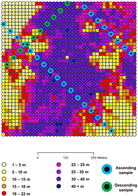
Figure 2. Near canopy top height (height from below which 96% of lidar energy returns) for GEDI footprints simulated from airborne data in one of six sites in the Pennsylvania/New Jersey study area. A possible sample of three clusters is shown.
Download figure:
Standard image High-resolution imageThe population parameter of interest is the average of the true AGBD over the N population elements (potential GEDI footprints), where N is the total number of population elements in a grid cell. For a 1 km grid cell, N is equal to 2500 20 × 20 m population elements, where the footprints in this realization would have a 20 m diameter. There is a parametric model, g(x, α), of AGBD in Mg ha−1, where x are characteristics of the GEDI waveform for the GEDI footprint, and α is a vector of parameters. The true AGBD for a footprint is assumed to deviate from the g(x, α) by a random quantity, ε, with an expected sum of zero. Under the assumption that the model is an unbiased predictor of the true AGBD, and ignoring model misspecification error, the modeled value g(x, α) will be used in place of the true AGBD. The mean can be expressed in terms of GEDI ground clusters. There are M non-overlapping clusters distributed across all possible tracks. There are Ti footprints in the ith cluster. The reader may have noted that each population element is in one ascending cluster and one descending cluster. We can express the population attribute, the average expected predicted AGBD over the N population elements, in terms of the clusters; that is:

where the modeled AGBD for each population element occurs in the numerator twice.
Equation (1) will be expressed in an equivalent form, for which there is an estimator and a method of calculating an approximate variance. Let  equal the cluster total of the predicted AGBD per hectare for the footprints in the ith cluster. Equation (1) can be expressed as the ratio of the mean (or sum of) AGBD per cluster and the mean (or sum of) number of elements per cluster:

Parameter estimates,  for the model g(x, α) are based on a separate sample, Sm, that is independent of the 1 km grid cell. In equations (1) and (2) the parameters, α, are replaced by the parameter estimates,
  and the population number of clusters, M, by the sample number of clusters, m, to get the estimator
  i.e. Gi with
The second component of the equation expresses the estimator  the sample mean of all predicted AGBD (per sample element) which is an estimator of the population average expected AGBD (per element). The population true average AGBD differs randomly from the expected value
  by the population average
  of the N deviations εit. For large N the contribution of
  to the total random error can be assumed negligible compared to the other two sources of uncertainty (the sampling error and the variability due to the model, see below), even if spatial autocorrelation is present. Hence, it is sufficient to assume the size of the grid cell (and thus N) is large enough to imply that the average
  will be close to zero. This assumption, along with the assumptions related to model fit will be covered in the discussion section.
As noted in the Introduction, the GEDI sample will be treated as a random sample of clusters of GEDI footprints. The estimator in equation (3) can be viewed as estimating the mean of cluster totals and mean number of footprints separately, and then combining as a ratio estimator:
This estimation strategy combines a probability sample of auxiliary information (as opposed to wall-to-wall auxiliary information) with a prediction for the population element value, AGBD, instead of directly observing AGBD. Ståhl et al (2011) proposed an estimator of the form of equation (4) and derived an estimator of the approximate variance. Due to the small sample size used in that study in relation to the population size, Ståhl et al (2011) did not include a finite population correction. A finite population correction may need to be taken into account in GEDI's case. Expression (5) below is the variance estimator proposed in Ståhl et al (2011), with the addition of the finite population correction:
The first term is due to the sampling error and the second term is due to effects of uncertainty of the  estimates (Ståhl et al 2011). The
  is the estimated covariance matrix of the p-parameter estimates, where the estimate is based on the separate set of data, Sm, that is independent of the 1 km grid cell. For simplicity the first term is referred as the sample component and second term the model component. If we assume a linear model, that is
  where xitj is the jth component of xit, then,
  Let
Let  be the vector of the means of the cluster totals of the predictor variables, i.e.
  for j = 1, ..., p. Then the second component on the right side of equation (5) can be expressed in matrix notation:
Note that  is equal to
  In the construction of equation (5), a Taylor linearization process is used twice; first with regards to the model parameters of
  (Ståhl et al 2011) and second to estimate variance of a ratio estimator (Särndal et al 1992).
The empirical data described in section 2.2 were used to calibrate the simulation study described in section 2.3 to evaluate the statistical properties of these estimators in the GEDI setting.
2.2. Supporting datasets
Lidar and field data collected over six diverse areas in the United States supported this study. These areas were defined by the non-overlapping window (Thiessen Scene Area) of a local Landsat scene. The six scenes (given by numeric WRS-2 Path/Row) included one each in: northern Maine ('ME': 12/28, excluding the Canadian portion); eastern Pennsylvania and central New Jersey ('PA/NJ': 14/32); coastal South Carolina ('SC': 16/37); northern Minnesota ('MN': 27/27); northwestern Colorado ('CO': 35/32); and western Oregon ('OR': 45/30) (figure 3). The selected areas represented a wide range of forest ecosystems and disturbance processes, as described by Cohen et al (2017) and Healey et al (2018). Small-footprint lidar was collected at each site in the pattern displayed in figure 3, and a waveform simulator developed by the GEDI Science Definition Team was used to simulate GEDI waveforms from the airborne data. Data collection and waveform simulation is described in appendix S1.
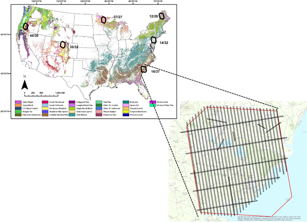
Figure 3. Location of the study's six focal areas, with detail for the SC site (24/34) showing airborne lidar flight lines. The width of each line was variable: ∼300–900 m. Adapted from Healey et al (2018).
Download figure:
Standard image High-resolution image2.3. Evaluating estimator performance
Simulations were conducted to examine the properties of the above estimators of mean AGBD and variance of the estimated mean. Modeled AGBD values treated as truth for each population element were developed for sixty square grid cells (ten randomly chosen grid cells at each of the six test areas in figure 3) of dimensions approximately similar to GEDI's product specifications. These populations were created by applying a linear model to the GEDI metrics simulated from actual small-footprint lidar acquisitions (figure 2). Appendix S2 details the process of both establishing the true population and simulating different potential cluster patterns and model parameter combinations to test the proposed estimators under a range of conditions. The advantage of using real data to develop the 'true' population, as opposed to simulating arbitrary AGBD surfaces, was that it ensured realistic covariance among lidar metrics. To the degree that lidar metrics are correlated with AGBD (see appendix S3), this approach also created a realistic spatial representation of biomass and of residual prediction error when different realizations of model parameters were applied to the lidar metrics. The swath width of the available lidar data limited the size of these test cells to between 680 × 680 m and 800 × 800 m (instead of 1 km); as mentioned earlier, this was considered adequate for the tests described below.
3. Results
The mean true AGBD of the 60 simulated grid cell-scale populations ranged from 1 to 183 Mg ha−1. There was little difference between the true and expected estimated values across simulated grid cells (figure 4). Divergence between these quantities centered around zero, and decreased with more clusters (figure 5).
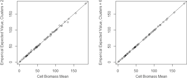
Figure 4. Expected estimate of AGBD (Mg ha−1) versus true AGBD (on the X axis) for both two and six tracks. The line represents y = x.
Download figure:
Standard image High-resolution image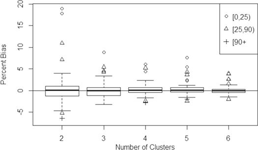
Figure 5. Boxplot of percent bias for ABGD estimates (equation (4)) at the grid cell level. Outliers are divided into categories defined by the mean AGBD for the simulated cell (0–25, 25–90, and 90 + Mg ha−1).
Download figure:
Standard image High-resolution imageThe empirical percent bias of the variance estimator (equation (5)) as a function of number of clusters is shown in figure 6. The estimator appears to be only asymptotically unbiased, with mean underestimation of variance at approximately 21% with two clusters and 2% with six clusters. Outliers in figures 5 and 6, which measure bias as a percent of the mean AGBD, tended to be low-biomass locations.

Figure 6. Boxplot of the empirical percent bias in the variance estimator for each grid cell (equation (5)). Outliers are divided into categories defined by the mean AGBD for the simulated cell (0–25, 25–90, and 90 + Mg ha−1).
Download figure:
Standard image High-resolution imageThe variance under-prediction at low numbers of clusters may be traced to the sample component of equation (5), not the model component (figure 7).
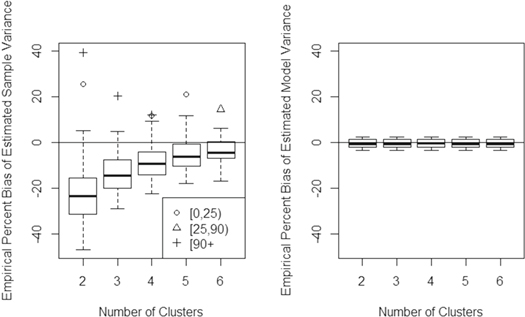
Figure 7. Decomposition of bias in overall grid cell-level variance estimates (figure 6) into sample and model contributions.
Download figure:
Standard image High-resolution imageIn most cases, the sampling component of the variance was larger than the model component (figure 8). With more tracks, overall variance of the estimate went down, and model variance accounted for a larger percentage of that variance.

Figure 8. Sample variance as a percentage of the total variance versus the percent standard error (square root of the variance) for 2 clusters and 6 clusters. More clusters reduced both overall variance and the importance of the sample component of the variance.
Download figure:
Standard image High-resolution image
4. Discussion
4.1. Advantages and assumptions
Earlier work with NASA's Geoscience Laser Altimeter System instrument pioneered the use of spaceborne lidar to make forest AGBD maps, often employing models that related field biomass to lidar and then, in a separate stage, related lidar-modeled biomass to synoptic data from sources like the MODIS satellites. While some work has attempted to impose a statistical framework on the use of such maps (e.g. Nelson et al 2017), most have employed ad hoc approaches to uncertainty. Mitchard et al (2014) pointed out two such ad hoc error budgeting approaches that yielded estimates across the Amazon that did not overlap with each other's relatively narrow confidence intervals, suggesting unacknowledged uncertainty in one or both estimates.
Saarela et al (2016) concluded that ignoring error occurring in the field-to-lidar step, as is often done, can lead to underestimation of variance by a factor of three. The spatial mismatch inherent in modeling AGBD in large pixels from constituent smaller-footprint measurements can also introduce uncertainties not clearly addressed in variance estimates (Réjou-Méchain et al 2014). The proposed hybrid approach does explicitly account for field-to-lidar model error, and it also accounts for sample error as footprints are combined to infer mean 1 km AGBD.
However, the hybrid approach summarized in figure 1 is subject to at least three important assumptions. The first is that the GEDI waveform simulator (Hancock et al 2019; described in appendix S2) correctly translates pulse counts to waveform data while representing the important sources of error. The benefit of using simulated GEDI data at precisely known locations to build footprint-level models is that it obviates potential error related to the positional uncertainty of GEDI footprints (currently estimated to be on the order of 10 m, post-processed). The risk is that any systematic simulator error may be propagated through footprint-level models to bias the 1 km mean AGBD estimates. However, the simulator is based on well-validated work by Hofton and Blair and Hofton (1999) and it is unlikely that violations of this assumption are substantial.
A second assumption is that one square kilometer is a large enough domain, given spatial autocorrelation of the population, that residual model error may be considered negligible. Mean residual error in the footprint AGBD model is presumed to tend toward zero over a large number of predictions. In an area that is small, particularly if spatial autocorrelation of residual error is high, residual errors may not sum to zero, introducing additional error. While GEDI's 1 km spatial domain is smaller than other applications of hybrid inference (e.g. Ståhl et al 2011), initial exploration using the data from this study suggests that spatial autocorrelation at GEDI's 25 m grain size is relatively low, as is the effect of omitting residual error (also called individual error in appendix 3) from the proposed hybrid variance estimator (appendix 3). In some cases, however, the impact of residual error may reach 15% or more of the variance, so further work is needed to develop ways to include it in the hybrid approach.
Finally, it is assumed that the footprint-level AGBD model is correctly specified and 'applies' to the population in the cell. This notion implies that the number and order of terms are correctly specified, and that the parameter covariance matrix used in the variance calculation (equations (5) and (6)) adequately reflects uncertainty in the relationship between lidar and AGBD within the cell. Since even small model difference can generate strongly divergent population estimates when multiplied over large areas, this is a critical assumption. Although the GEDI team is collating a comprehensive global database of training data, the reality is that ground data are sparse in some areas. In such areas, model misspecification is an important risk. In this respect, hybrid inference is no different from any other remote sensing approach that relies upon field data to calibrate remotely sensed observations.
4.2. Performance of hybrid estimators in the context of GEDI's sample
Properties of the hybrid estimators proposed for the GEDI mission were evaluated here using simulations in which thousands of potential GEDI cluster patterns were tested in the context of model covariance across forests in 60 diverse grid cells. Bearing in mind the above assumptions associated with the approach outlined in figures 1, 4 and 5 suggest that the proposed estimator for mean AGBD exhibits negligible bias across cells. Our tests and the results in figures 4 and 5 presumed proper model specification, an assumption of model-based inference, although residual plots (figure S4(1)) suggested that trends in model residual error may exist in at least one study region. In such cases, corrective measures such as variable transformations may be required.
The variance estimator, on the other hand, appeared to be only asymptotically unbiased (figure 6); that is, bias approached zero as larger numbers of cluster samples were acquired. The Taylor linearization used to compute the sample component of the variance (as opposed to the model component) likely contributed to this underestimation. While Taylor linearization simplifies calculation of the variance, it is known to lead to variance underestimation for small sample sizes (Särndal et al 1992, p 176). One area of future work may center around methods proposed to adjust for under-estimation (Cochran 1977, p 156). Linearization was also used in deriving the model component of the variance estimator (equation (5)), but the linear model used in this study for footprint-level prediction likely eliminated the impact of linearization in the model component.
Negative bias in the variance estimates at low numbers of clusters should be considered when hybrid methods are used with GEDI data, and information about the number of clusters will accompany GEDI hybrid estimates for each cell. Low sample numbers will occur both at the beginning of the mission and in equatorial regions where the ISS orbit provides fewer 'looks' and where persistent cloud cover may frequently obscure the surface. An advantage of hybrid estimation is that the same methodology applied at the 1 km scale may also be applied to much larger, irregularly shaped areas such as entire countries; instead of having to combine grid cell estimates, all clusters intersecting a given country may be used in the context of a single hybrid estimate. GEDI country-scale sample size will be very large, leading to greatly diminished design-based contribution to variance estimates. The apparent dominance of the sample component in the variance estimator (figure 8) may be relevant to GEDI operational planning. There are signal-to-noise parameters that may allow GEDI to consider a larger sample of noisier footprints (and models) or a smaller sample of footprints collected under ideal atmospheric conditions. It should be recognized that the relative contribution of the sampling and model components of the variance estimator may differ in different settings as properties of the model change due, for example, to the size of Sm or complexity of the underlying lidar/forest structure relationship. Across the diverse ecosystems we studied, though, results suggest that including a larger sample will have a bigger impact on the magnitude and unbiasedness of estimated variance than a marginal improvement in model fit.
5. Conclusions
The GEDI mission was conceived to support estimation of forest biomass at greater accuracy and resolution than has previously been possible by greatly increasing the number of available observations of forest structure. The sampling pattern employed by GEDI is largely constrained by its technology: its deployment platform on the ISS, the number and strength of its lasers, and its mission duration. Central to the GEDI approach has been the creation of a framework within these observational constraints for properly estimating both mean AGBD and the variance around that estimated mean.
Our research suggests that a hybrid approach that accounts for uncertainty due both to the model and the sampling design is appropriate and effective. Analysis here focused on 1 km cells, but hybrid inference using GEDI data could likewise be applied over any political or ecological units of interest, subject to minimum size and model applicability assumptions cited above. Our results confirm the importance of having abundant field plot estimates of biomass and associated airborne lidar, from which representative models that relate lidar metrics to AGBD may be created. The creation of a global database of such field and lidar data has been a priority of the GEDI mission before launch, and its continued expansion should both reduce the model uncertainty carried into 1 km variance estimates and support the local applicability assumptions that underlie model-based inference.
Lastly, our research also suggests that maximizing the number of clusters within a cell is key towards providing approximately unbiased variance estimates. While observational strategies to increase cluster density are limited, options such as purposefully targeting important areas, lengthening mission duration, or increasing the size of grid cells to encompass more clusters are worth exploring.
Acknowledgments
This work was supported by grants NNH13AW62I and 80HQTR18T0016 from NASA's Carbon Monitoring System (solicitation NNH16ZDA001N) as well as support from the NASA GEDI Science Definition Team. The authors appreciatively acknowledge constructive input from three anonymous reviewers.