

Abstract
Variables describing the abiotic environment (e.g. climate, topography or biogeographic history) have a long tradition of use as predictors of tree species richness patterns. However, these variables may capture variations in richness related to climate, but not those that are related to soil type or forest disturbance. Canopy structure has previously been shown to provide information on the variation of tree species richness, with richness generally increasing with larger canopy heights and denser foliage. The use of canopy structure is increasingly relevant with the availability of such data from the Global Ecosystem Dynamics Investigation (GEDI), a lidar mission onboard the International Space Station. In this analysis we show that GEDI canopy structure explains up to 66% of the variation in tree species richness in natural forests without a history of recent disturbance across the globe. However, this portion overlaps with the variation (up to 80%) explained by environmental and biogeographical variables. Our results show that relationships between tree species richness on one side and climate and canopy structure on the other side are not as straightforward as we initially expected, and should be further investigated across both natural and disturbed forests.
Export citation and abstract BibTeX RIS

Original content from this work may be used under the terms of the Creative Commons Attribution 4.0 license. Any further distribution of this work must maintain attribution to the author(s) and the title of the work, journal citation and DOI.
1. Introduction
Tree species diversity varies greatly across the Earth, ranging from about one species per hectare in boreal forests at high latitudes, to several hundred species per hectare in tropical forests (Keil and Chase 2019). Understanding and predicting this variation is important because tree diversity has been linked to ecosystem services, such as productivity and carbon accumulation (Huang et al 2018, Craven et al 2020), and accurate predictions of diversity can improve future conservation decisions (Algar et al 2009).
Because of logistical and taxonomic challenges, it has so far been impossible to measure tree diversity directly in the field over large, continuous areas. Instead, we only have information from discrete, isolated forest plots (Šímová et al 2011, Ricklefs and He 2016, Sullivan et al 2017, Keil and Chase 2019). A common practice is to link diversity in these plots to environmental predictors (e.g. climate, topography, land cover, and other spatial predictors) using parametric statistical models or machine learning algorithms (e.g. Ricklefs and He 2016, Keil and Chase 2019, Večeřa et al 2019). These can then be used to predict diversity to unsurveyed areas, and to test hypotheses about the role of various predictors driving variation in diversity. Thus far, climatic variables describing the water-energy balance (such as evapotranspiration, precipitation, temperature, remotely sensed proxies of productivity, and their seasonality) have been particularly effective predictors of local plant and tree diversity over large geographic extent, explaining considerable fractions of variation (see table 1 for examples). However, there is still a margin of improvement, for example, climatic, topographic, and land-use variables only explain a small portion of the variation in richness in some regions (e.g. continental US; Craven et al 2020).
Table 1. Several examples of studies modelling the relationship between tree diversity in local samples (plots) and environmental predictors, and the percentage of variation in species richness that the models were able to explain.
| Reference | Geographic extent | Spatial grain | Predictors | Modelling method | Explained variation |
|---|---|---|---|---|---|
| Craven et al (2020) | USA | 0.0672 ha, FIA plots | Productivity, topography, climate, land use, area | Random forest | 37% |
| Keil and Chase (2019) | Global | Varying | Climate, topography, space, productivity, area | GAM | 88% |
| Ricklefs and He (2016) | Global | Varying, CTFS plots | Climate, space, # of trees | GLM | 92% |
| Šímová et al (2011) | Global | 0.1 ha, Gentry plots | Climate, space | GLM | 76% |
| Francis and Currie (1998) | Northern temperate zone | Varying | Climate, area, space | LM | 76.5% |
| Kay et al (1997) | South America | Local plots (unclear) | Climate (rainfall) | Local regression | 65% |
| Ganzhorn et al (1997) | Madagascar | 0.1 ha | Climate (rainfall) | Correlation | 50% |
| Specht and Specht (1994) | Australia | 1 ha | Productivity | LM | 98% |
| Clinebell et al (1995) | Northern Neotropics | 0.1 ha, Gentry plots | Climate, soils | LM | 53% |
One way to potentially improve the existing models of tree diversity is through the use of forest structure. Canopy structure depends on environmental factors, soil, disturbance and crown plasticity (Frolking et al 2009, Jucker et al 2015, Pfeifer et al 2018, Senf et al 2020, Hakkenberg and Goetz 2021) and thus may contain information on tree species diversity that cannot be captured by environmental variables alone. There are theoretical reasons that may explain why forest structure (such as height, total volume, or complexity of canopy) should predict richness. First, due to sampling effects (Šímová et al 2011), a more diverse forest could have sampled species (from regional species pool) that fill the upper canopy, as well as shade-tolerant species in the forest understory. Second, canopy height can be considered a proxy for canopy volume, which may correlate with the volume of niche-based opportunities for species to coexist. Both effects can increase diversity in more complex, higher, and voluminous canopy structures, through niche complementarity and resource partitioning (Schoener 1974, Chase and Leibold 2003) and there is empirical evidence that forests with higher canopies have a higher plant species diversity (Gatti et al 2017). Furthermore, studies using vertical canopy structure data derived from full-waveform lidar explained more of the variation in tropical tree species richness than canopy height alone (Marselis et al 2019, 2020). Such models become increasingly relevant with the availability of more detailed information on not only canopy height, but also the density of canopy material along the vertical forest axis. The Global Ecosystem Dynamics Investigation (GEDI) mission (Dubayah et al 2020), launched in December 2018, is now providing a large set (billions) of such canopy structure measurements. However, the potential of canopy structure, such as observed by GEDI, to predict broad-scale patterns of tree biodiversity remains unknown.
Here we evaluate the efficacy of the GEDI-derived canopy structure to explain variation in tree species richness in natural and semi-natural forest plots at a near-global extent covering both the tropical and temperate regions. We also compare the efficacy of canopy structure variables within predictive models of tree species richness with other previously used predictors, namely those related to climate, topography, and biogeographic history, as used in Keil and Chase (2019).
2. Methods
2.1. Data
We used tree species richness data which were compiled from publicly available, previously published studies, by Keil and Chase (2019). Specifically, the dataset consisted of data on species richness from 1166 forest plots in tropical and temperate regions from across the world. These forest plots were originally selected by Keil and Chase (2019) to represent both temperate and tropical natural and semi-natural forests across as many biomes and biogeographic realms as possible given open access data availability. Nevertheless, as with most such analyses, there are considerable data gaps in large parts of Africa and Asia due to limited availability of forest plots from these regions. Only plots from natural or semi-natural forest (e.g. not from plantations, production forests, or severely disturbed/damaged forests, for example, as a result of logging, hurricanes, or bark beetle outbreaks) were used. These plots were taken from published database compilations (Phillips and Miller 2002, Phillips et al 2003, Ramesh et al 2010, Anderson-Teixeira et al 2015, Coelho de Souza et al 2016, Ricklefs and He 2016, Sullivan et al 2017), national forest inventory surveys (De Natale et al 2005, USDA 2016, IGN 2017), and extracted manually from primary sources (Beals 1965, Yamada 1976, Abbott 1984, Kohyama 1986, Cao and Zhang 1997, Linder et al 1997, Ansley and Battles 1998, Narayanan and Parthasarathy 1999, Maycock et al 2000, Adam 2001, Kohira et al 2001, Cairns et al 2003, Enoki 2003, Hirayama and Sakimoto 2003, Cheng-Yang et al 2004, Fashing et al 2004, Jing-Yun et al 2004, Sheil and Salim 2004, Shu-Qing et al 2004, Wu et al 2004, Bonino and Araujo 2005, Davis et al 2005, Sawada et al 2005, Splechtna et al 2005, Adekunle 2006, Graham 2006, Malizia and Grau 2006, Szwagrzyk and Gazda 2007, Lopes et al 2008, Yasuoka 2008, Addo-Fordjour et al 2009, Eichhorn 2010, Krishnamurthy et al 2010, Lalfakawma et al 2010, Nagel et al 2010, Namikawa et al 2010, Lü et al 2010, Eshete et al 2011, Round et al 2011, Sanchez et al 2013, Popradit et al 2015, van Do et al 2015, Wusheng et al 2015). For each plot we used the number of tree species (S) as our focal response variable. From the abovementioned studies we further extracted three covariates related to sampling design, which can all influence the observed S, and thus need to be controlled for in statistical analyses. These covariates were:
- The total area of the sampled plot (km2).
- The minimum diameter at breast height (minDBH in cm); only trees of equal or larger diameter than minDBH were measured and included in the analysis.
- The number of trees larger than the minDBH in the sampled plot.
For each plot, we considered six variables related to the climate, topography, and biogeographic history which were previously successfully used to explain tree species richness in Keil and Chase (2019). These were:
- WorldClim (Hijmans et al 2005) mean annual temperature (BIO1), mean isothermality (BIO3), and mean precipitation seasonality (BIO15), which are 1970–2000 spatially interpolated averages extracted from rasters with a resolution of 30 arc-seconds (1 km2 around equator) available at www.worldclim.org/data/v1.4/worldclim14.html.
- Absolute difference between the lowest and highest elevation in a 30 arc-seconds raster cell within which a given plot is located, derived from Danielson and Gesch (2011).
- Island vs. mainland, a binary factor indicating if a plot is on an island or mainland (from Weigelt et al 2013), following a loose classification in which shelf islands (connected to mainland in the past) are classified as islands.
- Classification of biogeographic realms into Afrotropic, Australasian, Easter Palearctic, Indo-Malay, Nearctic, Neotropic, and Western Palearctic, following (Ricklefs and He 2016).
For further details on these environmental data, see supplementary material of Keil and Chase (2019).
We used GEDI-derived variables describing canopy structure from the first two years of data collection: April 18, 2019–May 14, 2021. GEDI is a sampling instrument mounted to the International Space Station, collecting lidar data between 51.6° N and S. GEDI has three lasers that are split into four beams total. The beams are dithered across track, resulting in eight beams along-track. The footprint-spacing along track is 60 m and the across-track spacing is 600 m. At each sampling location, GEDI collects a full-waveform with a nominal footprint size of ∼25 m (Dubayah et al 2020). During the first two years of the mission, GEDI was programmed to collect data with the least spatial overlap, acquiring the densest possible sampling at the footprint level. Because of the sampling method, footprints do not necessarily overlap exactly with the sampled forest plots from Keil and Chase (2019), thus we used the information from GEDI footprints in square buffer zones around the original plot locations. This also ensures that we capture the canopy structure of the forest plots for those plots with a limited spatial location accuracy. GEDI footprints themselves have a geolocation accuracy of about 10 m. We included plots that have at least one GEDI footprint within the buffer zone around the plot centre. We evaluated three buffer zones (figure 1(b)):
- 1 × 1 km buffer zone (1 km2, 888 plots).
- 2 × 2 km buffer zone (4 km2, 978 plots).
- 4 × 4 km buffer zone (16 km2, 1053 plots).
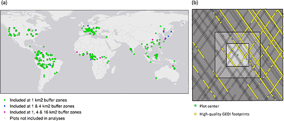
Figure 1. (a) Locations of the original 1166 forest plots; the number of plots included in the analysis was lower as not all forest plots were close to GEDI footprints. Colored markers indicate for which buffer zone the plots were included. (b) Example of a forest plot from Coelho de Souza et al (2016), plot JEN-13 in the Amazon. Plot centre indicated with green marker, three concentric squares indicate buffer zones for the 1, 4, and 16 km2, GEDI footprints are indicated with yellow (high quality data, used) and open markers (insufficient quality, unused). For each buffer zone all high quality GEDI footprints within that buffer zone are used in the analysis; e.g. the footprints within the 1 km2 are also included in the 16 km2 zone.
Download figure:
Standard image High-resolution imageThere were some plots where no GEDI shots intersected any of the buffers because of its sampling method. Moreover, the number of plots available at the different buffer zones increases with the size of the buffer zone (varying from 888 to 1053 plots out of the original 1166 plots considered, figure 1(a)).
According to Marselis et al (2019, 2020), the most important GEDI metrics related to tree species richness were: canopy height, total plant area index and the plant area index along the vertical forest axis divided into 10 m vertical bins. We adopted this same set of metrics. However, to confirm that other canopy structure variables do not explain more of the variation in richness, we included the results of a principal component analysis (PCA) analysis performed on a large set of canopy structure metrics (180 metrics, appendix
- Canopy Height, measured as the relative height at which 98% of the energy was returned (RH98).
- Total plant area index (PAI) along the vertical forest axis
- The total PAI between 0 and 10 m vertically, m2/10 m3
- The total PAI between 10 and 20 m vertically, units in m2/10 m3
- The total PAI between 20 and 30 m vertically, units in m2/10 m3
- The total PAI between 30 and 40 m vertically, units in m2/10 m3
- The total PAI between 40 and 50 m vertically, units in m2/10 m3
- The total PAI above 50 m vertically, units in m2/10 m3
- The ground elevation
All these metrics were derived from the GEDI Level 2A and 2B datasets version 2 (Dubayah et al 2021a, 2021b). The L2A GEDI dataset contains the relative height (RH) products of the processed, geolocated waveform, including RH98 (essentially canopy height) and the ground elevation. The L2B dataset contains the vertical profile metrics; including the total PAI and the PAI along the vertical axis. GEDI L2A data contains information from four processing algorithms applied to the geolocated waveforms. We used the canopy height and ground elevation from the processing algorithm flagged as the 'best' algorithm for each shot in the GEDI dataset (Dubayah et al 2021a, 2021b). We also only included waveforms that were collected in the leaf on season, using the 'leaf off flag' in the GEDI data products. Lastly, only waveforms that were flagged '1' for the metric 'successful processing at the 2b data level' (vertical canopy structure, Dubayah et al 2021b) were considered reliable and used in this analysis.
For each of the 16 km2, 4 km2 and 1 km2 areas, we calculated the average of the nine canopy structure metrics from all footprints within the buffer zone and joined them to the field and environmental data, creating three final datasets (one for each buffer zone).
2.2. Analysis
2.2.1. Raw relationships
In a first exploration, we examined the general relation between the observed tree species richness and canopy structure using just two selected canopy structure metrics, canopy height and total PAI, as these are descriptors of the general canopy structure and have previously shown significant relationships with tree species richness in the tropics (Marselis et al 2020). This preliminary analysis gives insight in variation in the used data, and it shows naïve relationships when failing to control for the effects of other variables.
First, to show the relationships in the raw data, we fitted single-term generalized linear models, with S as a response (quasi-Poisson errors, log link function) and canopy height or total PAI as predictors. We performed a second exploratory step as S can be affected by sampling protocols that vary among plots. Thus, we examined these relationships after controlling for the effects of covariates related to sampling protocol. To do this, we first fitted a 'covariate' random forest (RF) model (see below in the variation partitioning section), with plot area, number of tree individuals, and minDBH as predictors of S. We calculated the residuals as (observed log10 S) − (predicted log10 S), and fitted a generalized linear model (normal errors, identity link function) to these residuals as a function of canopy height and total PAI. We chose this model because, unlike the raw counts of species (S), residuals centre around 0 and thus cannot be modelled by the distributions designed to model count data (e.g. Poisson, or quasi-Poisson).
2.2.2. RFs
We used RFs (Breiman 2001) as the main analytical tool to evaluate the relationships between the main response variable tree species richness (S) and all the other predictors. Specifically, we used RF setting with 1000 trees and the default settings of the 'randomForest' function implemented in R package (randomForest v 4.6–14), to model S as a function of study design covariates, and environmental, biogeographical, and GEDI-derived predictors (details are below).
2.2.3. Collinearity and variation partitioning
Our data are observational and can potentially suffer from collinearity problems. Specifically, forests in tropical warm and humid areas may have similar canopy structures, which are different from forests in other biomes (e.g. cold and/or dry climates). This means that species diversity can potentially be explained either by environmental predictors (precipitation, temperature, primary productivity, topography, biogeographical history), or by GEDI canopy structure, and we may potentially have no way to tease these two apart. We show the relation among predictors in appendix
To do the variation partitioning, we fitted four separate random forests:
- (a)RFcov with covariates describing size of the plot, number of trees and minDBH, but no environmental or GEDI predictors.
- (b)RFenvi_only with covariates and environmental predictors.
- (c)RFGEDI_only with covariates and GEDI predictors.
- (d)RFfull with covariates, environmental predictors, and GEDI predictors.
We measured the amounts of variation in S explained by these random forests using Rcov, Renvi_only, RGEDI_only and Rfull respectively, where each of these is a coefficient of determination (R2) from the respective RF model. We thus get Renvi_only = Rfull − RGEDI , RGEDI_only = Rfull − Renvi, and Rshared = Rfull −(RGEDI_only + Renvi_only). We did the RFs for each of the three buffer zones, resulting in 12 global RFs. The data and code are at: https://figshare.com/s/82d033d5592889af48bc (Marselis and Keil 2022).
3. Results
Examination of the raw relationships (using a 16 km2 buffer zone) revealed a significant positive relationship between the number of tree species with both canopy height and total PAI (figure 2). This relationship was significant in the raw data (figures 2(a) and (b)), and also after accounting for the effects of study design covariates: plot area, total number of individuals, and minimum DBH (figures 2(c) and (d)). However, the relationships were weaker in the residuals than in the raw values, and there was a substantial fraction of variation around the fitted lines (figure 2).
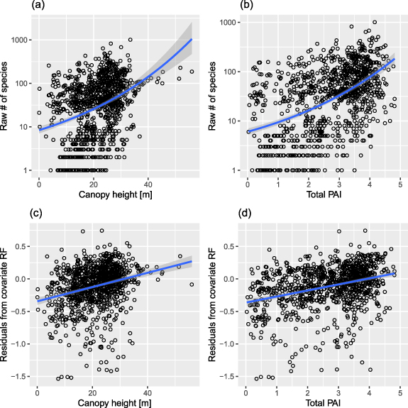
Figure 2. Bivariate relationships between number of species (species richness, S) in forest plots and two GEDI-derived variables: canopy height (a), (c) and total Plant Area Index—PAI (b) and (d). In the top row (a) and (b) are raw species numbers as reported in each study, and a quasi-Poisson regression (log link function). In the bottom row (c) and (d) we show residuals of a random forest model accounting for plot area, number of tree individuals, and minimum diameter at breast height. To calculate the residuals, we log10-transformed the observed and predicted values of S. A linear regression (normal errors) was then fitted to the residuals. All relationships are statistically significant (with P < 0.001). Grey bands show standard errors.
Download figure:
Standard image High-resolution imageThe observed vs. predicted plots for the four RF models show that both environmental and GEDI predictors explain substantial fractions of variation in tree species richness at the 16 km2 buffer zone (figure 3), although the environmental predictors alone explain more than the GEDI predictors alone (figure 4). Specifically, 80% of the variation in tree species richness was explained by the covariates and environmental variables (Renvi, figure 4(a)). GEDI variables, in combination with the covariates, explained 59% of this variation (RGEDI, figure 4(a)). A random forest model that used both GEDI canopy structure and environmental variables explained just 77% of the variation (Rfull, figure 4(d)). Importantly, the fraction of variation explained by GEDI overlaps with the fraction explained by the environmental variables (figure 4(a)). For partial dependence plots of the RF models, see appendix

Figure 3. Observed versus predicted plots of the response variable of the random forest (RF) models with the 16 km2 buffer zone for the four models. Diagonal line shows the perfect 1:1 match.
Download figure:
Standard image High-resolution image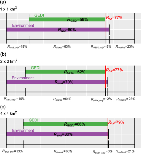
Figure 4. Variance of tree species richness explained by the GEDI variables (green, model 3), the environmental predictors (purple, model 2), and the full model with both GEDI and environmental predictors (red vertical line, model 4). Panels (a)–(c) show results from RF models using GEDI variables from 1 km2, 4 km2, and 16 km2 buffer zones respectively. At the 16 km2 buffer zone (c): GEDI canopy structure alone explains 66% of variation in tree species richness, 80% of the variation can be explained with environmental variables alone. The full model, combining all variables, explains slightly less (negative percentage on x-axis) of the variation: 79% (red line, panel c); hence resulting in 21% unexplained variation.
Download figure:
Standard image High-resolution imageThe results for the models developed for the 4 and 16 km2 buffer zones were similar to those at 1 km2 zone. GEDI variables alone explained respectively 62% and 66% of the variation, the environmental variables 79% and 80% and the full models 77% and 79% (figures 4(b) and (c)). The fraction of variation explained by GEDI overlapped with the fraction explained by the environmental variables for both buffer zones.
4. Discussion
4.1. GEDI vs. environmental variables
The most important result is that, in local forest plots at a global extent, we were unable to unequivocally attribute variation in species diversity to GEDI-derived forest structure, nor to other environmental predictors. More specifically, even though forest structure (together with covariates describing study design) explained up to 66% of variation in tree species diversity, environmental predictors related to climate, topography, and history can explain even more variation in diversity (up to 80%), and there is no increase in explained variation when GEDI and environmental predictors are used together in one model. This means that GEDI-derived forest structure can indeed be used to explain local tree species diversity, which is in line with the relationship between canopy height and tree species diversity found by Gatti et al (2017), and it underpins the hypothesis that canopy structure data may serve to predict variation in tree species richness (Marselis et al 2020). However, if other environmental predictors are available they may provide even better diversity estimates than the GEDI-derived variables, and we found no clear advantage in combining the strengths of the two groups of predictors for the datasets we examined.
Even though this is a negative result from a practical point of view–the GEDI-derived forest structure does not improve existing correlative near-global models of tree species diversity–there is a valuable conceptual inference. Independent effects of forest structure and environment on forest diversity (figure 5(a)) are unlikely, because otherwise, including forest structure should have unequivocally improved the overall models. Our results are more consistent with an alternative (causal) pathway in which the abiotic environment drives both forest structure and species diversity (figure 5(b)); with the possibility of a secondary effect of forest structure on species diversity (figure 5(c)) or the possibility of a two-way effect where tree species richness also drives forest structure itself (figure 5(d)). However, our correlative models cannot reject or confirm this secondary link, since the overlapping fraction of explained variation (figure 4) is too large. Thus, we conclude that the three pathways (figures 5(b)–(d)) are all plausible. This is in line with other studies (Frolking et al 2009, Pfeifer et al 2018, Senf et al 2020, Hakkenberg and Goetz 2021) which hypothesize that canopy structure should depend on environmental factors, soil and disturbance. Potential evidence for the secondary effect (figure 5(c)) was found by Hakkenberg and Goetz (2021) who studied the relation between canopy structure, climate and tree species richness in forests of the United States. Their study showed that a small portion of the remaining variance was explained by climate x structure interaction terms. Such a result could not be reproduced at this global scale using GEDI canopy structure, potentially due to the differences in canopy structure metrics available as Hakkenberg and Goetz (2021) used high resolution discrete return airborne lidar data at 20 × 20 m plot level, which points to the importance of spatial scale, discussed below.
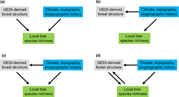
Figure 5. Four alternative causal pathways between environmental variables (blue), GEDI-derived forest structure (grey) and local tree species richness (green). Our results are consistent with panels (b), (c) or (d).
Download figure:
Standard image High-resolution image4.2. Limitations
Our tree species richness dataset only included data on natural or semi-natural forests; there were no (severely) disturbed forests, orchards, production forests, or plantations/monocultures. Thus, our forest plots mostly have a compact and well-developed canopy, which potentially reduces the variation of forest structure across the dataset, limiting the scope for the GEDI-derived structure to explain diversity. In contrast, human-affected forests have distinctly 'unnatural', regular, or loose canopies (Tropek et al 2014). If such forests were also included in the analysis, we might expect that the GEDI-derived forest structure should explain more variation in richness, and could even outperform the other environmental predictors. Here we see a potential for joint use of environment and GEDI-derived variables to predictions of actual richness of all forests, including those modified by humans, as opposed to potential richness of natural plots as in this study and in Keil and Chase (2019).
Furthermore, GEDI footprints are not randomly distributed in our plots' buffer zones and they may not exactly overlap with the plots. For example, GEDI measurements may only cover a part of the buffer zone (e.g. figure 1(b)). More local, plot-specific forest structure information could provide additional/different information on the canopy structure than our buffered and spatially averaged metrics, but unfortunately the GEDI sampling density is not high enough to assert this. Encouragingly, however, we did not find considerable differences in model performance between the smallest buffer zone areas (1 km2 and 4 km2) and a small improvement with the largest buffer zone area (16 km2). This is likely because structural variables derived from these different buffer areas are similar (appendix
The temporal mismatches between collection of the field data, the environmental data, and the canopy structure data should also be kept in mind. Forest growth and (small) natural disturbances alter the forest over the shorter and longer term (Senf et al 2020), resulting in a mismatch of the forest structure and representation of the tree species diversity. This is a limitation that is difficult to overcome because of the time-consuming and expensive field data collection. Here we assume that the data used here (with the GEDI data from 2019 to 2021, climatic data from 1970 to 2000, and forest plot data collected between 1962 and 2016) represent the long-term situation in these natural and semi-natural forests. We assume that changes of climate and species temporal turnover in these forests are slow enough to still allow a correlative analysis involving the more recent GEDI data. The high explanatory power of both the climate and GEDI-derived variables support this assumption, although the real consequences of this temporal mismatch are unknown and should be investigated in the future. Additionally, it is yet unknown how the temporal dynamics of GEDI observations acquired from different times within the same leaf-on season, as well as across leaf-on seasons, may affect our results.
4.3. Future research
Future research should further explore the more realistic hypotheses (i.e. figures 5(b)–(d). We need to step back to properly examine the relationship between abiotic conditions and forest structure (such as recently performed in the US by Hakkenberg and Goetz (2021)). Now that the GEDI data are available, a global analysis of this relationship using its massive amount of remotely sensed structure data is possible. This should enable us to further untangle the (causal) relationships between climate, forest structure, and disturbance, improve our understanding of ecosystem functioning, and enable the analysis of the real usefulness of canopy structure for mapping tree species richness in both natural and disturbed forests.
This also points to the importance of spatial scale in general. The question of the role of structure vs. environment in driving patterns of tree species richness should be explored as a function of scale. This could, for example, help to determine whether there are characteristic scales of analysis where structure dominates beyond environmental variables or vice versa. Such an analysis would require high quality species richness data (e.g. at 25 m2), across a landscape, along with vertical canopy structure data at the same resolution in spatially continuous grids. Answering this question is exceptionally difficult because these kinds of continuous field data are rare. Furthermore, it has been shown that grain of disturbances is spatially very small, with mean disturbance sizes of 10–20 ha across continents, but with a median strongly skewed towards smaller patches (∼0.1 ha) (Taubert et al 2018), and not inconsistent with the decorrelation of structure over hundreds of meters noted above. Given the importance of small-scale disturbance to tree diversity, this suggests the need for fine-grained information on canopy structure at global scales. GEDI provides the basis for obtaining such observations when used in combination with other continuous remote sensing data at fine (30–100 m) resolutions, such as may be obtained from passive optical sensors (e.g. Landsat; Potapov et al 2021) or from radar sensors that measure 3D structure (e.g. TanDEM-X; Qi et al 2019). GEDI data can provide the basis for machine learning and other fusion methods that predict not only height and biomass at fine scales, but potentially the imputation of entire waveforms, opening the door to pervasive canopy structure predictions, at fine scales, across the landscape.
Some of the complex interactions can perhaps also be teased apart by focusing on fully mapped forest plots such as those in the CTFS/ForestGeo network (Anderson-Teixeira et al 2015), which offer rich data on exact location and growth form of every individual tree, collected over multiple time periods, with growth form and species of each known individual. If these were connected with remotely sensed forest structure using fusion with GEDI, an analysis teasing apart the interplay between forest structure, diversity, and abiotic conditions across a variety of scales may be possible.
Lastly, alternative analytical approaches that accommodate complex causal pathways, for example, structural equation modelling (Iriondo et al 2003, Lam and Maguire 2012), can be adopted. A similar analysis has been done to evaluate the direct and indirect effects of forest taxonomical and structural diversity, soil fertility and climate on aboveground carbon storage in neotropical forests (Poorter et al 2015).
5. Conclusion
Overall, our analysis showed a significant relationship between canopy structure and tree species diversity for natural and semi-natural forest undisturbed forests. However, we found that GEDI canopy structure cannot be unequivocally linked to the variation in tree species richness in natural undisturbed forests because the portion of the variance explained by GEDI-derived canopy structure overlapped with the variance explained by environmental and biogeographical variables. Hence, to estimate tree species richness across broad spatial scales, GEDI-derived data, while useful, do not appear to provide any additional information for natural forests. Nevertheless, GEDI predictors may still be useful for explaining tree species richness in more disturbed forests that were not part of the current analyses, because environmental variables are less likely to contain information on changes in tree species richness that are linked to disturbance, and across fine spatial scales. Future research should include information on such disturbance gradients and further investigate the relationship between climate, forest canopy structure and tree species richness.
Acknowledgments
This work is supported by NASA contract #NNL 15AA03C to the University of Maryland for the development and execution of the GEDI mission (Principal Investigator, R Dubayah). J M C gratefully acknowledges the support of iDiv funded by the German Research Foundation (DFG—FZT 118, 202548816). P K was supported by REES (Research Excellence in Environmental Sciences) grant from Faculty of Environmental Sciences, Czech University of Life Sciences in Prague. The authors gratefully thank Dr. John Armston for assistance with the GEDI data and other useful inputs.
Data availability statement
The data that support the findings of this study are openly available at the following URL/DOI: https://figshare.com/s/82d033d5592889af48bc.
Funding
NASA: NNL 15AA03C
German Research Foundation: DFG—FZT 118, 202548816
REES (Research Excellence in Environmental Sciences) grant, from Faculty of Environmental Sciences, Czech University of Life Sciences in Prague.
Appendix A.: Principal Component Analysis on GEDI data
A PCA was performed to ensure that the chosen GEDI metrics (Marselis et al 2019, 2020) contained all information on canopy structure necessary to generate the structure-richness models. For this analysis the following set of GEDI metrics was extracted from all GEDI footprints and calculated at the 1 km2, 4 km2, and 16 km2, buffer zones:
- Mean elevation lowest mode (ground elevation)
- Foliage height diversity (FHD)
- Canopy cover
- Total plant area index
- Relative height at 0, 25, 50, 75 and 98% (RH0, RH25, RH50, RH75, RH98)
- PAI at 5 m vertical intervals
- Cumulative PAI at 5 m vertical intervals
For each of the buffer zones we calculated the mean, standard deviation, maximum and minimum of all footprints falling within the buffer zone. This resulted in a total of 159 metrics. The results show (table A1) that the model performance is worse at all buffer zones than when using the carefully selected canopy structure metrics based on their biophysical meaning (Marselis et al 2019, 2020).
Table A1. R2 of random forests built on GEDI metrics (GEDI), 5 (PCA 5), 10 (PCA 10) and 15 (PCA 15) principal components calculated from 159 GEDI metrics.
| Buffer zone | GEDI | PCA 5 | PCA 10 | PCA 15 |
|---|---|---|---|---|
| 1 km2 | 0.60 | 0.51 | 0.52 | 0.53 |
| 4 km2 | 0.62 | 0.53 | 0.54 | 0.55 |
| 16 km2 | 0.66 | 0.53 | 0.54 | 0.55 |
Appendix B.: Collinearity between GEDI and environmental variables
Plant Area Indices at the various height layers tend to strongly correlate to the previous height layer as usually the amount of plant material higher in the canopy depends on the amount of plant material lower in the canopy (figure B1).
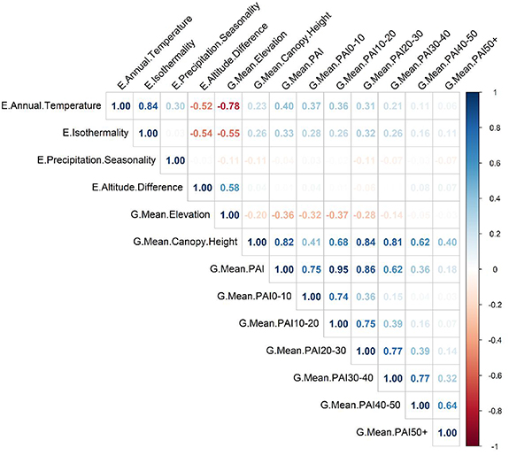
Figure B1. Correlation between the numeric environmental variables (starting with E.) and the GEDI canopy structure metrics (starting with G).
Download figure:
Standard image High-resolution imageAppendix C.: Relation of GEDI canopy metrics at different buffer zones
We included various buffer zones because of two main reasons: (a) it is not known what size buffer zone provides the most accurate modelling results and (b) the number of included plots would be higher with a larger buffer zone. The results show no real difference in model performance using canopy structure from the 1, 4 and 16 km2 buffer zones. The estimates of canopy structure from the buffer zones are unbiased (figure C1). The canopy structure at the exact plot location may differ from the canopy structure in the buffer zones, however, the canopy structure at the 16 km2 buffer zone is not biased, or in other words it does not describe a different canopy than the smaller buffer zones. This means that the canopy structure in each of the buffer zones could be regarded as the general forest structure at the plot location but does not necessarily constitute the small-scale variation in canopy structure at the plot location.
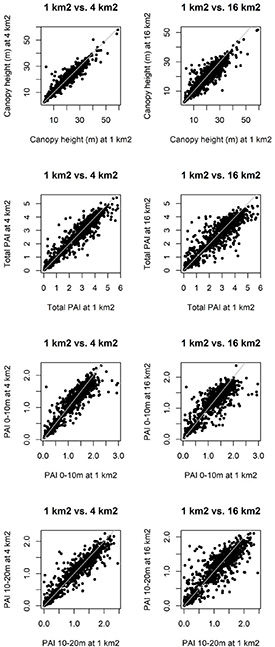
Figure C1. Relation between canopy structure metrics of GEDI at the 1 km2 vs. 4 km2 buffer zones and the 1 km2 vs. 16 km2 buffer zones.
Download figure:
Standard image High-resolution imageThe heterogeneity of the various canopy structure measurements does increase with buffer zone (table C1), this can be explained by the larger sample area (area of the buffer zone), describing a larger piece of forest, this is to be expected given that forest structure decorrelates within just a couple hundreds of meters (Réjou-Méchain et al 2014).
Table C1. The heterogeneity of the canopy structure slightly increases with buffer zones size. The table indicates for four important canopy structure variables the average standard deviation of e.g. canopy height for all plots at that specific buffer zone. This value is computed as the average of all buffer zones, using the standard deviation of all GEDI footprints within a buffer zone for the specified metric.
| 1 km2 | 4 km2 | 16 km2 | |
|---|---|---|---|
| Canopy height (m) | 7.00 | 7.55 | 8.14 |
| Total PAI | 1.30 | 1.37 | 1.42 |
| PAI between 0 and 10 m | 0.75 | 0.78 | 0.80 |
| PAI between 10 and 20 m | 0.60 | 0.63 | 0.65 |
Appendix D.: Partial dependence plots
The partial dependence plots show the response of species richness to a given predictor, after accounting for effects of other predictors and covariates (figure D1: GEDI predictors, figure D2: Environmental predictors). For example, mean total PAI has a positive relationship with species richness.
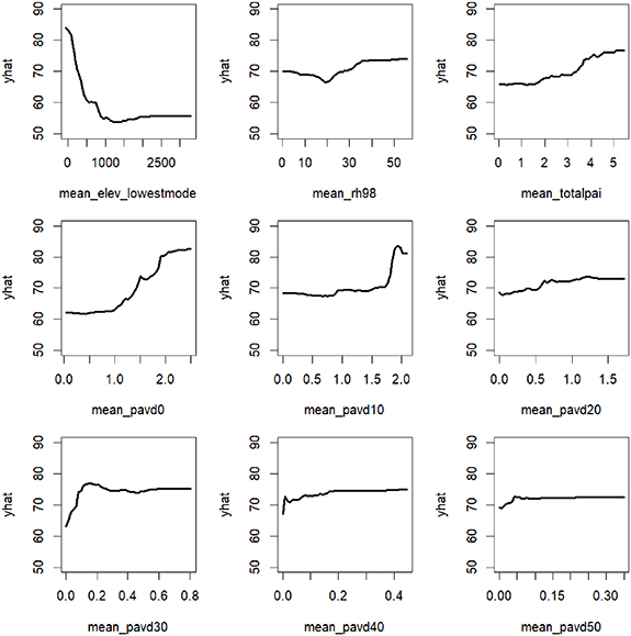
Figure D1. Partial dependence plots for random forest with covariates and GEDI predictors only (derived at 4 × 4 km buffer zone around each forest plot). Yhat is the response of species richness to a given predictor, after accounting for effects of other predictors and covariates. Abbreviations: mean_elev_lowestmode is the ground elevation, mean_rh98m is Canopy Height (RH98), mean_totalpai is Total Plant Area Index (PAI), mean_pavd0—mean_pavd50 is the total PAI at 10 m vertical intervals, with pavd0 meaning total PAI between 0–10 m vertically, pavd10 referring to total PAI between 10–20 m, etc.
Download figure:
Standard image High-resolution image
Figure D2. Partial dependence plots for random forest with covariates and environmental predictors only (derived at 4 × 4 km buffer zone around each forest plot). Yhat is the response of species richness to a given predictor, after accounting for effects of other predictors and covariates. Abbreviations: ANN_T—mean annual temperature, ISO_T—temperature isothermality, P_SEAS—precipitation seasonality, island/mainland—position on island or mainland, ALT_DIFF—elevation difference within ca 1 km2 buffer. The bottom right panel lists position of plots within seven biogeographic realms.
Download figure:
Standard image High-resolution image