

Abstract
Accurate estimation of aboveground forest biomass stocks is required to assess the impacts of land use changes such as deforestation and subsequent regrowth on concentrations of atmospheric CO2. The Global Ecosystem Dynamics Investigation (GEDI) is a lidar mission launched by NASA to the International Space Station in 2018. GEDI was specifically designed to retrieve vegetation structure within a novel, theoretical sampling design that explicitly quantifies biomass and its uncertainty across a variety of spatial scales. In this paper we provide the estimates of pan-tropical and temperate biomass derived from two years of GEDI observations. We present estimates of mean biomass densities at 1 km resolution, as well as estimates aggregated to the national level for every country GEDI observes, and at the sub-national level for the United States. For all estimates we provide the standard error of the mean biomass. These data serve as a baseline for current biomass stocks and their future changes, and the mission's integrated use of formal statistical inference points the way towards the possibility of a new generation of powerful monitoring tools from space.
Export citation and abstract BibTeX RIS

Original content from this work may be used under the terms of the Creative Commons Attribution 4.0 license. Any further distribution of this work must maintain attribution to the author(s) and the title of the work, journal citation and DOI.
1. Introduction
The place of formalized inference has long been recognized in applications such as opinion polling and product quality control, where measurement of every individual is impossible and there must be a means of understanding the likelihood that one's sample is representative. Ground-based forest inventories have been organized around probabilistic sampling for well over 100 years [1]. While the use of satellite remote sensing for forest inventory has grown considerably, methods have been slow to embrace formal estimation using remote sensing, in part because values predicted for variables such as biomass using wall-to-wall imagery may simply be summed or averaged over large areas without appealing to sampling theory. However, remote sensing scientists have begun to realize that a theoretical framework is needed to address the potential impact of modeling error in these maps when they are used to describe ecosystem properties, particularly when the remote sensing data themselves are samples, that is, are not spatially continuous [2, 3].
Forest biomass stocks are one of the major uncertainties in the global carbon cycle and their local-scale estimation is a prime challenge using remote sensing [4–6]. Our ability to infer the impact of land use changes such as deforestation and reforestation on concentrations of atmospheric CO2 rests upon accurate and spatially resolved estimates of aboveground biomass (AGB) and density (AGBD) [7, 8]. Maps of localized biomass estimates, when combined with spatial records of recent land use change [9, 10], support policy-critical decisions about the role of ecosystem dynamics in the climate system. Additionally, having an accurate representation of biomass is essential for the initialization of prognostic ecosystem models used to explore carbon sequestration potential of forests under changing land use and climate change scenarios [11].
Aircraft-mounted lidar instruments have collected high-quality forest biomass measurements in local- to national-scale projects around the world [12, 13], and space-based lidar data from ICESat the Geoscience Laser Altimeter System (GLAS) have figured centrally in many of the most prominent existing global-scale biomass maps [14–16]. However, GLAS was not designed for forest monitoring, and coverage of forests conformed to no identifiable sample design—often covering the same orbital paths dozens of times and leaving large areas unmeasured. Efforts to use GLAS have fallen into three general categories, each limited in a specific way. Some efforts have knowingly treated GLAS overpasses as if they were randomly allocated, allowing use of analytically derived hybrid methods of variance estimation but potentially underestimating variance due to the discrepancy between the hypothetical and actual sample designs [17, 18]. One study alternatively subset available GLAS data to what could be presumed to be a spatially balanced random sample, but suffered a substantial drop in statistical precision because of the large quantity of data that was eliminated [19]. Lastly, some efforts have treated biomass predictions at GLAS footprints as pseudo-plots used to train a second level of model based upon passive optical reflectance data. Lack of an analytical framework linking uncertainties from multiple models and GLAS' sampling process generally necessitated ad hoc error propagation in these efforts, which sometimes produced significantly different estimates over the same areas [20].
In response to the continuing need for accurate observation of canopy structure within an inferential sampling framework designed for biomass estimation across scales, the Global Ecosystem Dynamics Investigation (GEDI) was developed by NASA [4]. GEDI uses a multi-beam lidar (figure S1) to provide eight transects of canopy vertical structure at 25 m footprint resolution. Launched to the International Space Station in late 2018, GEDI is specifically optimized to estimate biomass through direct measurement of canopy structure. GEDI's design supports analytical, closed-form estimation of AGBD in several ways. First, the spatial dimensions of the footprints over which GEDI measures canopy height distribution approximately match both the areas of conventional field plots and the pixel size of medium-resolution sensors that may be used to model GEDI height metrics across continuous surfaces. Models linking lidar observables to both field measurements and biomass map units can suffer from dilution of precision when there are discrepancies in the amount of ground area covered or if there are significant geolocation errors between lidar metrics and plots [21]. GEDI avoids the latter by using a pre-launch calibration strategy based on simulated lidar metrics from precisely located airborne lidar data [22]. Secondly, GEDI predictions of biomass for every footprint are calibrated with the most extensive global set of coincident field and aircraft data yet compiled. Closed-form model-based statistical estimators conventionally accommodate only linear parametric models [3] (though see Esteban et al [24]) and GEDI's footprint biomass estimation process was created to use such models. The consequence of these first two design strategies is that they enable closed-form estimators for AGBD. GEDI's 25 m footprint biomass predictions are used with hybrid model-based estimators [25] to infer biomass within each 1 km grid cell across the mission's range of observation. The parametric models mentioned above are used to predict biomass for all footprints within a given grid cell, and the hybrid estimates of variance of the mean account for both modeling uncertainty and uncertainty related to how the cell is sampled by GEDI's observations [18, 26]. Furthermore, hybrid inference directly enables estimates at any aggregation scale coarser than 1 km (e.g. a country) without resorting to the ad hoc and approximate methods used in other remote sensing biomass products.
Here, we report the 1 km estimates of biomass from this integrated mission. Current estimates use more than 5 billion footprint-level biomass predictions collected by GEDI across 2.5 years of observations beginning in April 2019. GEDI's frame of inference can also be focused upon broader scales, and we present additional estimates at: (a) the scale of individual countries observed by GEDI, and (b) at the scale of ∼12 000, 640 km2 hexagons covering the conterminous United States. We compare these estimates to available reference data by way of validation. We further describe the unplanned orbital resonance that affected the ISS after GEDI's first year on orbit and detail how the mission's sample design accommodated this development. These new GEDI data provide a much-needed baseline for biomass stocks of tropical and temperate regions for the current epoch and serve as a foundational data set for higher resolution mapping using remote sensing fusion methods.
2. Methods
2.1. GEDI-based biomass estimation at the 1 km, hexagon, and country levels
AGBD was estimated for every footprint that measured valid height metrics along each of GEDI's eight tracks (see supplementary materials). All estimates presented here were produced through the same inferential process: (a) high-quality GEDI waveforms falling within an area of interest were treated as a randomly allocated cluster sample oriented around laser ground tracks; (b) AGBD was predicted for the footprint of each waveform using a parametric model derived from a global set of calibration data; (c) mean AGBD and uncertainty of that mean for the area of interest were estimated using hybrid model-based estimators [25]. This process is followed identically for coverage beams and full-power beams, and we rely on the following criteria to identify shots suitable for biomass estimation:
Waveforms comprising the sample were collected from 18 April 2019 to 4 August 2021 and the following criteria were used to identify high-quality shots.
- (a)Shots flagged as quality by the GEDI L2A Footprint Height and Elevation [27] metric product which identifies surface waveforms with high fidelity.
- (b)Only shots with a beam sensitivity >0.98 for tropical Evergreen Broadleaf Tree prediction strata, and beam sensitivity >0.95 elsewhere, were included. Beam sensitivity was calculated using a 3-sigma signal threshold and thresholds were selected to provide a sufficiently high signal-to-noise ratio to penetrate the highest canopy cover expected in these regions [28].
- (c)Shots with high degradation of geolocation performance were excluded from the sample since these may fall outside the geographic extent of a 1 km cell.
- (d)Orbit granules affected by low cloud/fog, which were identified using an iterative local outlier detection algorithm.
All surface waveforms were used to generate footprint biomass AGBD estimates and standard errors (SEs) within a 1 km cell and these footprint estimates are provided in the GEDI L4A Footprint Biomass Product [29]. Shots that were not land surface or that were designated as urban were assigned a zero mean/zero covariance model. Additionally, leaf-off shots in deciduous forests where the L4A predictor variables included RH metrics below the top-of-canopy were excluded from the sample, as GEDI's L4A models are not applicable to these conditions. See the L4B Gridded Biomass product [30] and its associated algorithm theoretical basis (ATBD) document [31] for more details on the aforementioned data product flags and algorithms used for quality filtering and model assignment.
Not every 1 km cell has a biomass estimate currently due to incomplete spatial coverage as the result of persistent clouds in some areas and the orbital dynamics of the ISS. During the 1st year of GEDI's mission, the ISS was in a randomly precessing orbit and had relatively uniform spatial coverage as a function of longitude. The ISS was subsequently raised to an orbit approximately 16 km higher in early 2020 which resulted in an orbital resonance with a 4 d repeat cycle; that is every four days the ground-track of the ISS is repeated. This caused both a clustering of its observations along its orbital track and left unexpected gaps across track and a distinct diagonal track pattern (figure S2). So, instead of tracks being laid down randomly within 1 km cells, tracks became clumped along the 4 d repeating ground tracks. This increased the likelihood that some cells would have no or perhaps only one track through them. One requirement of hybrid estimation is the variance among tracks (where the tracks are treated as cluster samples); therefore, we need at least two tracks per cell for this variance calculation. Consequently, biomass was not estimated for cells with only one track because the associated SE could not be calculated. While GEDI's sampling to date leaves substantial areas without estimates at the 1 km scale, 6 km estimates may be made almost everywhere. For estimates presented here beyond the 1 km scale, we applied straightforward aggregation, with attention to sampling and model dependencies to 6 km hybrid mean estimates and uncertainties.
The AGBD predictions for each waveform come from the GEDI L4A product which applies linear models to each plant functional type (PFT) × world region combination within the latitudes covered by the ISS. Parametric models are currently required for hybrid model-based inference [3]. Specifically, the variance estimators described combine sampling uncertainty—representing how well GEDI covers the area of interest—with modeling uncertainty, which is quantified by the parameter covariance matrix produced through the footprint-level modeling process. GEDI's L4B Gridded Biomass product is the application of hybrid estimators to the shots within 1 km grid cells across Earth's tropical and temperate terrestrial ecosystems.
As with any formal mode of inference, it is important to list assumptions associated with hybrid inference. First, the footprint-level AGBD model and its parameter covariance matrix are assumed to apply to the areas where they are used. Training data should ideally represent the range of conditions found in the modeled population [32]. Practically, this assumption will be violated to some degree in parts of the world's ecosystems, resulting in a bias for which the estimator does not account. Secondly, our hybrid variance estimator does not account for model residual error on the assumption that it is negligible when the area of interest is large enough. The residual error of a large number of predictions from a well-fit model should sum to near zero; simulations suggest that a 1 km area is typically large enough to support the assumption of negligible residual variance [25]. A third assumption is that GEDI's sample conforms to the properties of a simple random cluster sample. Flight lines are conventionally treated as cluster samples with airborne lidar samples [33] and we assume that missing waveforms (most frequently due to clouds) are the result of a random process.
GEDI's estimators do not account for varying probabilities of inclusion in the sample measured by the instrument. Thus, if an estimate is required for an area large enough to exhibit different sampling probabilities, estimates must be aggregated from smaller areas where sampling probability is uniform. For example, differential cloud cover makes GEDI's sample of the rainforests of Brazil sparser than the sample of the savannas in the country's Cerrado region. ISS orbital crossings are also at their sparsest at the equator. The mission's orbital resonance problem created an additional source of irregularity in sampling probability. These factors (uneven cloud cover, ISS orbital track density) are assumed here to be invariant at the scale of 1 km cells. For estimates of larger areas such as countries, we require an intermediate, aggregable estimation scale for which sampling probability may be assumed to be approximately uniform. Since the swath width of GEDI's eight beams is 4.8 km, we concluded that intermediate estimates for 6 km grid cells ('tiles') would adequately mitigate varying sample intensity caused both by orbital resonance and broader latitude- and cloud-based factors, while minimizing the number of tiles with fewer than two tracks. The supplemental methods section details our methods of aggregating estimates from 6 km tiles under the hybrid inference paradigm. These methods account for the possibility of using multiple L4A models within a single tile and elaborate methods to consider dependencies when multiple tiles are combined to create mean and variance estimates over large areas, such as for countries.
2.2. United States Forest Service Forest Inventory and Analysis estimates
The National Forest Inventory (NFI) of the United States Forest Service (USFS) is based on the the USFS Forest Inventory and Analysis (FIA) network. Using FIA data we obtained estimates of AGBD, AGB and the proportion of forest within a fine-scale equal-area hexagonal tessellation covering the conterminous US: the Environmental Monitoring and Assessment Program hexagons [34]. FIA data for these hexagons were published as a comprehensive biomass dataset [35] for validation of remotely sensed biomass estimation at the finest spatial resolution available from the FIA database (64 000 ha per hexagon). These estimates will be referred to hereafter as 'FIA hexagon' estimates and this terminology should not be confused with the hexagons used by the USFS to construct the FIA sample. Included in the dataset are the FIA's estimate of AGBD across the entire land area within each hexagon, along with the SE of the estimate, the proportion of forested area, and the number of FIA plots used to make the estimate. The SE were then used to create confidence intervals for each hexagon and to assess the difference of means between GEDI and FIA. We used the values of aboveground live biomass based on the Jenkins et al [36] allometries to ensure a similar comparison to GEDI's AGBD estimates, which use these same allometries.
On average there were 28 FIA plots per hexagon, with the vast majority having between 20 and 30 plots. The total number of plots across all hexagons was 338 451. GEDI footprint-level observations varied by latitude, with more coverage away from the equator, and by longitude as a function of the ISS orbital ground track with an average of ∼20 000 footprints per hexagon, though some hexagons could exceed 100 000 footprints.
GEDI mean AGBD value for a hexagon was compared with the FIA estimate using a test statistic (see McRoberts et al [37], equation 3(c) for a difference of means:
where  and
and  are the estimated mean AGBD and mean square error from the FIA design-based plots within a hexagon, and
  and
and  are the corresponding values from hybrid estimation using the GEDI AGBD values within the same hexagon. While formal hypothesis tests based on a specific confidence level could be performed, the value of such tests has been questioned [38] and in our case may be overly constraining where the goal is to use observed departures from the validation data as a guide towards discovering potential biases. Hence, we chose to report only the value of the test statistic (shown in figure 9) rather than whether the test statistic exceeded some value based on a set confidence level.
2.3. Country estimates
National-scale GEDI estimates of land surface mean AGBD and the associated SEs were calculated within country boundaries delineated by a 10 meter resolution vector dataset [39]. National-scale NFI estimates of AGBD were taken from the 2020 Global Forest Resources Assessment [40] (FRA) published by the Food and Agriculture Organization (FAO) of the United Nations. This report is a global evaluation of forests, focusing on the state of forest resources and emerging trends from the past 30 years. FAO estimates are only for forested lands, whereas GEDI estimates are for all lands. Therefore, to ensure a similar comparison to GEDI-based estimates we retrieved estimates of AGBD of forested land, the area of forested land, and total land area for every available country in the FRA online database. We used these values to calculate each country's total land AGBD and total AGB, as follows: total AGB was determined by multiplying the forested AGBD by the area of forested land, and the country mean AGBD was calculated by dividing total AGB by the total country land area. For example, a country with an area of 150 000 km2 that is 40% forested with a forested AGBD of 260 Mg ha−1 has a country-level mean AGBD of 104 Mg ha−1, and a total AGB of 1.56 Pg. Note that in deriving the total land AGBD and AGB using FAO data we assume there is no biomass on non-forest land, which is the same assumption made in the U.S. FIA estimates.
The country-level comparisons include all countries located entirely within the ISS orbital extent (51.6°N & °S) that the FRA included in its 2020 report. Large countries with a vast majority of land area within the ISS extent were also included, even if not entirely within the extent; specifically, China, Argentina, and Chile. The United States was also included but is a special case because of Alaska. The US estimate in the FRA report includes data from Alaska, but because the GEDI instrument does not sample any part of Alaska, we used the most recent FIA estimates for the US and its territories in place of the values presented in the FRA report. We did this by summing the hexagon-level total biomass [35] (AGB) to get a total biomass for the coterminous U.S. as reported above, and for the non-conterminous U.S we used AGB values reported by the FIA. We then divided the total AGB by the total U.S. land area (excluding Alaska) to arrive at a total AGBD that is comparable to the GEDI estimate. We used FIA estimates to calculate the proportion forest value for the U.S. For country level estimates, only shots with a beam sensitivity >0.98 across all prediction strata were used to avoid systematic differences between prediction strata in the fraction of 6 km cells with fewer than two tracks.
3. Results
3.1. Pantropical and temperate biomass estimates at 1 km resolution
Mean AGBD estimates and their SEs were created from the GEDI footprint level biomass estimates over a 1 km grid (figure 1). Biomass density had a mean of 108.9 Mg ha−1 for 1 km cells whose predominant PFT class was forest. Values of AGBD varied considerably by PFT with evergreen broadleaf forests (EBT) showing the largest mean value (126.7 Mg ha−1) and grassland/savanna/woodland (GSW) the lowest with a mean of 9.5 Mg ha−1 (figure 2 and table S1). When considered by PFT and world region, EBT forests of North Asia had the largest AGBD with a value of 167.6 Mg ha−1.

Figure 1. Mean aboveground biomass density (AGBD) and standard errors. (a) Mean AGBD for 1 km cells derived from 25 m GEDI footprint estimates of AGBD, visualized here at 6 km resolution. (b) The standard error of the mean for each grid cell where AGBD is estimated. Beginning in early 2020, a change in the ISS orbital altitude placed it in a near 4-day repeating orbiting, providing high density coverage of GEDI shots for cells near the ISS ground tracks, but low coverage away from them, resulting in the strong diagonal patterns shown.
Download figure:
Standard image High-resolution image
Figure 2. Distribution of AGBD globally and by PFT. Plots show the distribution of mean ABGD for 1 km cells: (a) global, (b) needle leaf, (c) evergreen broadleaf, (d) deciduous broadleaf, (e) grass-shrub-woodland, (f) forest. Values for the global mean histogram (a) are for all land surfaces within the cell (forest and non-forest) while (f) is for forest areas only. Other histograms give the mean for cells of the specific PFT listed.
Download figure:
Standard image High-resolution imageGEDI was designed to meet stated precision requirements; specifically, that 80% of the 1 km land surface cells on the land surface between 51.6°N and S must have a SE of the mean of ⩽20% for cells where AGBD > 100 Mg ha−1 and <20 Mg ha−1 for cells where AGBD ⩽ 100 Mg ha−1 [4]. As described above, there must be at least two tracks through a cell for variance estimation. It is therefore useful to describe error statistics with respect to (a) the percentage of those cells that have met the observational requirements and (b) all cells in total (the latter on which the GEDI formal requirements are based). For the land surface as a whole (between 51.6°N and S) GEDI had sufficient observations (two or more tracks) in 74.2% of the 1 km cells (figure S2) and 70.4% of all land surface cells meet the GEDI biomass requirements for SE of the mean. Considering only those cells with sufficient observations, 77.3% of the high biomass cells meet requirements, and 97.2% of the low biomass cells meet requirements, and for both ranges collectively 94.8% met requirements (figure 3). SEs of mean AGBD for high biomass cells were generally below 20% with an average of 15.2% but with some relatively small variations by PFT (figure S3) and region (figure S4). The one exception was the GSW PFT which showed a mean error of 30.8% but noting that the values of AGBD are also much lower for this PFT. For the lower biomass range, the average SE was 3.4 Mg ha−1.

Figure 3. Global distribution of biomass standard errors for 1 km cells. GEDI requirements specify that at least 80% of the 1 km land cells should estimate errors as specified on each figure for (a) high biomass areas (>100 Mg ha−1) and (b) low biomass areas (⩽100 Mg ha−1). Results are only for those 1 km cells where GEDI makes an estimate (having at least two tracks through them). These results show that where GEDI has sufficient observations, it easily exceeds the low biomass requirement, and should meet the high biomass requirement as the mission continues and tracks accumulate.
Download figure:
Standard image High-resolution image3.2. Country-level estimates
We next found AGB for countries whose borders were within the latitudinal limits of ISS observation (figure 4(a)), with minor exceptions for China, Chile, and Argentina where only a small part of the country is beyond 51.6° N or S and excluding Alaska for the United States. Total biomass stocks were then compared with those from the FAO (figure 4(b)). While GEDI estimates of AGB were strongly correlated with FAO estimates (r2 = 0.86, RMSD = 3.2 Pg; figure 5), GEDI's biomass totals trended slightly higher with an average difference (FAO—GEDI) of −0.63 Pg. For two countries, China, and Indonesia, GEDI's total AGB were considerably larger at 27.7 Pg and 23.3 Pg respectively. Relative SEs for AGBD at the country level had a mean of 7.7% and a median of 3.9%. GEDI and FAO estimates of AGB, AGBD and their SEs for observed countries are given in table S2.
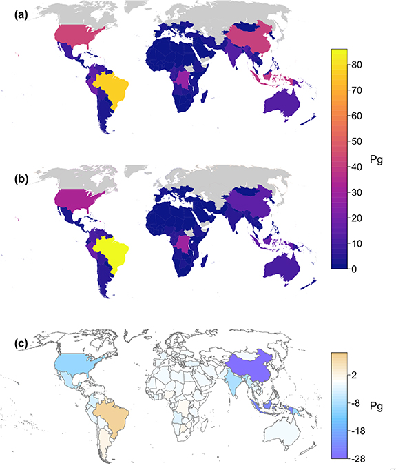
Figure 4. GEDI country-wide estimates of AGB as compared with in-country reports. (a) GEDI estimates. (b) FAO estimates. (c) Difference (FAO—GEDI). GEDI estimates AGB across all land, not just forested land, while FAO estimates are focused on forests. The national forest inventories used as the basis of FAO's estimates vary widely in terms of framework, quantity, and quality.
Download figure:
Standard image High-resolution image
Figure 5. Aboveground biomass (AGB) from GEDI and FAO by country. Solid line is 1:1; slope and R2 are found from linear regression between the two variables. RMSD (root mean square difference) is found using the difference between GEDI and FAO estimates. Data for each country is given in table S2.
Download figure:
Standard image High-resolution imageGEDI does not observe the entire global land surface, so it is not possible to estimate total AGB for the Earth. Additionally, due to data availability issues, FAO does not provide an estimate for every country where there is a GEDI estimate. For those 169 countries with both a GEDI and FAO estimate, the GEDI estimated total biomass was 480.2 Pg. FAO estimates for these same countries totalled 373.1 Pg, a total difference of 107.1 Pg. Thus, GEDI estimates about 29% more AGB for the tropical and temperate land surface compared to FAO estimates. This difference is related, in part, to the fact that GEDI measures the biomass of both forest and non-forest areas, whereas FAO estimates are only for those areas denoted as forest (>10% canopy cover of minimum 5 m height over 0.5 ha area). Incomplete filtering of anomalous waveform data, topographic artefacts, and model misspecification can also result in estimates of AGB that are too large from GEDI. These issues are addressed in GEDI data processing and are further considered in section 4.
Biomass density showed more variability than total biomass in comparisons with FAO (R2 = 0.57, RMSD = 47.7 Mg ha−1) but the relationship was influenced by a few outliers from smaller countries (figure S5). GEDI estimates were mostly higher than FAO, with 126 of the 169 countries assessed having higher AGBD from GEDI. This is again related to the factors listed above as well as the differences in how the densities are calculated. GEDI estimates are the average density over all lands, whereas FAO densities are the total biomass of lands supporting biomass, as reported by FAO, divided by the total area of the country (not just forested lands), which necessarily must lead to lower estimates of AGBD from FAO. SEs of mean AGBD were small with a mean of 3.4 Mg ha−1 (figure 6). Errors exceeding 5 Mg ha−1 occurred almost exclusively over small island nations having incomplete sampling and low biomass stocks. Two notable exceptions were Indonesia and Papua New Guinea which had AGBD errors of 7.3 Mg ha−1 and 19.3 Mg ha−1, respectively (figure 7).
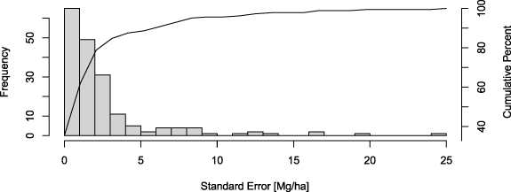
Figure 6. Country-level AGBD standard errors. Line gives the cumulative frequency.
Download figure:
Standard image High-resolution image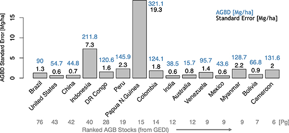
Figure 7. Standard errors for countries with the 15 largest biomass stocks (AGB) as estimated from GEDI. Above each bar is given the GEDI AGBD (blue) and its standard error (black). Stocks for each country are given below the country name.
Download figure:
Standard image High-resolution image3.3. Comparison with U.S. National Forest Inventory data
We applied hybrid inference with GEDI data to 64 000 ha hexagons covering the United States and compared our estimates to those derived from the USFS FIA plots (figure 8). There are some systematic differences apparent between the two: GEDI estimates of AGBD were low relative to FIA data in the conifer dominated PFT of the Pacific Northwest and northern East Coast regions while the mixed broadleaf forests of the Eastern U.S mountainous areas showed consistently higher AGBD in comparison to FIA. For the U.S. hexagons, GEDI data compare well to FIA estimates, with r2 = 0.81, RMSD = 28.3 Mg ha−1, and the slope of the relationship equal to 0.99 (figure 9(a)). GEDI estimated an average AGBD of 52.6 Mg ha−1 and AGB of 3.2 Tg per hexagon. The equivalent FIA estimates were AGBD of 41.9 Mg ha−1 and AGB 2.6 Tg, bearing in mind that FIA only measures biomass on lands meeting its definition of forest but density here was calculated as a function of the entire land surface area of the hexagon. The mean AGB difference (FIA—GEDI) was −0.64 Tg; GEDI thus estimates about 24.3% more biomass stock in the U.S. relative to the FIA total. This histogram of differences is negatively skewed reflecting the larger GEDI values in Eastern U.S. (figure 9(b)) and a direct comparison of quantiles shows both that GEDI estimates tend larger than FIA for values of AGBD below around 250 Mg ha−1 and smaller for values above that. Note that in contrast to country comparisons, there is little difference in the patterns and relationships using AGB or AGBD relative to FIA because the land area of every hexagon is the same, aside from a few on the coasts or the borders with Canada and Mexico.

Figure 8. Aboveground biomass density (AGBD) estimated by GEDI for the United States. (a) Mean AGBD from GEDI within hexagons. (b) Difference (FIA—GEDI) between FIA AGBD estimated from plot data and GEDI estimates for each hexagon. There are approximately 12 000 hexagons covering the coterminous U.S. and each hexagon has an area of 64 000 ha (640 km2).
Download figure:
Standard image High-resolution imageThe SEs of the mean from GEDI for hexagons as derived from hybrid estimation, along with the SEs derived from the designed-based FIA network may be used to assess the likelihood that observed hexagon-level differences are meaningful (figure 9(c)) and to compare the precision of their mean estimates through their individual confidence intervals (figure 10). Note that the hybrid estimator is not fully model-based; its distribution comes from a cross of the model-based component and a design-based component so that SEs or confidence intervals may be compared (as in McRoberts et al [37]).

Figure 9. Comparison of GEDI and FIA AGBD means in FIA hexagons. (a) Relationship between GEDI and FIA AGBD estimates for hexagons. Colors correspond to (c) below. (b) Histogram of mean hexagon AGBD differences, with inset showing the quantile-quantile plot of GEDI vs. FIA AGBD. (c) Spatial variability of the test statistic for a difference of AGBD means (FIA—GEDI). Values roughly in the range of [−2, 2] (green colors) imply that differences between the two are less likely to be significant. Increasingly orange colors suggest that the GEDI mean is likely greater than the FIA mean; increasingly purple colors suggest that the FIA mean is likely greater than GEDI. Grey areas are where there are no FIA estimates of AGBD and therefore no standard error.
Download figure:
Standard image High-resolution image
Figure 10. The 95% confidence interval widths for GEDI and FIA means at the hexagon scale. While GEDI variance estimators include both a modeling component and a sampling component, GEDI has smaller widths because it has many more footprint-level biomass predictions, thereby reducing sampling error relative to FIA which has about 28 field plots per hexagon. Note that frequency (y-axis) is on a logarithmic scale. The few GEDI confidence intervals with widths exceeding 50 Mg ha−1 are partial hexagons located on the coastlines and international borders.
Download figure:
Standard image High-resolution image
Approximately 21% of the hexagons did not have a confidence interval from FIA because the FIA AGBD estimate was zero. While the FIA assumes zero biomass for non-forest lands, GEDI estimates biomass for cells across all lands, and so has a non-zero biomass estimate for these.
The spatial distribution of a test statistic for the difference of means showed regional, systematic differences in estimated AGBD, most notably the Pacific Northwest and the Appalachian region of the Eastern U.S. GEDI generally has smaller confidence intervals about its means relative to FIA because it has many more observations within a hexagon as compared to FIA data. GEDI uncertainties also include a modelling error term from the calibration equations which is not present in FIA estimates. These modelling errors are not large and despite some dependence on the number of samples per tile and the number of models applied, remain relatively constant across scales, from 1 km cells to the areas of hexagons to entire countries. Note, however, that GEDI estimates of uncertainty do not account for any violations of the assumptions of hybrid inference, which may lead to biases and mean precisions and confidence ranges that are overly optimistic, discussed next.
4. Discussion
GEDI was conceived to provide the data on ecosystem structure required to address important questions about the Earth's forests, including quantifying the net impact of deforestation and subsequent regrowth on atmospheric CO2 concentrations, among others. Key to these efforts is the creation of accurate maps of baseline carbon stocks of sufficient spatial resolution and with well-understand uncertainties that may be used to monitor changes through time and provide accurate initialization for prognostic studies of the impacts of land use and climate change.
Several aspects unique to GEDI set the mission and its resulting biomass maps apart from others that have been produced before. First, GEDI's biomass maps are based on GEDI data alone, and are not the product of fusion or spatial extrapolation with data from other sensors. Secondly, the models that relate waveform measurements, such as height to biomass, were created using one of the most extensive sets of field and aircraft data assembled for global biomass calibrations. Third, GEDI has provided vastly more observations of ecosystem structure than previously available; our study used over 5 billion of these estimates from nearly 9000 tracks to make its products. Past studies using GLAS at country to global scales were based on one to two orders of magnitude less data [15–17]. For example, Nelson et al [17], who, using methods similar to our own, report that they used ∼940 000 ICESat shots taken from 230 orbits (where orbits are considered as cluster samples). Our estimates for the US with GEDI use ∼450 000 000 quality shots taken from nearly 4000 tracks. However, GEDI most fundamentally represents a turning point because of its focus on formalized inference. Specifically, while biomass products from previous satellites have assessed residual error uncertainty at the pixel level, GEDI recognizes the need to assess uncertainty when individual observations (pixels, for example) are combined to estimate biomass over a larger area. Residual error in that context has little relative impact compared to the uncertainty that arises due to estimating the parameters of the models linking field observations with GEDI metrics.
The model parameters themselves are a more relevant source of uncertainty under the model-based paradigm, as they affect all predictions in a systematic way. GEDI's hybrid estimator explicitly accounts for uncertainty in the model-fitting process through the use of the model's parameter covariance matrix [25]. There are alternative methods for explicitly addressing the effects of model covariance upon population estimates for large areas; for example approaches involving bootstrapping have been proposed [24]. The key is that GEDI is the first forest observation mission to embrace inference over large areas, employing an integrated design process to account for the instrument's sampling pattern, the fitting of biomass models, and the reporting of grid cell mean biomass estimates and their uncertainties. Previous remote sensing efforts that have ignored covariance among observations over large areas have had to rely upon ad hoc, and sometimes ambiguous, methods of uncertainty assessment [3, 41].
The precision requirement of the GEDI mission that 80% of 1 km cells not exceed a SE of 20 Mg ha−1 or 20% of the mean AGBD (for low and high biomass levels, respectively) has not yet been met, due to changes in the ISS altitude that led to a 4 d repeat cycle which left gaps in coverage, as discussed earlier. But as noted above, of those cells with the requisite two overpasses, 95% meet the GEDI requirements. Substantial progress with respect to meeting the 80% mission goal is expected within the next year because: (a) the precision of GEDI's estimators is expected to increase rapidly as cells accumulate more than two overpasses [25]; and, (b) recent changes to the ISS altitude are expected to substantially improve coverage of 1 km cells with no existing observations.
GEDI's variance estimates, accompanying the estimate of the mean for every 1 km cell, are crucial to monitoring progress toward the mission's precision goal. This cannot be achieved solely by validation using independent data. Validation using field data is not feasible globally and there are almost no 1 × 1 km field plots in any ecosystem, forested or otherwise. Comparison against 1 km estimates derived from airborne lidar is possible, however this process involves airborne estimates subject to some of the same model-related uncertainties affecting GEDI and would cover only a small fraction of the nearly 105 million grid cells over land in the study area. Direct comparisons with existing biomass maps are also difficult because they often have differing resolutions and, as noted above, unclear statistical procedures to estimate uncertainty from pixels to some larger area—for example, comparing a 30 m biomass product to GEDI via aggregation of the 30 m pixels to 1 km—although progress continues to be made in this area [37].
Nevertheless, comparison against independent estimates of mean AGBD provide an opportunity to highlight potential problems with GEDI's current estimation process. Some degree of spread is to be expected in the hexagon- and country-level comparisons; field estimates have their own uncertainties, and important differences in definitions and allometric models can introduce large discrepancies among estimates that would otherwise be in agreement [35]. Systematic differences between GEDI and reported estimates, though, suggest several issues worth exploring during GEDI's continued operations.
First, comparison with FAO data showed GEDI estimated more AGB for most countries. The UN FAO defines trees outside of forests and other wooded lands as those growing on lands with a combined cover of shrubs and trees of less than 10%, or tree cover less than 5%, or any trees growing in patches smaller than 0.5 ha or in urban or agricultural land. Such trees and patches are widespread in some areas [42–44] and represent biomass that is measured by GEDI but not by forest inventories. Application of standardized definitions of forest resulting in explicit and agreed upon forest/non-forest maps would enable refined comparisons. GEDI's footprint estimates of biomass could then be averaged only for forested areas for comparison to FAO estimates within countries.
Secondly, the footprint biomass calibration models linking field biomass to the GEDI waveforms are assumed under model-based estimation to be both properly specified and fitted with data representative of the areas to which the models will be applied [32]. Estimated SEs may reflect a lack of fit with respect to available training data (for example somewhat lower R2 ) but will not reflect biases in the selection of that data, and therefore potential biases in the calibration equations as applied. Comparisons with validation data can help reveal possible violations of the assumptions underlying model-based inference that are not revealed in the calibration model building process. For example, GEDI currently estimates far more AGB (a combined 51 Pg) in China and Indonesia than the countries themselves report [40]. While these positive differences may be associated with the issue of non-forest biomass discussed above, we note that GEDI's AGBD calibration dataset is particularly sparse in Asia and therefore represents a potential source of bias. This lack of data in Asia may also help explain the relatively high SEs for mean AGBD in Indonesia and Papua New Guinea; however, note that there is also a tendency for errors to increase as the magnitude of AGBD increases.
Similarly, comparison with FIA data in the western U.S. at the hexagon level reveals discrepancies that are, according to the respective confidence intervals, unlikely to be a result of sampling error on the part of GEDI or the field inventory. Some of these conifer systems may have biomass densities that exceed 2000 Mg ha−1 at the scale of GEDI footprints, and the calibration data set and derived calibration models [23] may not adequately represent the range of biomass present in this PFT as it occurs in these western montane regions. These examples indicate the need for additional data collection and a re-examination of the footprint biomass calibration models fitted for the region to refine GEDI's estimates of biomass for these areas. While improved model training in data sparse areas will help us better meet our assumptions, this may come at the cost of an increase in SEs as potentially overly optimistic estimates are corrected.
Third, there is an assumption that the height metrics, as derived from the return waveform by GEDI algorithms, are unbiased and have errors that match pre-launch calibration analyses, e.g. 1–2 m for canopy top height accuracy. The process of outlier detection, that is filtering of GEDI measurements to remove invalid data, while improving, is imperfect and errors in estimated biomass may remain. One example is misidentification of low-lying clouds that produce lidar waveforms that appear as tall canopy, an effect we noted in comparisons with FIA data in the ridge and valley complex of the Appalachians in the eastern United States. Steep topography also may lead to incorrect data interpretation. Over mostly bare-earth terrain with high slopes (generally exceeding about 15°–20°), waveforms have vertical extents that may appear similar to canopies in GEDI algorithms yet provide spurious relative height metrics that are unrelated to real canopy height. This can lead to biomass estimates that are too large, say for very sparse woodlands, or estimates for areas that cannot support vegetation, such as deserts. For forested terrain, steep slopes may increase or decrease perceived canopy height based on canopy cover and tree distributions in the footprint [45]. As GEDI outlier detection methods and waveform processing improve, such artifacts will decrease. For example, we have applied machine learning methods as an alternative to conventional waveform processing. Such methods have the potential to both increase accuracy but also provide improved error and outlier detection [46].
Comparisons such as these presented above are useful for highlighting potential modifications to biomass estimates as the mission progresses, and they also demonstrate the value of reliance upon an inferential framework where assumptions are clear and there are straightforward mechanisms through which violation of those assumptions may bias the estimates. In other words, because the framework allows for a direct estimate of the precision of its estimates, these may be used to flag deviations from validation data that are probabilistically unlikely and thus provide the means for detecting biases. As the mission works through these potential issues it may be that some new estimates of biomass are produced that are outside existing confidence intervals, reflecting a correction of bias in the process, as mentioned above. This is not a cause for concern; rather, it reflects the power of the GEDI approach.
Note that although many of the reported SEs at the country level are small, for example 1.1% for the United States, these are in line with those reported by other studies [17, 18] that used methods related to our own. However, our approach, as with these other studies and almost all national forest inventories, does not consider model uncertainty from the allometric tree-level biomass models. Such uncertainty may be substantial, especially in tropical areas [47] where the data underpinning the models tend to be limited. Thus, a formally reported SE, whether from a plot-based national inventory or one based on remote sensing, may be too optimistic considering these potentially larger allometric errors. Work is ongoing towards improving these allometric models, most recently using terrestrial lidar scanning [48].
5. Future directions and conclusions
It may seem that building a remote sensing mission upon a formal mode of inference is limiting; that is, that the necessary design considerations may limit the flexibility of future applications using its data. However, the experience of GEDI thus far has illustrated just the opposite. The orbital resonance resulting from the ISS altitude in 2020 and beyond challenged the application of hybrid inference across large areas, e.g. areas of differential probability of inclusion within the sample are not addressed by the estimators described by Patterson et al [25]. The orbital problem accentuated variable sample intensity that developed due to both the differential presence of clouds and the latitudinal differences in overpass density. This disruption was accommodated relatively simply by applying the estimators at the broadest scales for which probabilities of selection could be presumed equal (6 km tiles) and using a weighted aggregation process while accounting for dependencies due to non-independent sampling and modeling errors. This is similar to weighted averaging of smaller-domain estimates practiced by field inventories when sample intensities vary over larger domains [49].
The parametric models and sample design used by GEDI also support a type of contingency approach applicable when a 1 km cell has not been intersected by at least two ground tracks, meaning that hybrid inference (which treats ground tracks as cluster samples) is not an option. Even by the end of the mission we expect some cells to still have incomplete coverage. Our contingency approach, Generalized Hierarchical Model-Based inference (GHMB) [50, 51], uses two levels of models: one linking ground data and footprint scale lidar metrics (i.e. the footprint biomass calibration models) and one linking those footprint biomass predictions to wall-to-wall ancillary data. The GHMB framework uses probability theory under the model-based paradigm to appropriately combine uncertainty from the two models, as wall-to-wall predictions form the basis of a large-area estimate of biomass [51–53]. Thus, the theory upon which GEDI's estimation of uncertainty is built can be extended to sensor fusion. For example, GHMB has been used with GEDI and wall-to-wall imagery from TanDEM-X [54], which provides interferometric synthetic aperture radar (SAR) from two orbiting satellites, to produce both height and biomass estimates for areas where no GEDI data exist, and at finer spatial resolutions than 1 km [51]. One strong feature of GHMB is that models relating GEDI data to the wall-to-wall data may be locally calibrated. The GEDI team intends to use GHMB to provide gap-free biomass maps in subsequent data product releases. This framework further provides a pathway for fusion with the next generation of SAR missions with science goals related to biomass and disturbance dynamics, including the NASA ISRO Synthetic Aperture Radar mission (NISAR) [55] to be launched in 2024 and the ESA BIOMASS mission [56], scheduled for launch in 2023.
In conclusion, GEDI has demonstrated the value of an instrument dedicated to and optimized for the retrieval of ecosystem structure in general, and for biomass estimation in particular. The sheer volume of GEDI estimates of biomass is unprecedented, vastly outstripping the existing spaceborne lidar archive. GEDI's estimates continue to evolve as the instrument collects more data beyond its prime mission, and as footprint-level biomass models and their underlying assumptions are refined in light of ongoing validation activities. The results reported here represent a watershed product of the first space mission longitudinally coordinated, from engineering to estimation, to generate biomass products in a transparent way with errors that are well-characterized using established probability theory. The GEDI investigation highlights the intrinsic value of an approach that explicitly addresses uncertainty as integral part of mission design. As GEDI and future missions invest in formal modes of inference, they bring statistical rigor long employed by field surveys to a new generation of powerful, globally consistent monitoring tools.
Acknowledgments
We gratefully acknowledge the numerous collaborators who generously contributed field estimates of AGBD, stem maps, and airborne lidar data. These people include Katharine Abernethy, Hans-Erik Andersen, Paul Aplin, Timothy R Baker, Nicolas Barbier, Jean Francois Bastin, Pascal Boeckx, Jan Bogaert, Luigi Boschetti, Peter Brehm Boucher, Doreen S Boyd, Patrick Burns, David F R P Burslem, Sofia Calvo-Rodriguez, Jérôme Chave, Robin L Chazdon, David B Clark, Deborah A Clark, Warren B Cohen, David A Coomes, Piermaria Corona, K C Cushman, Mark E J Cutler, James William Dalling, Michele Dalponte, Sergio de-Miguel, Songqiu Deng, Peter Woods Ellis, Barend Erasmus, Michael Falkowski, Patrick A Fekety, Alfredo Fernández-Landa, Antonio Ferraz, Rico Fischer, Adrian G Fisher, Antonio García-Abril, Terje Gobakken, Jonathan A Greenberg, Jorg M Hacker, Marco Heurich, Ross A Hill, Sören Holm, Chris Hopkinson, Chengquan Huang, Huabing Huang, Stephen P Hubbell, Andrew T Hudak, Benedikt Imbach, Patrick Jantz, Kathryn Jeffery, Masato Katoh, Elizabeth Kearsley, Natascha Kljun, Nikolai Knapp, Kamil Král, Martin Krůček, Nicolas Labrière, Seung-kuk Lee, Simon L Lewis, Marcos Longo, Richard M Lucas, Russell Main, Jose A Manzanera, Suzanne Marselis, Rodolfo Vásquez Martínez, Renaud Mathieu, Victoria Meyer, Paul Montesano, Felix Morsdorf, Erik Næsset, Laven Naidoo, Reuben Nilus, Michael J O'Brien, David A Orwig, Geoffrey Parker, Christopher Philipson, Oliver L Phillips, Jan Pisek, John R Poulsen, Wenlu Qi, Christoph Rüdiger, Sassan Saatchi, Arturo Sanchez-Azofeifa, Nuria Sanchez-Lopez, Crystal B Schaff, Marc Simard, Andrew Kerr Skidmore, Göran Ståhl, Krzysztof Stereńczak, Chiara Torresan, Rubén Valbuena, Hans Verbeeck, Tomas Vrska, Konrad Wessels, Joanne C White, and Carlo Zgraggen.
We also thank Suzanne Marselis, David Minor, and Carlos E Silva for contributing to the development and management of the GEDI Forest Structure and Biomass Database and Timothy Gregoire, Ron McRoberts, Eric Næsset and Ross Nelson for discussions on the GEDI statistical estimation framework.
Data availability statement
The GEDI footprint biomass data used to create the GEDI L4B 1 km gridded data product are available at the Land Processes Distributed Archive and Analysis Center (LPDAAC) as follows: GEDI L4A Footprint Level Aboveground Biomass Density, Version 2. (2021) doi: 10.3334/ORNLDAAC/1986. The GEDI country-level data are included in the Supplements. The GEDI results for mean and standard error of U.S. hexagons can be obtained by request from Ralph Dubayah.
The data that support the findings of this study are openly available at the following URL/DOI: https://doi.org/10.3334/ORNLDAAC/2017.
Funding
NASA Contract #NNL15AA03C for the development and execution of the GEDI mission.
Author contributions
This paper was conceived and written by Ralph Dubayah, Sean Healey, and John Armston with contributions from Jamis Bruening. The hybrid estimates of biomass were produced by John Armston with contributions from Svetlana Sareela, Göran Ståhl, Paul Patterson, and Zhiqiang Yang. Svetlana Saarela and Göran Ståhl developed the estimators for large area estimation that are presented in the Supplementary Methods, with contributions from Sean Healey, John Armston, Zhiqiang Yang and Ralph Dubayah. The analysis of the FIA and GEDI hexagon comparisons were led by Jamis Bruening, Ralph Dubayah, Sean Healey, and John Armston. All other authors contributed to the editing of the manuscript and played a fundamental role in developing critical GEDI data, processing, and analytical assets.
Conflict of interest
Authors declare that they have no competing interests.
Supplementary data (PDF)