

Abstract
Atmospheric carbon dioxide (CO2) concentrations have increased as a direct result of human activity and are at their highest level over the last 2 million years, with profound impacts on the Earth system. However, the magnitude and future dynamics of land and ocean carbon sinks are not well understood; therefore, the amount of anthropogenic fossil fuel emissions that remain in the atmosphere (the airborne fraction) is poorly constrained. This work aims to quantify the sources and controls of atmospheric CO2, the fate of anthropogenic CO2 over time, and the likelihood of a trend in the airborne fraction. We use Hector v3.0, a coupled simple climate and carbon cycle model with the novel ability to explicitly track carbon as it flows through the Earth system. We use key model parameters in a Monte Carlo analysis of 15 000 model runs from 1750 to 2300. Results are filtered for physical realism against historical observations and CMIP6 projection data, and we calculate the relative importance of parameters controlling how much anthropogenic carbon ends up in the atmosphere. Modeled airborne fraction was roughly 52%, consistent with observational studies. The overwhelming majority of model runs exhibited a negative trend in the airborne fraction from 1960–2020, implying that current-day land and ocean sinks are proportionally taking up more carbon than the atmosphere. However, the percentage of atmospheric CO2 derived from anthropogenic origins can be much higher because of Earth system feedbacks. We find it peaks at over 90% between 2010–2050. Moreover, when looking at the destination of anthropogenic fossil fuel emissions, only a quarter ends up in the atmosphere while more than half of emissions are taken up by the land sink on centennial timescales. This study evaluates the likelihood of airborne fraction trends and provides insights into the dynamics of anthropogenic CO2 in the Earth system.
Export citation and abstract BibTeX RIS
1. Introduction
We are witnessing unprecedented changes to the climate. In 2019, atmospheric carbon dioxide (CO2) levels were the highest they have been in the last two million years (Masson-Delmotte et al 2021). Global surface temperature has increased faster between 1970–2020 than in any other 50 year period in the last two thousand years (Masson-Delmotte et al 2021). Both anthropogenic emissions and atmospheric CO2 concentrations are rising, with the latter increasing to approximately 412 ppm in 2020 (Friedlingstein et al 2020). These changes are affecting all major components of the climate system (Masson-Delmotte et al 2021).
As the Earth warms, the proportion of CO2 taken up by natural ocean and land sinks is expected to decrease, resulting in more anthropogenic emissions in the atmosphere (Masson-Delmotte et al 2021). The airborne fraction is an estimate of the amount of anthropogenic CO2 emissions that accumulate in the atmosphere, as opposed to emissions that are transferred to the land and oceans. The airborne fraction has long been a focus of study as it is a useful summary statistic reflecting human influence on CO2 concentrations. Several studies suggest that around 45% of anthropogenic CO2 remains in the atmosphere and that this figure has remained relatively constant over the last several decades, noting that there is significant uncertainty in establishing a trend (Poulter et al 2011, Ballantyne et al 2012, Jones et al 2013, van Marle et al 2022). However, we may soon approach a point where natural sinks are not able to take up as much CO2 as is emitted into the Earth system. This would result in additional CO2 in the atmosphere and therefore, heightened climate impacts (Jones et al 2013, van Marle et al 2022).
Likely future changes in the airborne fraction, and behavior of the ocean and land sinks that drive it, can be analyzed with carbon and climate models. Such models are a primary aid for studying the Earth system and vary in computational power and resolution. More complex coupled Earth system models (ESMs) are a powerful tool in Earth system science, although they are computationally expensive (Nicholls et al 2021). In contrast, reduced complexity or simple climate models are computationally efficient with a lower spatial and temporal resolution than ESMs, meaning they can be run quickly and used for large ensembles of multiple scenarios (Nicholls et al 2020). Many simple climate models, including the model used in this study, exist that operate in good agreement with results from Coupled Model Intercomparison Project phase 6 (CMIP6) ESM runs (e.g. MAGICC, Meinshausen et al 2011; RCMIP, Nicholls et al 2021; OSCAR, Quilcaille et al 2022; FAIR, Smith et al 2018; Hector, Hartin et al 2015).
This analysis uses the open-source, object-oriented, simple global carbon cycle climate model Hector (Hartin et al 2015). We use Hector v3.0's novel carbon tracking feature to understand the sources of current and future atmospheric CO2, the destination of anthropogenic CO2 on centennial timescales, what factors control how much CO2 ends up in the atmosphere, and the uncertainties on the trend and robustness of airborne fraction as a metric for studying carbon cycle feedbacks.
2. Methods
2.1. Model description
Hector is an open-source, object-oriented, simple global carbon cycle climate model, one of many reduced complexity climate models (Nicholls et al 2021). As a simple climate model, Hector runs very quickly while still representing the most critical global Earth system processes. Hector can accurately reproduce historical trends and model future projections of atmospheric CO2, radiative forcing, and global temperature change under the representative concentration pathways (RCPs) and shared socioeconomic pathways (SSPs) in addition to other user-defined scenarios. Hector v2.0 improved the model's vertical ocean structure, heat uptake, and surface temperature response to radiative forcing and incorporated a semi-empirical model based on global temperature to calculate global sea level change (Vega-Westhoff et al 2019). For a more comprehensive model overview, please reference the supplementary material S1.
Hector v3.0 incorporates several scientific advances and introduces new features to the model, including a permafrost implementation, user-defined land-ocean warming contrast, and a carbon tracking feature. Hector v3.0's default parameter set is calibrated against the observational record: the model is run by an optimizer that varies key input parameters and attempts to minimize the error between the model and historical CO2 and temperature observations; this is described in Dorheim et al (2023). Calibration procedures vary widely for simple climate models, but such an approach is common (Meinshausen et al 2011, Tsutsui 2020).
2.2. Carbon tracking
This analysis leverages the carbon tracking capability introduced in Hector v3.0, which allows the user to trace the flows of carbon as the model runs without affecting model behavior. Tracking only considers atmospheric carbon in the form of CO2, not other greenhouse gases. At a user-defined 'start-tracking' date, the model marks all carbon in each of its pools as self-originating, meaning at that point, for example, the soil pool is deemed to be composed of 100% soil-origin carbon. As the model runs and carbon is exchanged between the various pools, the origin of all carbon is retained. At the end of a run, one can extract detailed information about the composition of each pool at each time point, including what fraction of the pool is sourced from which other pools. Hector traces carbon through eight atmospheric, terrestrial, and oceanic pools; a ninth pool, 'earth_c', represents CO2 from fossil sources injected into the carbon cycle as anthropogenic emissions. In this analysis, 'anthropogenic emissions' refers only to fossil fuel and industrial emissions and does not include land use change (LUC) emissions.
2.3. Parametric uncertainty
We create random parameter draws from Hector default parameters and a priori uncertainties from literature and perform a 15 000 run Monte Carlo simulation, a procedure used in other simple climate model experiments (Smith et al 2018, Quilcaille et al 2022). We explore model results in the Tier 1 joint SSP-RCP scenarios outlined in O'Neill et al (2016); we broadly refer to these as 'scenarios' or 'SSPs' hereafter. We consider a run to be one Hector model run from 1750–2300 with a unique combination of parameter values. All runs are emission-driven, i.e. in which the model must compute the atmospheric concentration of greenhouse gas from anthropogenic emissions accounting for Earth system feedbacks, rather than operate from prescribed concentrations (Meinshausen et al 2020); it thus provides a more stringent test for the model. Hector runs with an annual timestep and for the setup used here, there is a single global biome with no further spatial resolution. Note that carbon tracking was turned on in 1750 for each run. The parameters and their assumed distributions are given in table 1.
Table 1. Hector model parameters included in the Monte Carlo uncertainty analysis, where the distribution represents the mean value ± the standard deviation. These are standard parameters for simple global climate models (Meinshausen et al 2011). For each model run (per-scenario N = 3 750), a random value for each parameter was drawn from its corresponding distribution.
| Parameter | Description | Units | Distribution | Source of uncertainty |
|---|---|---|---|---|
| AERO_SCALE | Aerosol forcing scaling factor | Unitless | 1.0 ± 0.23 (Normal) | Smith et al (2020) |
| β | CO2 fertilization factor, the degree to which plant productivity increases under elevated CO2 as photosynthesis becomes more efficient and less water-limited | Unitless | 0.55 ± 0.10 (Normal) | Jones et al (2013) |
| ECS | Equilibrium climate sensitivity | °C | 3.0 ± 0.65 (Lognormal) | Sherwood et al (2020) |
| LUC_SCALE | Land use change emissions scaling factor | Unitless | 1.3 ± 0.2 (Lognormal) | Friedlingstein et al (2020) |
| κeff | Ocean vertical diffusivity | cm2 s−1 | 1.18 ± 0.23 (Normal) | Vega-Westhoff et al (2019) |
| NPP0 | Pre-industrial net primary productivity | Pg C yr−1 | 56.2 ± 14.3 (Normal) | Ito (2011) |
| Q10 | Temperature sensitivity of heterotrophic respiration | Unitless | 2.16 ± 1.0 (Lognormal) | Davidson and Janssens (2006) |
| TT | Thermohaline overturning | m3 s−1 | 7.2 × 10⁷ ± 7.2 × 10⁶ (Normal) | Hartin et al (2015) |
| TU | High-latitude overturning | m3 s−1 | 4.9 × 10⁷ ± 4.9 × 10⁶ (Normal) | Hartin et al (2015) |
| TWI | Warm-intermediate exchange | m3 s−1 | 1.25 × 10⁷ ± 1.25 × 10⁶ (Normal) | Hartin et al (2015) |
| TID | Intermediate-deep exchange | m3 s−1 | 2 × 10⁸ ± 2 × 10⁷ (Normal) | Hartin et al (2015) |
We introduce an LUC emissions scaling parameter to account for large uncertainties in LUC emissions. Friedlingstein et al (2020) found that cumulative CO2 emissions from LUC for 1850–2020 totaled 200 ± 65 GtC, although when looking at a spread of models, values ranged from 140 GtC to 270 GtC (Friedlingstein et al 2020). In Hector, cumulative LUC emissions over the same period total ∼168 GtC for our central setup. To scale this value to align with the range above, we chose a lognormal distribution (to exclude any negative or near-zero values) of 1.3 ± 0.2. LUC emissions in Hector were then multiplied by the randomly-drawn scaling parameter value for each Hector run.
In the real world, some of the processes described by the parameters in table 1 are likely to covary (Forest et al 2002, Sansó and Forest 2009), reflecting coupling or feedbacks that exist but are not well understood. Rather than attempt to define a priori the shape and strength of these covariances (e.g. Leach et al 2021), we elected to vary each parameter independently of the others, i.e. without any predefined correlations, and then used a stringent run-filtering step to ensure that the model runs used in the analysis were physically realistic, following e.g. Goodwin (2016). That is, the effect of any parameter correlations would emerge as the posterior ensemble was generated.
2.4. Filtering model runs for physical realism
Particular combinations of parameters can produce physically unrealistic runs, i.e. outputs that diverge greatly from either the observational record or the broad envelope of CMIP6 future runs. This problem is common in random ensembles of simple model runs (Nicholls et al 2021), and procedures for extracting the posterior ensemble from the prior ensemble vary considerably (Goodwin 2016, Leach et al 2021). Following studies such as Dvorak et al (2022), we subjected model runs to a four-part filter by comparing them against CO2 concentrations, temperature, land-atmosphere carbon exchange, and ocean-atmosphere carbon exchange:
- We use historical data to constrain CO2 concentration. Minimum and maximum 'acceptable' bounds were set for the historical period (1959–2014) by adding and subtracting the standard deviation of CMIP6 runs to the NOAA observational historical mean (Tans and Keeling 2023). We do not use future CO2 as a filter primarily due to limited emissions-driven projection data.
- For the global temperature anomaly, we use the mean, minimum, and maximum values of the CMIP6 runs from 1850–2014 (historical) and 2015–2100 (future). We use the CMIP6 mean in lieu of global temperature observations to constrain historical temperature because the mean reproduces historical temperature very well (Fan et al 2020, Papalexiou et al 2020, Arias et al 2021).
- Two additional filters were the land-atmosphere and land-ocean carbon exchange values from the Global Carbon Project (Friedlingstein et al 2022). These are model results, not observations; use LUC assumptions that differ significantly from those of Hector, which are consistent with the RCMIP project (Nicholls et al 2021); and, importantly, are driven by observed climate. The ensembles thus have a very small range that, when coupled with the year-to-year variabilities of these carbon sinks, meant that essentially no Hector run could 'pass' these particular filters. For this reason, we multiplied the GCP-reported standard deviations by 3.0, an arbitrary value but one that produced a model spread comparable to the others described above while still providing a stringent filter for physical realism.
In all of the filtering steps, if more than 50% of values from a particular Hector run fell outside the minimum and maximum bounds, the run was considered unrealistic and removed from the dataset. Each run needed to pass all four filters to be included in our results. Such an 'accept/reject' step is commonly used, although more sophisticated approaches involving weighting of model runs also exist (e.g. Goodwin and Cael 2021). The combination of these tests results in 70% of total runs being excluded (10 538/15 000). Table 2 details the number and percent of runs that failed by each filter, and figure 1 illustrates our approach.
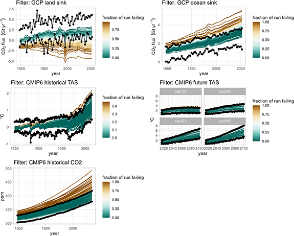
Figure 1. A summary of the model filtering process. Model output runs were compared to target ranges across the five parameters and either 'passed' or 'failed' depending on the percentage of the run that fell within the bounds over time. The black dots represent the CMIP6 projections or GCP observations. Blue lines represent passing runs while brown lines represent failing runs; the legend indicates what fraction of the run falls out of bounds.
Download figure:
Standard image High-resolution imageTable 2. A summary of the number and percent of runs that fail by each filter.
| Filter | Number of runs failing | Percent of runs failing |
|---|---|---|
| Historical CO2 | 5987 | 40.1% |
| Historical temperature | 178 | 1.2% |
| Future temperature | 504 | 3.4% |
| Land sink | 10 326 | 69.2% |
| Ocean sink | 4555 | 30.5% |
2.5. CMIP6 data
The CMIP6 data used in this analysis included 20 models for the temperature data and nine models for the CO2 concentration data from the ScenarioMIP project 4 . A different number of models were used between the two metrics due to how many models were found with consistent output. All data used was derived from emissions-driven runs. The data was downloaded and processed using Pangeo, a software ecosystem designed to enable Big Data geoscience research (Abernathey et al 2017). For the full processing workflow, please reference this repository: https://github.com/JGCRI/hector_cmip6data.
2.6. Statistical analysis
We use the R package relaimpo (v2.2.6; Groemping 2006) to calculate variance decomposition and analyze the levels of control of the individual parameters over the destination of anthropogenic emissions. We fit the 'destination fraction' of emissions to a linear model and apply a function that extracts the relative importance. This metric refers to the R2 contribution of each regressor, averaged over the different potential combinations of regressor order to eliminate dependence on regressor order. The contributions are normalized to sum to 1, meaning the influence of different parameters can be directly compared (Groemping 2006).
2.7. Airborne fraction calculation
To determine the airborne fraction, we follow convention and compute the change in the amount of atmospheric CO2 divided by the sum of emissions over the same period (Knorr 2009, Ballantyne et al 2012, van Marle et al 2022). This work only uses the sum of anthropogenic emissions and does not account for LUC emissions, as the former represents truly new carbon being injected into the global carbon cycle (Ballantyne et al 2012). Separately, because airborne fraction is commonly used as an estimate for the fraction of anthropogenic emissions remaining in the atmosphere (Knorr 2009, Poulter et al 2011, Ballantyne et al 2012, Keenan et al 2016, van Marle et al 2022), we use carbon tracking to compute this approximation. Because the airborne fraction equation does not account for anthropogenic CO2 that cycles through terrestrial or oceanic reservoirs before returning to the atmosphere, it is not a perfect estimate of this metric. We use tracking data to trace carbon emitted from the human emissions pool and calculate the fraction that resides in the land, ocean, and atmosphere pool. In contrast to airborne fraction, this provides an unambiguous tracing of anthropogenic carbon movement in the Earth system. Over short timescales, this method approximates airborne fraction, and over longer timescales, it precisely resolves the routing and destinations of anthropogenic carbon.
This analysis was performed in R 4.1.0 (R Core Team 2021) using Hector v3.0 (Dorheim et al (2023), DOI 10.5281/zenodo.7617326). The repository for Hector can be found here: https://github.com/JGCRI/hector.
3. Results
3.1. Sources of atmospheric CO2
Hector's carbon tracking feature allows the user to trace carbon as it flows through the model's carbon cycle. Figure 2 highlights this capability and shows the composition of the atmosphere by source pool over time. For clarity, we only show SSP2-45 as a 'middle of the road' scenario, although patterns are broadly consistent across scenarios. The atmosphere's 'anthropogenic emissions' pool is the only one that increases in the long term, meaning future atmospheric carbon is increasingly anthropogenic in origin. We find this trend consistent across scenarios (figure 3). In a low emissions scenario, anthropogenic emissions may compose 38% of the atmosphere, but in a high emissions case, the atmosphere pool could contain over 93% anthropogenic carbon by 2300, as CO2 from emissions is repeatedly cycled through the Earth system and back to the atmosphere.
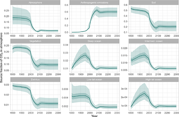
Figure 2. Fraction of CO2 in the atmosphere by source pool in SSP2-45. The lines show the median; darker shaded areas show ±1 standard deviation (s.d.) of the median and lighter areas show the minimum and maximum of the ensemble. For each run, the values of the different source pools sum to one at any point in time. We show data beginning in 1800 instead of 1750 due to an artifact that appears as the model calibrates immediately after tracking is turned on.
Download figure:
Standard image High-resolution image
Figure 3. Fraction of atmospheric CO2 from anthropogenic emissions over time across scenarios. The line shows the median and the shaded areas show ±1 s.d. of the median.
Download figure:
Standard image High-resolution image3.2. Destination of anthropogenic emissions
In addition to using carbon tracking to analyze the composition of one individual pool, we can track the destination of carbon from a particular pool. By tracking the destination of human emissions (figure 4), we find that the land sink consistently takes up most of this carbon, with the atmosphere and ocean taking up roughly comparable amounts (62%, 21%, and 17% respectively for SSP2-45 in 2300; table 4). In the long term, the ocean pool begins to increase as a sink, with a delayed response as carbon cycles more slowly with the ocean.
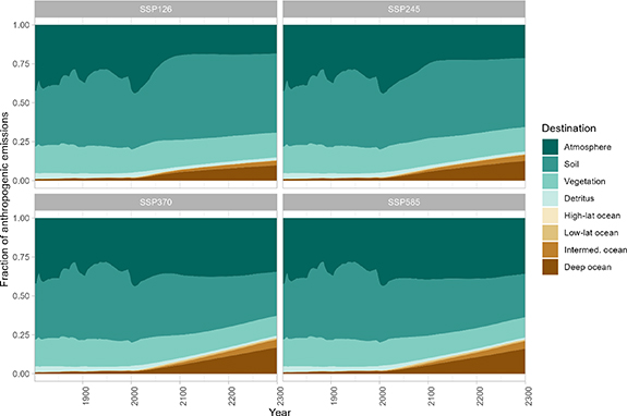
Figure 4. Destination pools of anthropogenic emissions averaged over all runs for each of the four scenarios.
Download figure:
Standard image High-resolution imageWe then analyze which of Hector's parameters has the greatest influence in controlling how much anthropogenic carbon ends up in the atmosphere over time (figure 5). Pre-industrial net primary productivity (NPP0) dominates until about 2100. Q10, the sensitivity of soil respiration to temperature, exhibits a larger relative importance across scenarios after about 2100. The CO2 fertilization factor (β), equilibrium climate sensitivity (ECS), and LUC emissions also have a nontrivial influence. The remaining parameters do not have an appreciable influence on these timescales.

Figure 5. Relative importance of model parameters (cf table 1) over time in controlling what fraction of anthropogenic emissions are in the atmosphere, by scenario. The importance metric is scaled 0–1 (Groemping 2006); for example, pre-industrial NPP is responsible for about 75% of the variability in 2000.
Download figure:
Standard image High-resolution image3.3. Airborne fraction and anthropogenic CO2
Airborne fraction is defined as the change in atmospheric carbon divided by the sum of emissions in the same period (Ballantyne et al 2012). However, airborne fraction is commonly referred to as the fraction of emissions that remain in the atmosphere, as opposed to the land/ocean sinks. We use carbon tracking to compute this. Figure 6 displays the atmospheric anthropogenic CO2 across scenarios, calculated conventionally and by using the carbon tracking outputs.
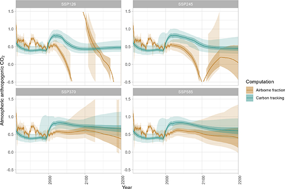
Figure 6. Atmospheric anthropogenic CO2 over time, by scenario. The blue line and band show the amount of anthropogenic emissions remaining in the atmosphere from the model's carbon-tracking mechanism, whereas the brown line and band show the actual airborne fraction computed following Ballantyne et al (2012).
Download figure:
Standard image High-resolution imageWe find that the definition of airborne fraction does not align with the colloquial expression ('the fraction of emissions remaining in the atmosphere'), as a fraction cannot be larger than one and the results diverge if there are no emissions in a timestep. The airborne fraction calculation assumes monotonically increasing emissions, which is not a given. We see this variation most dramatically in SSP1-26 and SSP2-45.
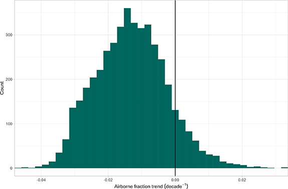
Following van Marle et al (2022), we compute the airborne fraction decadal trend between 1960 and 2020 across all runs. We determine the mean airborne fraction trend to be −0.01 ± 0.01 decade−1, and Hector overall overwhelmingly returns a negative airborne fraction trend (figure 7); 89% of the runs return a negative value.
Figure 7. The distribution of airborne fraction decadal trend values (1960–2020) across all runs and scenarios. We find a mean trend of −0.01 ± 0.01.
Download figure:
Standard image High-resolution image
4. Discussion
4.1. Sources of atmospheric CO2
We find that anthropogenic CO2 will comprise approximately 39% to 88% of the atmosphere in 2100, depending on the SSP. This variation is due to the differences within the scenarios themselves, as there are increasing emissions from SSP1 to SSP5, which result in a higher anthropogenic fraction. Table 3 summarizes the mean percentages of atmospheric CO2 by scenario. Additionally, across scenarios, the only pool that increases as a source is the anthropogenic emissions pool. By 2100, anthropogenic emissions are the majority source of atmospheric CO2 for all scenarios except SSP1-26. These model results are generally consistent with isotopic analyses of the atmosphere (Ghosh and Brand 2003, Graven 2015).
Table 3. Mean percent of atmospheric CO2 sourced from anthropogenic emissions by scenario. Note that while 2015 is a historical year, the slight variation in output is due to the parametric variability across scenarios stemming from the initial random draws.
| Year | SSP1-26 | SSP2-45 | SSP3-70 | SSP5-85 |
|---|---|---|---|---|
| 2015 | 40.4% | 40.5% | 40.4% | 40.2% |
| 2050 | 45.9% | 59.0% | 64.4% | 68.1% |
| 2100 | 38.7% | 60.0% | 80.6% | 87.6% |
| 2300 | 38.3% | 59.7% | 88.1% | 92.7% |
4.2. Destination of anthropogenic emissions
The land sink takes up most of the anthropogenic carbon across scenarios while the ocean increases as a sink in the long term. For an overview of CO2 destination by sink and scenario in 2300, see table 4. We find that 38%–93% of the atmosphere is sourced from anthropogenic emissions in 2300. However, only 19%–36% of anthropogenic emissions have the atmosphere as a destination in 2300. In a model intercomparison study, Archer et al (2009) found that 20%–35% of contemporary anthropogenic CO2 ultimately remains in the atmosphere after equilibrium with the ocean. Our 2300 values align with the lower end of that range in higher emissions scenarios, although with the caveat that Hector has not yet reached equilibrium in 2300 and that the ocean may proportionally take up more CO2 with time. We find that the land sink takes up 42%–68% of anthropogenic CO2 in 2300. With Hector's carbon tracking feature, we can distinguish between sources that are not isotopically differentiable, such as the soil and vegetation pools. This allows for a more detailed analysis of terrestrial carbon cycle dynamics and highlights the importance of future work in this area.
Table 4. Destination of anthropogenic CO2 in 2300 by sink and scenarios. Percentages across scenarios may not sum to 100% exactly due to rounding.
| Scenario | Atmosphere | Land | Ocean |
|---|---|---|---|
| SSP1-26 | 18.5% | 68.3% | 13.2% |
| SSP2-45 | 21.3% | 61.6% | 17.1% |
| SSP3-70 | 34.5% | 42.2% | 23.2% |
| SSP5-85 | 35.9% | 42.0% | 22.1% |
The pre-industrial level of terrestrial NPP0 was the dominant control on how much CO2 ended up in the atmosphere until about 2100, with the temperature sensitivity of heterotrophic respiration (Q10) dominating in the long term. In general, CO2 fertilization (β), ECS, and LUC emissions were of limited importance. Other parameters had a much smaller influence.
The initial large influence of NPP0 can be partially attributed to its uncertain distribution (table 1; Ito 2011) with a large standard deviation at nearly 25% of the mean. This allowed for a wide range of values in the Monte Carlo simulation, thereby amplifying its influence. That is not to diminish the importance of NPP0, as it is still one of the largest carbon fluxes in the Earth system, albeit with a wide uncertainty range (Friedlingstein et al 2020).
The limited effects of β are due to the empirical form of the β formulation used in Hector that, by design, saturates as CO2 increases (Hartin et al 2015). Conversely, the effect of Q10 increases exponentially with temperature; as the planet warms, there is a large increase in the rate of heterotrophic respiration, contributing to a positive climate feedback (Davidson and Janssens 2006). Furthermore, a slowdown in the CO2 fertilization effect in recent decades has been suggested (Wang et al 2020, Winkler et al 2021), which is consistent with the β effect attenuation over time as represented in Hector for the late 21st century (figure 5).
ECS, a measure of the amount of warming after a doubling of CO2 emissions, begins to increase in relative importance past 2100 as emissions increase. LUC emissions remain relatively constant in their importance, although for high emissions scenarios where the importance of other parameters increases more dramatically, LUC emissions become proportionately less influential.
4.3. Airborne fraction
The mean airborne fraction trend from 1960–2020 is −0.01 decade−1, and the spread of results indicates that a trend for contemporary airborne fraction is highly likely to be negative. This is consistent with Keenan et al (2016), who infer a similarly declining trend for the post-2000 period. Vakilifard et al (2022) found a declining late-21st-century airborne fraction trend during the negative or zero emission phase of the scenario. Additionally, van Marle et al (2022) reported that airborne fraction has decreased slightly since 1959 with a trend of −0.014 ± 0.010 per decade from 1960–2020. However, there is still significant uncertainty around airborne fraction trends. Neither Knorr (2009) nor Friedlingstein et al (2020) found any significant trend in the contemporary airborne fraction over the same period, with the latter calculating a 1960–2020 mean airborne fraction of ∼45% with large interannual variability. We compute a mean of 52% across all runs and scenarios over the same period; the divergence could be due to Friedlingstein et al (2020) including LUC emissions in the calculation of airborne fraction whereas we do not.
Figure 6 illustrates the limitations of the definition of airborne fraction, which breaks down as emissions go to zero. In our approximation metric, we see an average value of around 0.5 with some variation across scenarios, and a spike in contemporary years (∼1950–2050). This is due to a sudden increase in the rate of emissions in a short time span, which would not allow for CO2 to be taken up by the land or ocean. With time, the CO2 can enter the rest of the carbon cycle, and the approximation returns to lower values, more consistent with the range of values usually quoted for contemporary airborne fraction (e.g. Knorr 2009).
4.4. Limitations and caveats
One factor in computing airborne fraction is whether or not to include LUC emissions in the calculation. Including LUC emissions allows for a more comprehensive representation of carbon and anthropogenic influences in the Earth system, while excluding LUC allows for a sharper focus on fossil fuel and industrial emissions. For the latter reason, we do not account for LUC emissions in the airborne fraction. However, LUC emissions have historically contributed substantially to changes in atmospheric CO2; Reick et al (2010), and Ballantyne et al (2012) found that trends in airborne fraction are highly sensitive to the inclusion of LUC emissions.
For this reason, our corresponding land-borne and ocean-borne fractions over the historical period differ from those of Friedlingstein et al. We calculate these fractions to be 15% and 33%, respectively, while Friedlingstein et al (2020) reports values of 30% and 25% when including LUC emissions. With differing computation methods, this is not a direct comparison, and we expect some divergence; it is beyond the scope of the manuscript to explore this further, although this may be an interesting area of future work.
The above leads to further questions about the definition of airborne fraction, as there is a distinction between the calculation of airborne fraction and how the term is used as 'the fraction of emissions that remains in the atmosphere.' The debate over the inclusion or omission of LUC emissions further complicates this, as computed airborne fraction values (or ocean- and land-borne fractions) may differ between studies depending on the system boundary used. Furthermore, non-trivial land-atmosphere feedbacks that are not accounted for in the airborne fraction equation further contribute to the non-alignment between the definition and colloquial use of airborne fraction. As such, there needs to be greater standardization and clarity as to how each author defines airborne fraction.
An additional limitation concerns Hector, as like all models, it has areas of strength and weakness. Hector is a simple global model running on an annual timestep, meaning that we are not able to examine potentially illuminating seasonal dynamics relevant to airborne fraction and the carbon cycle (e.g. Bastos et al 2020). Hector's ocean component solves for the solubility pump without accounting for the presence of biological carbon fluxes or the response of ocean circulation and physical ventilation to climate change. This requires higher values for our ocean parameters that relate to volume transport and ventilation than those used in the CMIP6 models, compounded by the need to compensate for the lack of carbon transferred to the ocean interior by the biological carbon pump.
Acknowledgments
This research was supported by the U.S. Department of Energy, Office of Science, as part of research in MultiSector Dynamics, Earth and Environmental System Modeling Program. The Pacific Northwest National Laboratory is operated by Battelle for the US Department of Energy (Contract No. DE-AC05-76RLO1830).
Data availability statement
The data that support the findings of this study are openly available at the following URL: https://github.com/JGCRI/trackingC, see also Pressburger and Bond-Lamberty (2023), https://doi.org/10.5281/zenodo.7818565.
Author contributions
This study was conceived and designed by L P and B B-L. L P performed coding, model runs, and data analysis, working with an early version of Hector v3.0 developed by K D and others; T K, H M, and S S provided expertise on atmospheric dynamics, carbon dioxide fertilization, and the SSP scenarios. L P led the writing of the manuscript with contributions from all authors.
Footnotes
- 4
CMIP6 temperature models include: ACCESS-CM2, AWI-CM-1-1-MR, BCC-CSM2-MR, CAMS-CSM1-0, CanESM5, CAS-ESM2-0, CESM2-WACCM, CESM2, CMCC-CM2-SR5, CMCC-ESM2, FGOALS-g3, GISS-E2-1-G, IITM-ESM, MIROC-ES2L, MIROC6, MPI-ESM1-2-HR, MPI-ESM1-2-LR, MRI-ESM2-0, TaiESM1, and UKESM1-0-LL.
CMIP6 CO2 models include: BCC-CSM2-MR, BCC-ESM1, CESM2-FV2, CESM2-WACCM-FV2, CESM2-WACCM, CESM2, CNRM-ESM2-1, GFDL-ESM4, and MRI-ESM2-0.
Supplementary data (0.3 MB PDF)