


Abstract
The global recognition of modern agricultural practices' impact on the environment has fuelled policy responses to ameliorate environmental degradation in agricultural landscapes. In the US and the EU, agri-environmental subsidies (AES) promote widespread adoption of sustainable practices by compensating farmers who voluntarily implement them on working farmland. Previous studies, however, have suggested limitations of their spatial targeting, with funds not allocated towards areas of the greatest environmental need. We analysed AES in the US and EU—specifically through the Environmental Quality Incentives Program (EQIP) and selected measures of the European Agricultural Fund for Rural Development (EAFRD)—to identify if AES are going where they are most needed to achieve environmental goals, using a set of environmental need indicators, socio-economic variables moderating allocation patterns, and contextual variables describing agricultural systems. Using linear mixed models and linear models we explored the associations among AES allocation and these predictors at different scales. We found that higher AES spending was associated with areas of low soil organic carbon and high greenhouse gas emissions both in the US and EU, and nitrogen surplus in the EU. More so than successes, however, clear mismatches of funding and environmental need emerged—AES allocation did not successfully target areas of highest water stress, biodiversity loss, soil erosion, and nutrient runoff. Socio-economic and agricultural context variables may explain some of these mismatches; we show that AES were allocated to areas with higher proportions of female producers in the EU but not in the US, where funds were directed towards areas with less tenant farmers. Moreover, we suggest that the potential for AES to remediate environmental issues may be curtailed by limited participation in intensive agricultural landscapes. These findings can help inform refinements to EQIP and EAFRD allocation mechanisms and identify opportunities for improving future targeting of AES spending.
Export citation and abstract BibTeX RIS
1. Introduction
Global concerns surrounding the negative effects of modern agricultural practices are growing, due to associated biodiversity loss, worsening water and air quality, and increased nutrient loading, soil erosion, and climate change (Laurance et al 2014, Leip et al 2015, UNESCO 2015, Beckmann et al 2019). Maintaining agricultural productivity amidst rapid environmental change requires integrated policy responses, and the widespread adoption of sustainable agricultural practices is a pathway to increase agricultural outputs while reducing environmental impacts (UN 2015, Bennett 2017, OECD 2017, Kremen and Merenlender 2018, Pe'er et al 2020, Weber et al 2020).
In the United States (US) and the European Union (EU)—two of the largest agricultural producers and markets globally—a number of policies seek to ameliorate the negative effects of agricultural production and to support environmentally friendly management. Among these, agri-environmental subsidies (AES) are designed to improve the environmental quality of agricultural landscapes through monetary compensation to farmers. Here, we use AES as an umbrella term covering public schemes devoted to the voluntary uptake and implementation of environmentally sustainable agricultural practices. These are generally known as 'best management practices' in the US, and 'agri-environment schemes' in the EU. Specifically, in the US we refer to the Environmental Quality Incentives Program (EQIP), designed to 'help agricultural producers in a manner that promotes agricultural production and environmental quality as compatible goals' (NRCS 2019). In the EU, we consider targeted measures of the European Agricultural Fund for Rural Development (EAFRD) under Common Agricultural Policy (CAP) Pillar II aimed at 'fostering agricultural competitiveness and ensuring suitable management of natural resources and climate action' (European Parliament 2020).
Overall, the ecological efficacy of many AES has been established; however, previous literature suggests highly context-dependent results (Wallander and Hand 2011, Uthes and Matzdorf 2013, Moxey and White 2014). In both the US and the EU, lack of spatial targeting is thought to challenge AES effectiveness. In the US, Wardropper et al (2015) and Qiu et al (2017) showed spatial incongruence in the allocation of water-related AES and areas of poor water quality. In Germany, Früh-Müller et al (2019) found that AES showed varied effectiveness in matching environmental needs and were not targeting high risk areas of nitrogen imbalance or peatland protection. Similarly, Uthes et al (2010) identified a mismatch between AES targeting and environmental needs vis-à-vis erosion control and grassland extensification. While several studies have assessed the spatial targeting of AES, they typically investigate specific countries or regions, rather than the continental scale. Additionally, studies in the US have more frequently focused on farmer uptake of AES (e.g. Reimer et al 2013, Carlisle 2016).
In this study we thus take a broader perspective, analysing AES in the US (EQIP) and the EU (EAFRD), asking: are AES going where they are most needed to achieve environmental goals? As previous empirical work indicates a potential mismatch of payments and environmental needs, we explore to what extent this might differ in the US and the EU, and expand on previous research by analysing the extent to which key socio-economic factors may moderate the spatial allocation of AES.
The spatial distribution of AES is affected by two primary drivers—firstly, by the two-tier allocation mechanisms which determine the amount of funds directed towards US states and EU member states (MS) and, subsequently, towards finer-scale areas, such as counties in the US and NUTS2 regions in the EU (see appendix
We identified indicators of environmental need that are supported by the literature (table 1) and are at the core of EQIP and EAFRD goals (table 2). We define 'need' in the context of the intended impacts of AES to enhance environmental and socio-economic sustainability of rural landscapes, as stated in their programmatic goals. Then, we use linear mixed models and linear models to explore the associations between our indicator variables and AES funding. Our consideration of US and EU subsidies, as well as our interdisciplinary approach spanning socio-economic and environmental dimensions, present a comprehensive framework to assess AES targeting and its potential to achieve sustainability goals.
Table 1. Indicators selected for the analysis, including descriptions and justification. For each environmental indicator, the table outlines our definition of need for AES. For socio-economic and contextual factors, the table outlines the relationship to AES distribution.
| Definition | EU data source | US data source | Justification and interpretation of need | |
|---|---|---|---|---|
| Environmental indicators | ||||
| Nitrogen (N) and phosphorus (P) balance | Mass balance in kg ha−1 between elemental input and output of 140 crops. | Global map of nutrient balances (West et al 2014) through earthstat.org (accessed 2019). | Excessive fertilisation is associated with soil degradation and water eutrophication (Phoenix et al 2012). We define N or P excesses as indicating a higher need for AES. Deficits also indicate need for sustainable management, but are not expected to occur in the EU/US | |
| Local biodiversity intactness | Proportion of terrestrial biodiversity that remains intact after human pressure. | PREDICTS database of local terrestrial biodiversity (Newbold et al 2015) accounting for various human-induced pressures. Values were inverted for the purpose of the analysis. | Agriculture is largely responsible for biodiversity declines. We contend that areas of biodiversity declines should be prioritized by AES support to minimize further biodiversity loss and advance restoration of degraded habitats. | |
| Soil erosion | Mean estimated agricultural soil loss in tonnes ha−1 yr−1. | RUSLE2015 model of soil erosion by water in 2010 (Panagos et al 2015, EC JRC 2020). | Global Soil Erosion map values for 2012 (Borrelli et al 2017, EC JRC 2020). | Erosion of fertile topsoil high in organic matter affects crop production, water pollution and flood risk, and degradation of terrestrial and aquatic fauna & flora (Panagos et al 2015, 2016). We associate areas with high erosion rates with higher need for AES. |
| Soil organic carbon (SOC) | Mean estimated stock of SOC in agricultural topsoil (0–30 cm) in tonnes ha−1. | LUCAS model of topsoil SOC in 2010 (EC JRC 2020). Values were inverted for the purpose of analysis. | Global soil organic carbon map (FAO 2019a). Values were inverted for the purpose of analysis. | Well-established indicator of soil health and productivity, and an important component of carbon sink (Franzluebbers 2010). We interpret a low level of SOC as a high need for AES support. |
| Greenhouse gases (GHG) emissions | Mean annual CO2 emissions in tonnes yr−1 ha−1 from agricultural sectors. | Emissions Database for Global Atmospheric Research for 2014 (Crippa et al 2019). CO2, CH4 and N2O emissions were converted to total CO2 based on their 100-year Global Warming Potential (Pachauri and Reisinger 2007). | Agriculture is a significant source of GHG emissions, which contribute to air pollution and climate change (Poore and Nemecek 2018). We define areas with high GHG emissions as having a high need for AES support. | |
| Agricultural water stress (AWS) | Strain placed on renewable water sources by crop production. | Global Rivers Threat dataset (Vörösmarty et al 2010). | Effects on water security, due to shortages of water for individual, industrial and agricultural use, and on biodiversity, due to the distortions of natural flow patterns, and habitat degradation (Vörösmarty et al 2010). We define high AWS as constituting a high need for AES allocation. | |
| Manure nutrients runoff | Runoff Vulnerability Index for manure nitrogen (N) by county and NUTS2 calculated following Kellogg (2000), see appendix | Derived from N excretion estimates (DEFRA 2019) for cattle, pigs, sheep, goats, and poultry in 2016 (EC 2019) and runoff estimates (Fekete et al 2002). | Derived from N excretion estimates (DEFRA 2019) by cattle, pigs, sheep, goats, and poultry (USDA National Agricultural Statistics Service, NASS) and 2012 runoff (USGS 2020). | Together with excessive chemical inputs, N surface runoff from animal waste is a threat to water bodies (Smith et al 2007, Mallin et al 2015, Motew et al 2018). We define a high N runoff vulnerability index as indicating a high need for AES allocation. |
| Socio-economic indicators | ||||
| Proportion of female farmers | Proportion of female producers per county and NUTS2 region. | Derived from Eurostat (EC 2019) number of farms with female managers in 2013 and the number of farms. | 2012 Census of Agriculture from USDA NASS. | Women may be less likely to receive financial support given historical inequality in access to land, capital, credit, and training (e.g. Luhrs 2016), however, they may also be more likely to adopt sustainable practices than their male counterparts (Barbercheck et al 2014). |
| Proportion of young farmers | Proportion of under 44 producers per county and NUTS2 region. | Eurostat data for 2013 (EC 2019). | 2012 Census of Agriculture from USDA NASS. | An aspect of farming sustainability is the prospect of a new generation taking over from those retiring, and younger farmers may be more likely to participate in AES programs due to longer planning horizons (Giannakis 2014). |
| Proportion of rented land | Proportion of rented agricultural land per county and NUTS2 region. | Farm Accountancy Data Network data averaged for 2014–2016. Where only lower spatial resolution (NUTS1) was available, the same value was attributed to corresponding NUTS2 regions. | 2012 Census of Agriculture from USDA NASS. | Farmers operating on their property may be more likely to invest in sustainable practices than tenants (Nyaupane et al 2012, Adusumilli and Wang 2019). |
| Contextual variables | ||||
| Agricultural land cover | Proportion of agricultural land cover per county and NUTS2 region. | Corine land cover map from 2012, produced by the European Environment Agency. All agricultural classes (211-244), excluding forestry. | Cropland and pastureland layers of the National Land Cover Database 2013 (see Yang et al 2018). | Higher proportions of agricultural land cover indicate rural regions, which we expect to be associated with higher AES allocation. |
| Farm size | Average size of a farm (ha) per county and NUTS2 region. | Derived from agricultural land cover and number of farm operations (EC 2019) for 2013. | Derived from number of farm operations sourced from 2012 Census of Agriculture provided by USDA NASS. | As farm size increases, land homogenisation and mechanisation and associated externalities increase, with negative repercussions on the environment. Farm size is highly related to participation in AES, although the relationship is heterogeneous (Ahnström et al 2009, Baumgart-Getz et al 2012, Schroeder et al 2013). |
| Farm income | Average farm income by county (USD) and NUTS2 region (EUR) | Derived from number of farm operations in 2013 and average income from agriculture, fishery, and forestry in 2014-2016 from Eurostat (EC 2019). | 2012 Census of Agriculture by the USDA NASS net cash farm income per operation, which includes cash receipts from farming, including government payments, minus expenses. | Proxy of socio-economic stability of farmers, which can influence likelihood of AES adoption due to the related monetary investment (Reimer et al 2013, Daloğlu et al 2014). |
| Gross domestic product (GDP) | GDP per capita by county and NUTS2 region. | Eurostat (EC 2019) GDP per capita expressed in Purchasing Power Standard (PPS). | Derived from the State Science & Technology Institute (SSTI 2020) Real GDP in USD in 2014 and population per county in 2014 from the U.S. Census Bureau. | Reflects patterns of economic activity and urbanisation, with high GDP values associated to high industrialization and low ones associated to rural areas. |
Table 2. Relevance of the environmental and socio-economic indicators selected for the analysis within the policy frameworks of the US Environmental Quality Incentives Program (EQIP, NRCS 2019) and the EU European Agricultural Fund for Rural Development (EAFRD, EC 2013). The relevance of each indicator is categorized as D = direct; I = indirect; N = not specified.
| Relevance | Policy details | |||
|---|---|---|---|---|
| EQIP | EAFRD | EQIP | EAFRD | |
| Environmental indicators | ||||
| Nitrogen (N) and phosphorus (P) balance | I | I | Implied within the priority for improving soil constituents, such as organic matter, contaminants, and nutrients. | Implied within the priority for improving soil management, Article 5.4(c) and Article 4(b). |
| Local biodiversity intactness | D | D | Support for at-risk species habitat conservation including development and improvement of wildlife habitat. 10% of funding is dedicated to wildlife. | Restoring, preserving, and enhancing biodiversity is one of the Union set priorities, Article 5.4(a). |
| Soil erosion | D | D | Reduction in soil erosion and sedimentation from unacceptable levels are prioritized on eligible land. | Article 5.4(c) emphasizes the importance of soil erosion prevention. |
| Soil organic carbon (SOC) | D | I | Support for producers implementing conservation practices to improve soil health and increase carbon levels in the soil. | Implied as part of the objective related to climate action (Article 4(b)) and the priority for promoting a 'low carbon and climate resilient economy'. |
| GHG emissions from agriculture | D | D | Emissions reduction is prioritized, as well as energy conservation to save fuel and improve efficiency. GHG capture and storage are referenced in the Background section. | Climate action is a Union priority and MS 'should be required to spend a minimum of 30% of the total contribution [...] on climate change mitigation and adaptation as well as environmental issues'. |
| Agricultural water stress | D | D | Reductions of nonpoint source pollution, such as nutrients, sediment, pesticides, or excess salinity is a priority, as well as reduction of surface and ground water contamination. | Referred to with reference to the Water Framework Directive. To reduce water stress, 'half of the gain in terms of water efficiency should be translated into a real reduction in water use'. |
| Manure nutrients runoff | D | I | 50% of funds are mandated towards livestock producers to target nonpoint pollution sources. During the years analysed in this study, this target was set to 60%. | Manure management is addressed for GHGs reduction and in the Nitrates Directive, with an emphasis on extensification. |
| Socio-economic indicators | ||||
| Proportion of female farmers | I | D | 5% of funds are dedicated to socially disadvantaged producers, however, women are not considered socially disadvantaged albeit being prioritized by other USDA subsidy programs. | Gender is not included in the Union priorities, but can be prioritized at the MS level. Support for women is listed under 'Thematic sub-programs'. |
| Proportion of young farmers | I | D | 5% of funds are dedicated to beginning producers and ranchers, however, young farmers are not targeted explicitly. | Support for the entrance of 'young farmers' (under-40 s at time of application and new entrants to the sector). |
| Proportion of renting farmers | N | N | Not mentioned | Not mentioned |
2. Comparability of AES programs
The environmental need indicators in table 2 reflect similarities between the overarching goals of EQIP and EAFRD, which prioritize soil health, water quality, biodiversity, and greenhouse gases (GHG) emissions reduction. Aside from their programmatic objectives, these policies exhibit comparable efforts to balance top-down decision-making processes with local autonomy. EQIP's goals are outlined nationally by the USDA, a federal agency. States, however, can incorporate local priorities, a system strengthened in the 2018 Farm Bill (e.g. State Conservationists can designate 'high-priority' practices eligible for increased payments, NRCS 2019). Similarly, EAFRD priorities are set by the European Commission, but parts of the EAFRD are implemented nationally and sub-regionally based on Community-Led Local Development models (EC 2014, Palmisano et al 2016).
While EQIP and EAFRD have similarities, they also differ in their targets and design. For example, while EQIP focuses on reducing negative environmental externalities (Baylis et al 2008), the re-distributive goals of EAFRD place more emphasis on rural development and provision of public goods (e.g. AES for women, young farmers, and cultural landscapes, table 2). Moreover, they increase contributions to poorer regions by reducing direct payments to larger farms (Johnson et al 2010) and grant greater autonomy to local entities than EQIP (Hanrahan and Zinn 2005, EC 2013).
It is important to note that EQIP and EAFRD are part of broader systems of subsidy programs that may influence trends in AES payments by affecting farmer opportunity costs. These include direct payments (Brady et al
2009, Matthews 2013), crop insurance, and land retirement schemes, such as the conservation reserve program (CRP) in the US (McLean-Meyinsse et al
1994, Hellerstein 2017, appendix
3. Methods
3.1. Agri-environmental subsidy data
We analyzed average US EQIP spending between 2012 and 2014, as these are the most recent years with complete data available (EWG 2020). For the EU (including the UK), we used European Commission data on EAFRD spending for the years 2014 and 2015 reported at NUTS2 level (EC 2018). These years were chosen to reflect the new funding mechanisms in effect since the 2013 CAP reform, but are close enough to the EQIP spending years to warrant a comparison with the US.
EQIP focuses on a set of over 170 practices, ranging from nutrient and crop residue management to irrigation and grazing. To approximate the EAFRD spending allocated for comparable measures, we corrected total EAFRD spending by the proportion of spending for measures M4 ('Investments in physical assets') and M10 ('Agri-environment-climate') using an additional dataset (EC 2020a). These measures were deemed analogous to those of EQIP as they promote sustainable working land and livestock agricultural practices while largely excluding forestry investments. If spending was reported at lower resolution (often NUTS1 level), we used the same proportion for all underlying NUTS2 regions. Since our analysis focuses on spatial targeting rather than temporal analysis of AES impacts, we calculated AES as the average spending per hectare of agricultural land (table 1) by county in the US ($ ha−1) and by NUTS2 region in the EU ( ha−1), modelling 2835 US counties and 211 EU NUTS2 regions.
3.2. Indicators of environmental need and contextual variables
We selected 14 indicators based on their environmental, socio-economic and policy relevance (table 1). These included: (1) six environmental indicators targeted by AES and capturing environmental need; (2) three socio-economic variables related to how subsidies are allocated and applied for in practice; and (3) four contextual variables describing regional agricultural systems. Table 2 describes their policy relevance within AES frameworks. See appendix
Spatial data were masked to agricultural areas and averaged per region (US county or EU NUTS2). High indicator scores reflect high environmental need across all variables. The direction of soil organic carbon (SOC) and local biodiversity intactness were inverted to achieve this. Socio-economic and contextual indicators were included as drivers of allocation and farmer participation that shape environmental outcomes. Predictors were scaled to zero mean and unit standard deviation.
3.3. Statistical analysis
We conducted two sets of analyses for the continental US (48 states) and most regions of the EU (23 MS) to reflect the two-tier allocation system of the subsidy programs. First, we evaluated AES spending patterns among states ('multi-State models'). Then, we assessed spending patterns within states ('individual-State models') to examine how local spending related to the general patterns observed in the multi-State models. All analyses were conducted in R (R Core Team 2020).
This study covers a limited timespan and historical AES allocation may have influenced the predictors due to changes in agricultural management (Taylor and Morecroft 2009, Meals et al 2010, MacDonald et al 2012). Thus, our findings regarding AES spending are relevant primarily for the years analysed.
3.3.1. Multi-state analysis
We analysed the relationship between AES spending and the 14 predictors with a generalized linear mixed model (GLMM) that included state factors (US state, or EU MS) as a random effect using the nlme package in R (Pinheiro et al 2020). We first ran full GLMMs including all indicators as described above. We used backward variable selection based on AIC to identify the most important variables using the MASS package (Venables and Ripley 2002). We then compared the most important indicators between the US and EU. RGLMM were calculated as summary statistics using the MuMIn package (Bartoń 2020) to summarize the variance explained by fixed effects (marginal R2) and fixed and random effects together (conditional R2).
We assessed the stability of the selected variables using 1000 bootstrap replications (Heinze et al 2018) and tested for spatial autocorrelation in the residuals by running a Monte-Carlo simulation of Moran's I statistic using the spdep package (Bivand et al 2020).
3.3.2. Individual-state analysis
We ran linear regressions for a selected group of US states and EU MS, to exclude potential biases caused by allocation preferences towards certain states at the federal or EU level and compare allocation within different agri-economic systems. Only states with at least 15 counties (US) or NUTS2-regions (EU) were included in this analysis. In the EU, this restricted the analysis to the UK, France, Germany and Italy. In the US, out of all states with more than fifteen counties, we picked the five states with the greatest and with the least absolute distance from the average Pearson's correlation coefficient, as summed across all variables. Thus, we selected states with the most extreme and most representative predictor effect across all variables. For each of these states, we ran linear models with the same predictors as the reduced model from the multi-State analysis.
4. Results
4.1. Spatial patterns of environmental subsidies
In the US, high EQIP spending per hectare was concentrated in the coastal regions, while allocation in the Great Plains region was strikingly lower (figure 1). In the EU, most regions with the highest AES spending per hectare are found in Austria, Netherlands, Germany, Italy, Portugal, the Czech Republic and the UK (figure 1). Total average yearly EAFRD spending was 3.2 times higher than EQIP spending for the years of this study (table 3).

Figure 1. Average spending of selected agri-environment subsidies in (a) counties in the US and (b) NUTS2 regions in the EU among the years 2012–2014 and 2014–2015, respectively. Uncoloured counties and NUTS2 regions were excluded due to missing data.
Download figure:
Standard image High-resolution imageTable 3. Spending comparison of selected agri-environment subsidy programs between the US and the EU: total average spending across the years of this study and average spending by US county and EU NUTS2 region. US spending is in USD ($), EU spending is in EUR ( ).
).
| Spending | US | EU | |
|---|---|---|---|
| Total | 0.74 M | 2.59 M | |
| By US county and EU NUTS2 | |||
| per capita | 19.5 ±0.9 | 5.8 ± 0.3 | |
| per agricultural area (ha) | 5.9 ± 0.3 | 22.9 ± 2.1 | |
| per full-time farm worker | 501 ± 13.3 | 564 ± 61.6 | |
4.2. AES allocation patterns in the multi-state models
For the US, N and P balance, soil erosion, manure runoff, proportion of young farmers and farm income did not remain in the final model (figure 2, appendix
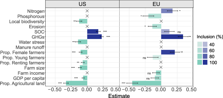
Figure 2. Direction of estimates and effect size of the selected multi-state models and inclusion of each variable in all 1000 bootstrap replications. Crossed variables were not included in the final models. For full results see appendix  ;**
;** ; ***
; *** .
.
Download figure:
Standard image High-resolution imageIn the EU, average AWS, biodiversity, manure runoff, farm size, and proportion of rented land did not remain in the final model (figure 2, appendix
The US and EU models both had some degree of spatial autocorrelation in the residuals, with Moran's I of 0.16 and 0.15, respectively. However, the indicators remained relatively constant when different spatial modelling methods were used (see appendix
See appendix
4.3. AES allocation patterns in individual-State models
Average model fit in the US was higher for states with highest (mean R2 = 0.57 ± 0.27, see appendix
For the EU MS models, few indicators showed significant associations to AES spending per area (see appendix
5. Discussion
Our results suggest some level of inefficacy of AES in targeting areas with the highest environmental needs under current program designs in the US and the EU. While we found agreement between spending and low SOC and high GHG emissions in both the US and the EU, and spending and N surplus in the EU, our findings suggest a mismatch of payments with other environmental variables, including AWS and local biodiversity loss in the US and soil erosion and P balance in the EU. This partially confirms our hypothesis of a mismatch between AES and environmental need when accounting for socio-economic factors that may moderate allocation. These findings support the growing body of literature advocating for more robust spatial targeting of AES, as well as increased consideration of landscape multi-functionality, synergies and trade-offs in AES allocation (Shortle et al 2012, Galler et al 2015, Zasada et al 2018, Pe'er et al 2020, Seppelt et al 2020).
Selected models for the US and the EU retained many of the original environmental and socio-economic indicator variables, confirming that both AES programs rely on similar underlying principles and utilise comparable funding mechanisms (Baylis et al 2008). However, differences were found in the amount of variance explained by the models, with differences among states accounting for more variation in the US than in the EU. This suggests greater variability in allocation formulas among US states than EU MS. This may be explained by the EU's mandate that 25% of the MS budget must be allocated to AES (EU 2005). The uniformity of AES spending in the EU was also confirmed by the lack of within-MS variation in allocation emerging from the individual-State models. These models may have benefitted from finer resolution AES data; however, data for NUTS3 regions is only available from MS-specific databases and was thus not accessible here.
5.1. Successful AES allocation for environmental goals
Our analyses showed success of both EQIP and EAFRD in targeting areas of high GHGs, reflecting the programs' goals regarding agricultural emissions reduction and carbon sequestration. This alignment was also reflected in the models of North Carolina and Arkansas, large producers of livestock, rice, soybeans, feed grains, and cotton—all strong drivers of agricultural GHGs (EPA 2015, FTM 2016, NASS 2017). Cropland and livestock emissions reduction are fundamental for meeting Paris Climate Agreement of mitigation targets (Reisinger and Clark 2018, Rogelj et al 2018), and our results suggest that AES may be successfully targeting areas of greatest need. Although both programmes showed a positive association with SOC, this was only significant in the US. As improved SOC sequestration and agricultural GHG emissions mitigation are linked (Frank et al 2017), this may be a potential win-win scenario from the same AES measures. These results are promising and warrant further investigation to understand the drivers of this successful targeting, which could be applied to other areas of environmental need.
The EU model illustrated EAFRD's success in targeting areas of greatest N surplus. The EU has been addressing issues of N imbalance since the 1990s with the nitrates directive (EU 1991), and our results indicate that the spatial distribution of AES funding may help further reduce N surplus. In contrast, this match was not mirrored by P surplus, which was negatively associated with AES spending. This result warrants further exploration, as the EU lacks a common P management strategy (Ronchi et al 2019).
5.2. Mismatches of AES allocation and environmental need
More so than successes, clear mismatches of funding and environmental needs emerged from our results, highlighting potential misdirection of AES and gaps in environmental targeting of EQIP and EAFRD. Although indicators of soil erosion, biodiversity loss, water stress, and nutrient management are explicitly featured in AES programs' goals (table 2), both the US and the EU showed mismatches between policy priorities and funding allocation. Soil erosion was negatively associated with AES in the EU, and did not feature in the US model, while the opposite was true for local biodiversity.
In the EU, the discrepancy between funding allocation and soil erosion comports with previous studies highlighting how the lack of a common binding strategy has inhibited soil conservation efforts (Turpin et al 2017, Helming et al 2018), a shortcoming that the new Healthy Soil Initiative strives to mitigate (EC 2020b). Moreover, the absence of an association with biodiversity conforms with existing literature highlighting insufficient spatial targeting of conservation measures (Pe'er et al 2014, Batáry et al 2015). In the EU, 0.57% of EAFRD funding is reserved for Natura 2000 sites (Measure 12, Dwyer et al 2016); however, the agricultural matrix surrounding protected areas is crucial in supporting biodiversity (Gonthier et al 2014) and biodiversity conservation is among the supporting ecosystem services financed within Measure M10 ('Agri-environment climate').
We found that subsidy allocation in the US concentrated in areas of reduced water stress need, while the variable was excluded from the EU model. Agriculture is a major cause of freshwater ecosystems degradation (Allan 2004, Poole et al 2013) and water efficiency is becoming increasingly important in light of climate change and groundwater depletion (Marshall et al 2015, Cotterman et al 2018). Thus, this mismatch warrants further policy attention. While it is possible that high water stress and at-risk biodiversity areas are more likely to be enrolled in the CRP program in the US due to its focus on environmentally sensitive lands, or in complementary initiatives like the Conservation Reserve Enhancement Program, this result also highlights the lack of geographical targeting by EQIP since its 2002 reform (Shortle et al 2012, Drevno 2016, Hellerstein 2017). At the state level, water stress emerged as a strong negative predictor in Oregon, indicating a mismatch between EQIP spending and environmental need. Oregon's water supply is threatened by droughts and irrigation demands, with repercussions for agriculture and public health (OEC 2012, Schimpf and Cude 2020). In the EU, the post-2020 CAP reform revised the water exploitation index to relate water stress to availability of renewable water resources, possibly enabling more efficient AES allocation in the future (EEA, 2020).
Nutrient surplus and runoff, especially when tied with water stress and flooding, have serious socio-environmental repercussions that can be ameliorated with sustainable practices (Jones et al 2017, Blanco-Canqui 2018, Roy et al 2021); however, they did not remain in the US model. As the US accounts for large proportions of global livestock production and cropland N surplus (West et al 2014, FAO 2019b), nutrients are known threats to the US water supply (Grant et al 2002, Howarth et al 2002). EQIP subsidizes nutrient management plans and infrastructure development to improve surface water quality, and mandates 50% of total spending to livestock producers (NRCS 2017). Notably, it provides waste management assistance to concentrated animal feeding operations, leading sources of nonpoint water pollution due to chemical inputs and manure runoff from animal feed crops (Burkholder et al 2007, Martin et al 2018). While conservation practices have been shown to reduce nonpoint source loadings locally (Poudel 2016, Liu et al 2018, Sneeringer et al 2018), significant amounts of agricultural land are over-fertilised and need improved nutrient management (Jackson et al 2000, NRCS 2011, 2013, 2014a, Long et al 2018). Moreover, these 'pay-the-polluter' initiatives have been criticised due to insufficient resources, as well as their full reliance on voluntary compliance (Collins 2012, Shortle et al 2012, Shortle and Uetake 2015, Drevno 2016). It should be noted that demand for EQIP funding consistently exceeds allocation (Stubbs 2010), thus, funding limitations may constrain AES' ability to optimize spatial targeting; our results highlight a potential gap in AES targeting which should be further investigated, particularly due to the severe impacts of nutrient surplus and manure runoff associated with US high livestock densities.
5.3. AES allocation and socio-economic variables
In some cases, social context may explain the mismatch between funding and environmental need. In the EU, AES were allocated to areas with higher proportions of female producers, suggesting that EAFRD program goals regarding gender equality and rural development successfully influenced funding allocation, despite, or perhaps in competition with, environmental need. In the US, instead, the proportion of female producers was negatively associated with county spending. This could be due to gender inequality not being a main focus of EQIP per se, but only of overarching USDA policies (NRCS 2019). There may be opportunities for EQIP to learn from EAFRD's focus on social inclusion, especially considering the propensity of women farmers to farm in sustainable, conservation-oriented ways in line with AES program goals (Paul and Fremstad 2016).
Neither program was successful at targeting younger farmers, although only the EU includes additional benefits for young farmers in policy targets (table 2). This supports the findings from an EU audit that despite policy priorities, young farmer participation is declining due to poorly defined interventions and unsatisfactory monitoring systems (ECA 2017). Rented land did not remain in the EU model, and our findings suggest a negative association between tenancy and AES in the US. While Reimer et al (2013) argued that EQIP funding may be preferred over CRP in states with larger proportions of rented land, other studies indicated land ownership as a positive predictor of EQIP participation at local scales (Parker et al 2007, Nyaupane et al 2012, Zhong et al 2016). Rented land is not an explicit target of either AES program; however, previous studies have evidenced lower uptake of sustainable practices by tenant farmers, particularly in conventional systems (Sklenicka et al 2015, Walmsley and Sklenička 2017, Ranjan et al 2019). Local EQIP initiatives and selected EAFRD measures could thus be tailored towards tenants to increase widespread adoption of sustainable practices in conventional landscapes.
Given EAFRD's re-distributive goals, it is somewhat surprising that farm income was not significantly associated with AES allocation in the EU, although a negative association did exist. This could be due to our focus on measures M4 ('Investments in physical assets') and M10 ('Agri-environment-climate'), while excluding other EAFRD funds. Furthermore, there are myriads of drivers which could motivate farmer AES applications that we do not capture here, including personal beliefs, previous experiences and crop prices (McCracken et al 2015, Pavlis et al 2016, Holland et al 2020). Without detailed information on the applications received and approved, we cannot isolate drivers of farmer adoption from those of EQIP and EAFRD's selection criteria when interpreting socio-economic patterns of AES allocation.
5.4. Influence of farming context on AES allocation
Contextual factors related to agricultural production systems may also explain mismatches between AES spending and environmental need, as previous studies have suggested that production system type and structure are a larger driver of subsidy allocation than environmental conditions (Reimer et al 2013, Reimer and Prokopy 2014, Zasada et al 2018). Our findings suggest that the potential for AES to remediate environmental issues may be curtailed within policy frameworks by limited participation from farmers engaged in highly intensive and expansive operations. This may be due to higher utilisation costs of certain conservation practices in intensive farming, or a greater predisposition for these practices in lower intensity areas (see Früh-Müller et al 2019). This was evidenced by significant negative associations with the proportion of agricultural land cover in the US and EU, and with farm size in the US. In the US, AES spending per area was strikingly lower in central regions typically dominated by large farms, while coastal areas had higher spending, despite being less dominated by agriculture. Similarly, in the EU, predominantly agricultural regions such as central Germany and France received lower payments per area.
Our results align with Zasada et al (2018), who also found that smaller farms were more likely to receive higher AES in the EU. However, previous research on the influence of farm size on US conservation practice adoption reports contrasting results, with some finding larger farms more (Baradi 2009) and other less (McLean-Meyinsse et al 1994) likely to adopt conservation practices. Others assert that the influence of farm size varies depending on the management practice and conservation program in question (Soule et al 2000, Lambert et al 2007, Reimer 2015). Future research should further explore whether these farms are less likely to engage with AES—particularly since they are drivers of sustainability issues and experience environmental risks that AES may help mitigate.
6. Conclusions
Our analysis is novel in its approach to compare subsidy systems across continents using an interdisciplinary, human-environment systems perspective. The differences between US and EU AES systems are well documented; however, by developing a consistent framework to assess environmental need, we have identified successes and mismatches in subsidies allocation, and common challenges and opportunities for future policy development and research in both the US and the EU. These findings can help inform refinements to EQIP and EAFRD allocation mechanisms and identify opportunities for improved spatial targeting of AES spending. Furthermore, we identify several socio-economic factors associated with AES allocation that bear further investigation, including the relationship between production system and likelihood of applying for and receiving payments. Finer-scale analyses could assess further indicators of particular interest for the US or the EU, which we did not include for comparability—for example, demographic indicators to account for underserved producers, including racial minorities and farmers with income at or below the national poverty level in the US, and traditional farmers in the EU. Moreover, we did not account for environmental and socio-economic climate change risks in this analysis, a critical area for the sector, and a strong opportunity for future research. Finally, although we investigate spatial targeting of subsidies, we did not analyse the temporal impact of AES. Long-term maintenance of conservation practices is critical to ameliorate the negative externalities of agriculture. For example, changes in soil carbon can take decades to manifest. Additionally, historical AES payments may show varying associations to environmental needs, due to changes in policy frameworks and allocation formulas that have occurred in recent decades.
This research contributes to the growing evidence-base surrounding spatial targeting of AES programs, with implications for farmer engagement and environmental quality. Identifying mismatches in allocation is particularly relevant in light of recent and upcoming reforms of both subsidy programs. While EQIP is increasing its focus on addressing soil health and climate resilience, biodiversity loss, nutrient management, and water stress warrant further attention. Similarly, as the CAP 2020 reform recognises the need for fundamental approaches to sustainable agricultural management, we identified loss of biodiversity, P surplus, and water stress as EAFRD sustainability goals that may need additional targeting.
Acknowledgments
This paper is the outcome of the ARAGOG ('An area of conflict: the effects of agricultural subsidization on conservation goals worldwide') programme. This work was supported by the National Socio-Environmental Synthesis Center (SESYNC) under funding received from the National Science Foundation DBI-1639145 and by the Helmholtz Research School for Ecosystem Services under Changing Land Use and Climate (ESCALATE, VH-KO-613). GZ acknowledges the support of the BESTMAP project funded by the European Union's Horizon 2020 research and innovation programme under Grant Agreement No. 817501. DES was supported by NRT-INFEWS: UMD Global STEWARDS (STEM Training at the Nexus of Energy, WAter Reuse and FooD Systems), NSF Grant Number 1828910. The authors thank the Environmental Working Group for generously sharing the EQIP data for the US. In addition, the authors thank Bridget Kerner, Zora van Leeuwen, and Tim Winter for discussion during the early stages of the research, Jonathan Kramer for his leadership, and two anonymous reviewers for helpful comments on previous versions of this paper.
Data availability statement
The data that support the findings of this study are available upon reasonable request from the authors.
Contribution
All authors conceptualized the study and collaboratively defined the methodology. S B led analysis and data curation with support from L E, R T, B C, K T. S B, L E, K T, B C led code development process. S B, R T, B C, E S led manuscript writing, with support from L E, N M, M O, D E S, H W and review from M B, R S, G Z. M B, N M, R S, G Z, S B, R T provided project administration support including co-organizing workshops to advance the study. M B, N M, R S, G Z acquired funding to support the work.
Appendix A.: Brief overview of funding allocation mechanisms
A.1. EQIP
Allocation is administered by the USDA's Natural Resource Conservation Service (NRCS), distributed from the federal government to each state first, and then distributed within each state to its counties. For the national allocation to states, NRCS determines each state's EQIP funds using a formula that reflects national priorities and available natural resources, including: the significance of environmental and natural resource concerns and the opportunity for environmental improvement, the ways the program can best assist producers in complying with Federal, State, local, and Tribal environmental laws, and the amount of agricultural land in different land use categories. For state-level fund distribution, the State Conservationist develops an allocation formula, considering State and local level resource concerns, science-based information on environmental status, and relevant local programs and specialized farming operations (e.g. specialty crops, livestock, organic, small-scale), among other factors (NRCS 2019). The incentives provided include technical assistance and cost-shares of up to 75% of implementation costs.
A.2. EAFRD
Funds are provided in the form of less favoured area payments, agri-environment schemes, and investment support towards rural development in MS. The framework for fund allocation is based on a two-tier process: at the central stage (EU level), the overall framework is established, financial modalities are outlined and eligibility criteria are defined. Additionally, the EU outlines a set of six priority areas, including fostering knowledge transfer and innovation; enhancing viability and competitiveness of agriculture; promoting food chain organization, animal welfare and risk management; promoting resource efficiency, and low-carbon and climate resilient agriculture; preserving and enhancing ecosystems; and promoting social inclusion, poverty reduction, and economic development in rural areas. The distribution of the overall amount for rural development between MS is based on objective criteria and past performance. At the second level, MS develop national strategic plans and set quantitative objectives for priority areas. At least four of these national level priorities must address the EU level priorities. A minimum value of 30% of rural development funds must be set aside for environmental management measures, falling primarily within the measures considered in this study: M4 'Investments in physical assets', which receives the highest share of EAFRD budget (24%), and M10 ('Agri-Environment Climate'), which receives the third highest share (20%, ENRD CP 2015). There are several AESs across different EU MS, and the allocation mechanisms for specific subsidies tend to vary depending on the focus of the scheme (EC 2013).
Appendix B.: Brief overview of the conservation reserve program
Administered by the USDA's Farm Service Agency (FSA), the CRP is a land retirement program. In exchange for a yearly rental payment for 10–15 years, farmers enrolled in the program agree to remove environmentally sensitive land from agricultural production and plant species that will improve environmental health and quality (Hellerstein 2017). The long-term goal of the program is to re-establish valuable land cover to help improve water quality, prevent soil erosion, and reduce loss of wildlife habitat. The main mechanism of farmer enrolment in this program is through a competitive process known as CRP General Sign-up. During a bidding period, any farmer with highly erodible or environmentally sensitive cropland can apply for the program by indicating the parcels they wish to enrol and the annual payments they require together with the contract length. FSA then determines allocation based on national rankings of an Environmental Benefits Index (EBI) score and based on an overall budget that varies year by year. All parcels with an EBI score above the critical national cutoff are accepted while all parcels with an EBI score below the cutoff are rejected (Hellerstein 2017). Because CRP is largely a land retirement program, and because of its distinctly bottom-up funding allocation mechanism and decision-making process, this program is fundamentally different from the focus of our study—conservation practices used on working farmland supported by EQIP and EAFRD with largely top-down allocation strategies.
Appendix C.: Manure nitrogen runoff vulnerability index
For each county, the index was calculated following Kellogg (2000):
Surface runoff is a measure of the potential for water soluble nutrients to run off fields during precipitations and flooding. Thus, the index estimates the maximum potential for livestock manure nitrogen to move from farms to the water supply. We estimated the amount of nitrogen excreted by each livestock type following the nitrate vulnerable zones guidance (DEFRA 2013, 2019).
| Livestock type | Total N produced by 1 livestock unit (kg N year−1) |
|---|---|
| Adult bovine | 101 |
| Adult swine | 88 |
| Sheep | 7.6 |
| Goat | 15 |
| Poultry | 231 |
Appendix D.: Maps of predictors used in the analysis
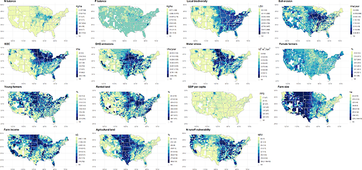
Figure D1. Maps of the predictors used in this study for 48 US states.
Download figure:
Standard image High-resolution image
Figure D2. Maps of the predictors used in this study for 23 EU member states and the UK.
Download figure:
Standard image High-resolution imageAppendix E.: Multi-state models results
Table E1. Regression coefficients of the selected multi-State models in the US and EU and inclusion of each variable in all 1000 bootstrap replications and the frequency of the same direction of the effect in the selected model and the bootstrap replications. * ; **
; ** ; ***
; *** .
.
| US | EU | |||||||||
|---|---|---|---|---|---|---|---|---|---|---|
| Indicator | Estimate | SE | Sig. | Inclusion | Direction | Estimate | SE | Sig. | Inclusion | Direction |
| Intercept | 1.27 | 0.15 | *** | 100.0 | 100.0 | 2.57 | 0.12 | *** | 100.0 | 100.0 |
| Environmental | ||||||||||
| Nitrogen balance | 0.18 | 0.08 | * | 66.6 | 99.8 | |||||
| Phosphorous balance | −0.20 | 0.09 | * | 65.0 | 98.8 | |||||
| Local biodiversity | −0.13 | 0.04 | ** | 92.4 | 100.0 | |||||
| Erosion | −0.14 | 0.07 | * | 67.7 | 98.4 | |||||
| Soil organic carbon | 0.17 | 0.03 | *** | 99.9 | 100.0 | 0.13 | 0.08 | ns | 49.9 | 98.8 |
| GHGs emissions | 0.23 | 0.02 | *** | 100.0 | 100.0 | 0.34 | 0.08 | ** | 99.7 | 100.0 |
| Water stress | −0.14 | 0.04 | ** | 98.0 | 100.0 | |||||
| Manure N runoff | ||||||||||
| Socio-economic | ||||||||||
| Prop. female farmers | −0.10 | 0.02 | *** | 99.7 | 100.0 | 0.21 | 0.07 | ** | 94.6 | 100.0 |
| Prop. young farmers | −0.13 | 0.09 | ns | 41.1 | 96.8 | |||||
| Prop. renting farmers | −0.07 | 0.02 | ** | 86.6 | 100.0 | |||||
| Contextual | ||||||||||
| Farm size | −0.11 | 0.02 | *** | 100.0 | 100.0 | |||||
| Farm income | −0.08 | 0.05 | ns | 88.1 | 57.9 | |||||
| GDP | −0.06 | 0.02 | *** | 99.3 | 100.0 | −0.10 | 0.06 | ns | 75.6 | 100.0 |
| Prop. agricultural land | −0.33 | 0.04 | *** | 100.0 | 100.0 | −0.45 | 0.09 | *** | 99.4 | 100.0 |
Appendix F.: Distribution of correlation coefficients with spending
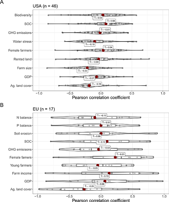
Figure F3. Violin plots of Pearson correlation coefficients between (A) EQIP spending per hectare of agricultural area in the US and (B) EAFRD spending for selected measures per hectare of agricultural area in the EU and the indicator variables. Only correlation coefficients for states and MS with ≥4 regions are shown.
Download figure:
Standard image High-resolution imageAppendix G.: Individual-state models results
Results of the individual-state linear regressions for the selected US states and EU MS. Figure 4 compares direction and estimate size across the US and EU individual-state models. Table 2 shows the estimate model results the ten selected US states, while table 3 shows the estimate model results for the four selected EU MS.

Figure G4. Direction of estimates and effect size in the linear models of individual-state AES allocation in (a) the US states with the greatest and shortest distance from the federal average and (b) the EU for four member states with at least 15 NUTS2-regions. Shaded bars indicate statistical significance with α = 0.05.
Download figure:
Standard image High-resolution imageTable G2. Estimate model results for individual-state analysis in the US for the five states with the greatest and least absolute distance from the average Pearson's correlation coefficient summed across all model variables. * : **
: ** : ***
: *** .
.
| State | Variable | Estimate | SE | t-value | Sig. |
|---|---|---|---|---|---|
| Greatest distance | |||||
| New Mexico (n = 29) R2 = 0.85 | Intercept | 5.71 | 2.20 | 2.59 | * |
| Local biodiversity | −6.68 | 1.34 | −5.00 | *** | |
| Soil organic carbon | 9.63 | 2.43 | 3.96 | *** | |
| GHG emissions | 0.90 | 0.98 | 0.92 | ns | |
| Water stress | 0.97 | 0.65 | 1.49 | ns | |
| Prop. female farmers | −0.03 | 0.13 | −0.21 | ns | |
| Prop. renting farmers | 0.43 | 0.16 | 2.69 | * | |
| Farm size | 0.10 | 0.10 | 0.94 | ns | |
| GDP per capita | −0.19 | 0.12 | −1.58 | ns | |
| Prop. agricultural land | −0.55 | 0.19 | −2.91 | ** | |
| Montana (n = 52) R2 = 0.56 | Intercept | −1.09 | 0.99 | −1.10 | ns |
| Local biodiversity | −0.58 | 0.89 | −0.65 | ns | |
| Soil organic carbon | 1.02 | 0.97 | 1.05 | ns | |
| GHG emissions | −2.85 | 0.98 | −2.90 | ** | |
| Water stress | −0.49 | 0.49 | −1.00 | ns | |
| Prop. female farmers | 0.16 | 0.22 | 0.74 | ns | |
| Prop. renting farmers | 0.62 | 0.22 | 2.78 | ** | |
| Farm size | −0.15 | 0.09 | −1.77 | ns | |
| GDP per capita | −0.12 | 0.14 | −0.85 | ns | |
| Prop. agricultural land | 0.47 | 0.30 | 1.60 | ns | |
| Nebraska (n = 92) R2 = 0.17 | Intercept | 2.12 | 0.70 | 3.01 | ** |
| Local biodiversity | −0.89 | 0.80 | −1.11 | ns | |
| Soil organic carbon | 0.20 | 0.67 | 0.30 | ns | |
| GHG emissions | 0.22 | 0.16 | 1.42 | ns | |
| Water stress | −0.60 | 0.36 | −1.65 | ns | |
| Prop. female farmers | −0.15 | 0.28 | −0.54 | ns | |
| Prop. renting farmers | 0.05 | 0.39 | 0.13 | ns | |
| Farm size | −0.02 | 0.24 | −0.10 | ns | |
| GDP per capita | 0.30 | 0.22 | 1.36 | ns | |
| Prop. agricultural land | −0.35 | 0.53 | −0.65 | ns | |
| Oregon (n = 33) R2 = 0.49 | Intercept | 1.85 | 3.86 | 0.48 | ns |
| Local biodiversity | −7.09 | 4.39 | −1.61 | ns | |
| Soil organic carbon | −1.65 | 2.78 | −0.59 | ns | |
| GHG emissions | 7.26 | 4.37 | 1.66 | ns | |
| Water stress | −14.68 | 5.71 | −2.57 | * | |
| Prop. female farmers | −0.90 | 1.28 | −0.71 | ns | |
| Prop. renting farmers | 0.61 | 0.94 | 0.65 | ns | |
| Farm size | −1.36 | 1.01 | −1.34 | ns | |
| GDP per capita | 0.50 | 0.36 | 1.38 | ns | |
| Prop. agricultural land | −0.14 | 1.34 | −0.10 | ns | |
| Wyoming (n = 21) R2 = 0.61 | Intercept | −4.99 | 3.17 | −1.57 | ns |
| Local biodiversity | −2.44 | 3.94 | −0.62 | ns | |
| Soil organic carbon | 6.59 | 5.23 | 1.26 | ns | |
| GHG emissions | 3.69 | 3.69 | 1.00 | ns | |
| Water stress | −3.31 | 1.42 | −2.33 | * | |
| Prop. female farmers | −0.61 | 0.50 | −1.20 | ns | |
| Prop. renting farmers | −1.04 | 0.41 | −2.53 | * | |
| Farm size | −0.28 | 0.16 | −1.73 | ns | |
| GDP per capita | 0.03 | 0.20 | 0.14 | ns | |
| Prop. agricultural land | −0.95 | 0.73 | −1.31 | ns | |
| Least distance | |||||
| Arkansas (n = 75) R2 = 0.14 | Intercept | 0.85 | 4.68 | 0.18 | ns |
| Local biodiversity | −1.06 | 3.80 | −0.28 | ns | |
| Soil organic carbon | 2.22 | 7.50 | 0.30 | ns | |
| GHG emissions | 2.64 | 1.24 | 2.12 | * | |
| Water stress | −3.17 | 4.27 | −0.74 | ns | |
| Prop. female farmers | −1.61 | 1.93 | −0.83 | ns | |
| Prop. renting farmers | −1.35 | 1.74 | −0.78 | ns | |
| Farm size | −4.13 | 5.25 | −0.79 | ns | |
| GDP per capita | −1.02 | 1.28 | −0.80 | ns | |
| Prop. Agricultural land | −2.22 | 4.62 | −0.48 | ns | |
| Idaho (n = 40) R2 = 0.14 | Intercept | 4.54 | 1.72 | 2.65 | * |
| Local biodiversity | −5.68 | 4.44 | −1.28 | ns | |
| Soil organic carbon | 0.36 | 1.94 | 0.19 | ns | |
| GHG emissions | −0.32 | 0.76 | −0.41 | ns | |
| Water stress | −4.43 | 4.50 | −0.98 | ns | |
| Prop. female farmers | −0.76 | 1.02 | −0.74 | ns | |
| Prop. renting farmers | −0.13 | 0.78 | −0.17 | ns | |
| Farm size | −0.02 | 1.82 | −0.01 | ns | |
| GDP per capita | −1.41 | 1.03 | −1.38 | ns | |
| Prop. Agricultural land | −1.85 | 1.68 | −1.10 | ns | |
| North Carolina (n = 92) R2 = 0.13 | Intercept | −0.10 | 3.94 | −0.03 | ns |
| Local biodiversity | 1.51 | 3.27 | 0.46 | ns | |
| Soil organic carbon | 0.55 | 1.06 | 0.52 | ns | |
| GHG emissions | 1.88 | 0.62 | 3.03 | ** | |
| Water stress | −1.35 | 3.09 | −0.44 | ns | |
| Prop. female farmers | 0.43 | 0.89 | 0.48 | ns | |
| Prop. renting farmers | 0.91 | 1.01 | 0.90 | ns | |
| Farm size | −11.20 | 6.38 | −1.76 | ns | |
| GDP per capita | −2.21 | 0.97 | −2.27 | * | |
| Prop. Agricultural land | −2.67 | 3.35 | −0.80 | ns | |
| Oklahoma (n = 77) R2 = 0.20 | Intercept | 1.43 | 0.51 | 2.80 | ** |
| Local biodiversity | −1.92 | 0.66 | −2.90 | ** | |
| Soil organic carbon | 2.11 | 0.80 | 2.64 | * | |
| GHG emissions | 0.66 | 0.39 | 1.67 | ns | |
| Water stress | −0.65 | 0.40 | −1.63 | ns | |
| Prop. female farmers | −0.24 | 0.34 | −0.70 | ns | |
| Prop. renting farmers | 0.50 | 0.32 | 1.57 | ns | |
| Farm size | 0.18 | 0.71 | 0.26 | ns | |
| GDP per capita | −0.23 | 0.19 | −1.21 | ns | |
| Prop. Agricultural land | −0.14 | 0.40 | −0.34 | ns | |
| Tennessee (n = 93) R2 = 0.15 | Intercept | 2.13 | 1.73 | 1.23 | ns |
| Local biodiversity | −1.61 | 1.54 | −1.05 | ns | |
| Soil organic carbon | 2.67 | 2.29 | 1.17 | ns | |
| GHG emissions | 1.98 | 1.20 | 1.65 | ns | |
| Water stress | −0.94 | 1.95 | −0.48 | ns | |
| Prop. female farmers | −1.70 | 0.97 | −1.75 | ns | |
| Prop. renting farmers | −1.28 | 0.96 | −1.33 | ns | |
| Farm size | 3.03 | 4.00 | 0.76 | ns | |
| GDP per capita | −0.14 | 0.64 | −0.22 | ns | |
| Prop. Agricultural land | −1.42 | 1.70 | −0.84 | ns | |
Table G3. Estimate model results for individual-State analysis in the EU for the member states with more than 15 NUTS2. * : **
: ** :***
:*** .
.
| Member state | Variable | Estimate | SE | t-value | Sig. |
|---|---|---|---|---|---|
| United Kingdom (n = 31) R2 = 0.81 | Intercept | 74.24 | 31.63 | 2.35 | * |
| Phosphorous balance | −28.18 | 20.96 | −1.35 | ns | |
| Nitrogen balance | −16.87 | 16.11 | −1.05 | ns | |
| Soil erosion | 8.34 | 12.29 | 0.68 | ns | |
| Soil organic carbon | 14.37 | 9.81 | 1.47 | ns | |
| GHG emissions | 40.39 | 19.42 | 2.08 | ns | |
| Prop. of female farmers | −8.64 | 17.63 | −0.49 | ns | |
| Prop. of young farmers | −20.85 | 19.21 | −1.09 | ns | |
| Farm income | −5.24 | 13.75 | −0.38 | ns | |
| GDP per capita | −0.09 | 9.46 | −0.01 | ns | |
| Prop. agricultural land | −53.20 | 9.58 | −5.55 | *** | |
| France (n = 21) R2 = 0.74 | Intercept | 6.94 | 2.67 | 2.60 | * |
| Phosphorous balance | 4.30 | 2.24 | 1.92 | ns | |
| Nitrogen balance | −1.30 | 1.40 | −0.93 | ns | |
| Soil erosion | −0.23 | 1.86 | −0.13 | ns | |
| Soil organic carbon | 0.19 | 2.08 | 0.09 | ns | |
| GHG emissions | −0.64 | 2.60 | −0.25 | ns | |
| Prop. of female farmers | −1.90 | 1.82 | −1.05 | ns | |
| Prop. of young farmers | 0.07 | 2.00 | 0.04 | ns | |
| Farm income | 13.55 | 4.29 | 3.16 | * | |
| GDP per capita | −1.66 | 1.32 | −1.26 | ns | |
| Prop. agricultural land | 3.60 | 2.47 | 1.46 | ns | |
| Italy (n = 19) R2 = 0.64 | Intercept | 87.53 | 101.06 | 0.87 | ns |
| Phosphorous balance | −107.21 | 87.54 | −1.23 | ns | |
| Nitrogen balance | 84.46 | 83.71 | 1.01 | ns | |
| Soil erosion | −0.03 | 10.13 | 0.00 | ns | |
| Soil organic carbon | 87.56 | 105.45 | 0.83 | ns | |
| GHG emissions | 46.50 | 36.99 | 1.26 | ns | |
| Prop. of female farmers | 46.12 | 36.30 | 1.27 | ns | |
| Prop. of young farmers | 52.18 | 28.67 | 1.82 | ns | |
| Farm income | 28.36 | 185.64 | 0.15 | ns | |
| GDP per capita | −6.06 | 30.49 | −0.20 | ns | |
| Prop. agricultural land | 23.33 | 36.64 | 0.64 | ns | |
| Germany (n = 34) R2 = 0.42 | Intercept | 23.97 | 15.05 | 1.59 | ns |
| Phosphorous balance | 6.33 | 5.57 | 1.14 | ns | |
| Nitrogen balance | −5.21 | 5.60 | −0.93 | ns | |
| Soil erosion | 14.96 | 17.92 | 0.84 | ns | |
| Soil organic carbon | 4.41 | 6.45 | 0.68 | ns | |
| GHG emissions | −1.04 | 8.21 | −0.13 | ns | |
| Prop. of female farmers | −4.16 | 12.00 | −0.35 | ns | |
| Prop. of young farmers | −2.60 | 5.91 | −0.44 | ns | |
| Farm income | 7.60 | 6.46 | 1.18 | ns | |
| GDP per capita | −5.98 | 4.64 | −1.29 | ns | |
| Prop. agricultural land | 6.79 | 9.54 | 0.71 | ns |
Appendix H.: Spatial models
We used Moran's I statistic to determine the relationship between the US and EU model residuals and their surrounding values. We tested this with a Monte-Carlo simulation with 1000 permutations using moran.mc in the spdep R package. This compares the observed value of Moran's I with a simulated distribution to assess the likelihood that the observed values could be observed at random. We tested several spatial models on our data, and present the spatial error models obtained with errorsarlm from the spatialreg package in R.
The US model had a Moran's I of 0.16 indicating that there was some spatial autocorrelation in the residuals. There was a correlation of each county and the adjacent counties of 0.31, and the random intercepts for each state revealed a pattern of coastal states having positive random intercepts. Figure H5 shows the residuals of the model, and figure H6 the random intercepts. Table H4 and figure H7 present the spatial error model.

Figure H5. Residuals of the US model by county.
Download figure:
Standard image High-resolution image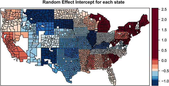
Figure H6. Random intercepts of the US model by state.
Download figure:
Standard image High-resolution image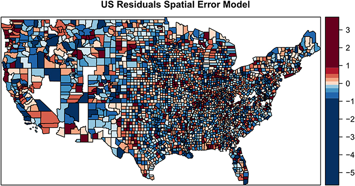
Figure H7. Residuals of the spatial error model by county.
Download figure:
Standard image High-resolution imageTable H4. Spatial error model for the US. * ;**
;** ; ***
; *** .
.
| Variable | Estimate | SE | z-value | Sig. |
|---|---|---|---|---|
| Intercept | 1.123 | 0.14 | 7.993 | *** |
| Local biodiversity | −0.097 | 0.05 | −2.004 | * |
| Soil organic carbon | 0.164 | 0.04 | 4.423 | *** |
| GHG emissions | 0.253 | 0.03 | 9.636 | *** |
| Water stress | −0.107 | 0.05 | −2.344 | * |
| Prop. female farmers | −0.069 | 0.02 | −2.928 | ** |
| Renting farmers | −0.068 | 0.02 | −2.878 | ** |
| Farm size | −0.111 | 0.03 | −4.367 | *** |
| GDP per capita | −0.06 | 0.02 | −3.678 | *** |
| Prop. agricultural land | −0.318 | 0.04 | −7.906 | *** |
The EU model also had a Moran's I of 0.15. The random intercepts did not show a clear geographic pattern, however, there was a correlation of each NUTS2 region and the adjacent regions of 0.26. Figure H8 shows the residuals at NUTS2 level, figure H9 the random intercept for each country, and table H5 the spatial error model output shown in figure H10.
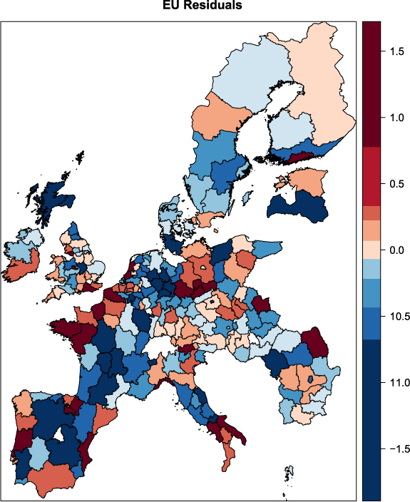
Figure H8. Residuals of the EU model by NUTS2.
Download figure:
Standard image High-resolution image
Figure H9. Random intercepts of the EU model by member State.
Download figure:
Standard image High-resolution image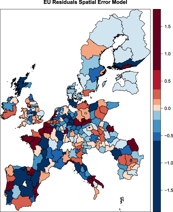
Figure H10. Residuals of the EU spatial error model by NUTS2.
Download figure:
Standard image High-resolution image
Table H5. Spatial error model for the EU.  ;**
;** ; ***
; *** .
.
| Variable | Estimate | SE | z-value | Sig. |
|---|---|---|---|---|
| Intercept | 2.751 | 0.339 | 8.113 | *** |
| Nitrogen balance | 0.166 | 0.081 | 2.062 | * |
| Phosphorous balance | −0.173 | 0.084 | −2.051 | * |
| Soil erosion | −0.142 | 0.062 | −2.302 | * |
| Soil organic carbon | 0.197 | 0.082 | 2.401 | * |
| GHG emissions | 0.313 | 0.077 | 4.046 | *** |
| Prop. of female farmers | 0.258 | 0.084 | 3.056 | ** |
| Prop. of young farmers | 0.001 | 0.104 | 0.007 | ns |
| Farm income | −0.127 | 0.048 | −2.631 | ** |
| GDP per capita | −0.097 | 0.061 | −1.592 | ns |
| Prop. agricultural land | −0.487 | 0.089 | −5.449 | *** |