


Abstract
There is much current debate about the way in which the earth's climate and temperature are responding to anthropogenic and natural forcing. In this paper we re-assess the current evidence at the globally averaged level by adopting a generic 'data-based mechanistic' modelling strategy that incorporates statistically efficient parameter estimation. This identifies a low order, differential equation model that explains how the global average surface temperature variation responds to the influences of total radiative forcing (TRF). The model response includes a novel, stochastic oscillatory component with a period of about 55 years (range 51.6–60 years) that appears to be associated with heat energy interchange between the atmosphere and the ocean. These 'quasi-cycle' oscillations, which account for the observed pauses in global temperature increase around 1880, 1940 and 2001, appear to be related to ocean dynamic responses, particularly the Atlantic multidecadal oscillation. The model explains 90% of the variance in the global average surface temperature anomaly and yields estimates of the equilibrium climate sensitivity (ECS) (2.29 ∘C with 5%–95% range 2.11 ∘C to 2.49 ∘C) and the transient climate response (TCR) (1.56 ∘C with 5%–95% range 1.43 ∘C to 1.68 ∘C), both of which are smaller than most previous estimates. When a high level of uncertainty in the TRF is taken into account, the ECS and TCR estimates are unchanged but the ranges are increased to 1.43 ∘C to 3.14 ∘C and 0.99 ∘C to 2.16 ∘C, respectively.
Export citation and abstract BibTeX RIS

Original content from this work may be used under the terms of the Creative Commons Attribution 4.0 license. Any further distribution of this work must maintain attribution to the author(s) and the title of the work, journal citation and DOI.
1. Introduction
The rapidity of the change in global average surface temperature anomaly (GTA) and the levels that this will reach are still in doubt, partly because of uncertainty about the actions that will be taken to alleviate the anthropogenic causes of warming; and partly because of the uncertainty associated with the models used to evaluate the dynamic relationship between the radiative forcing and the GTA. The ultimate global temperature equilibrium response to a doubling of the atmospheric CO2 concentration above its pre-industrial concentration (generally taken to be  [1]) or equilibrium climate sensitivity (ECS), is one of the main climatic measures of future warming potential [2, 3]. The transient climate response (TCR) is a more immediate measure of global temperature change, defined as the temperature increase at the instant the atmospheric CO2 has doubled, following a increase of 1% each year compounded to give a doubling time of 70 years. In contrast to the ECS, which is precisely defined in terms of the estimated model parameters (see later, section 2), the TCR is more subjective, appearing to derive from assumptions made by Wanabe et al [4] in 1991.
In a recent assessment of the ECS using a form of the Hasselman model, with an auto-regressive emergent constraint, Cox et al [3] report an ECS of 2.8 ∘C with 66% confidence limits of 2.2 ∘C–3.4 ∘C (see also [5]). Such a large uncertainty range can make IPCC policy planning based on them rather challenging and can inhibit our ability to establish predictive capacity for this climate system. Calculations based on historical data give rise to smaller values of ECS than Atmosphere-Ocean General Circulation Models (AOGCMs) or paleoclimate data. For example, the review by Knutti et al [6] reports that observationally-based estimates of ECS (mean 2.51 ∘C) are notably lower than estimates from AOGCMs and paleoclimatology data (mean 3.41 ∘C). Current very likely estimates for TCR fall in the range of 1 ∘C–2.3 ∘C with mean of 1.7 recently established with emergent constraint methods [5]. The mean TCR for 25 observationally-based studies reported in Knutti et al [7] is 1.51 ∘C and the 5% and 95% limits of their distribution are 0.91–2.11. This range is also representative of those individual studies for which 5% and 95% limits are recorded. Possible biases in the estimates obtained by these various approaches are discussed briefly in section 5.
1.1. Data-based mechanistic (DBM) modelling
The approach to estimating the ECS and TCR values used in the present paper is quite different from the methods mentioned above. It is based on previous research (see e.g. [2, 8–12]) that shows how models of low dynamic order are able to both emulate very closely the behaviour of large climate simulation models, at the globally-averaged level, and explain the historical, globally averaged climate data. In both cases, the estimated model parameters can then provide estimates of the associated climate parameters. This approach exploits a method of dynamic systems analysis known as DBM modelling (see e.g. [13–15] and the prior references therein). This is a general, statistically-based modelling approach that was originally developed in a dynamic systems and control setting and applied in hydrology, where it is now one of the standard approaches to modelling rainfall-flow behaviour [16]. It has been developed and used successfully for applications in other areas of study, from ecology and engineering to macro-economics (see [13]), as well as climate (see e.g. [9, 17, 18]).
The DBM modelling approach employs statistically efficient methods of time-series model estimation for continuous-time differential models and is designed specifically to identify those physically meaningful dynamic properties of a dynamic system that are identifiable from time-series data. Such differential equation models have a number of advantages, from both scientific and statistical standpoints [19]. In the context of climate system modelling, they are of the same general, differential equation form as those used in the construction of global climate models, but with a dynamic order identified objectively from the globally averaged data to capture the identifiable 'dominant modes' [20] of the observed dynamic behaviour in the globally averaged system. Most importantly, the main equation in the DBM model identified in this paper is characterized by parameters that have immediate physical meaning within the global dynamic system and, as we will see, it can be compared directly with simple energy-balance models of the climate system. Finally, the model accommodates and quantifies the stochastic nature of the dynamic system, so that the resulting uncertainty bounds estimated for ECS and TCR are easily evaluated and based on the information that is intrinsic to the data record. Although it has these advantages, DBM modelling is an approach that has not been widely deployed in ECS assessment to date, and so the results presented in the paper provide fresh insight into the value of these parameters and the related mechanisms on which they depend.
1.2. Globally averaged climate data
The data used for DBM modelling in this paper are the annual, globally averaged climate data, shown in figure 1 for the historical period from 1856 to 2015. The GTA in figure 1(a) represents the changes in the globally averaged surface temperature around a level defined by the average of the temperature measurements over the period 1951–1980. The total radiative forcing (TRF) in figure 1(b) is the sum of radiative forcing components due to: CO2 in the atmosphere; volcanic activity; solar variability; and all other anthropogenic sources (including negative forcing from aerosols and indirect effects). Taking year 2005 as illustrative (all values in W m−2), the TRF = 2.08 which, when solar and volcanic forcings are subtracted, yields a total anthropogenic forcing of 1.84, made up of:
- Greenhouse gases, Kyoto and Montreal protocol minor gases = 2.65,
- Direct aerosols (organic and black carbon, SOx, NOx, biomass burning, mineral clouds) = −0.41, and
- Miscellaneous forcings (cloud albedo, stratospheric and tropospheric ozone, methane oxidation, changes in land use and black carbon on snow) = −0.39.
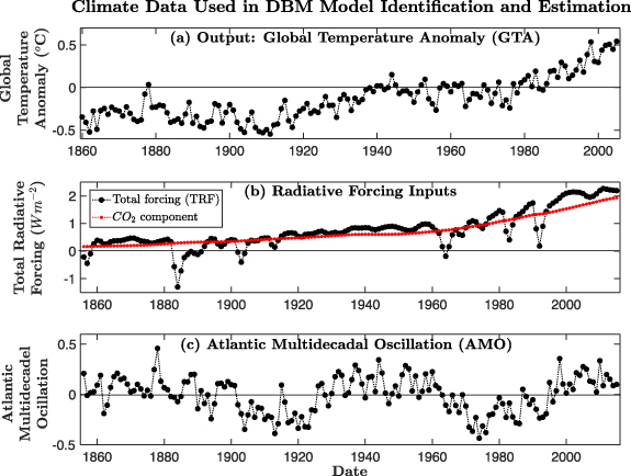
Figure 1. Global climate data: (a) GTA measurements, from the Carbon Dioxide Information Analysis Center (CDIAC); (b) the TRF signal and the CO2 component of this total signal, from the Potsdam Institute for Climate Impact Research website; (c) the AMO series, downloaded from the Physical Sciences Division, Earth System Research Laboratory of NOAA.
Download figure:
Standard image High-resolution imageAs we see later, the sharp negative excursions are associated with volcanic eruptions that are not always considered in climate modelling studies (see e.g. figure SPM.5 in the IPCC 5th Assessment Report) but prove useful in establishing both the identifiability and novel structural nature of the DBM model. The physical mechanisms that affect the relationship between the TRF and the GTA are inferred from the constant-parameter DBM model identified from the data in figure 1. As discussed in the next section 2, the main climatically meaningful parameters derived from the model parameter estimates are the ECS; the effective heat capacity of the ocean (EHC); the TCR; and the feedback response time (FRT or 'Time Constant'), Tc .
2. Estimation of global climate parameters from observations
Climate modelling normally starts from basic physical principles, where the standard differential equation for heat balance is [21]:
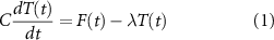
in which T(t) is the GTA and F(t) is the TRF. Forcing inputs are offset by various feedbacks, linearly approximated by λT(t), the climate feedback parameter multiplied by surface temperature anomaly. The out-of-equilibrium imbalance is measured by the heat flux into the ocean, ice and land [6] as  , where C is a constant EHC per unit area [22–24]. The rapid and slow thermal response of the oceans is part of this dynamic behaviour. For the subsequent analysis, it helps to write equation (1) in the following form:
where x(t) = T(t) and u(t) = F(t).
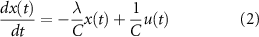
The DBM approach to modelling the energy balance is quite different because the differential equation model structure is identified directly and objectively from the time series data using model order identification criteria (see chapter 6 in [13]) to ensure that the model is not over-parameterized and is fully identifiable from the available data. The parameters associated with this identified model structure are then estimated using maximum likelihood optimization. In this case, the resulting DBM model takes the following form:
Here u(t − τ) is the TRF delayed by τ years that acts as an the input to the second differential equation in the variable x2(t); and x(t) is the simulated deterministic output of the model which simply combines the outputs of the two component equations to produce the model estimate of the GTA.
Although the model (3) is a continuous-time differential equation, the observations related to this are the discrete-time, annually sampled data in figure 1. The associated observation equations are represented as follows:

Here, the argument 'k' indicates the sampling instant with k = 1 : N, where N = 160 is the number of annual samples from 1856 to 2015. The disturbance ξ(k) is identified as 'coloured noise' generated from a zero mean, serially uncorrelated and normally distributed series e(k), with variance σ2, by a first order AutoRegressive (AR) model. Correlation analysis confirms that, as required, the residual series e(k) is both serially uncorrelated in time and uncorrelated with the observed TRF input series u(k), with a zero mean, approximately normal amplitude distribution. It represents the completely random and irreducible source of uncertainty in the model.
The optimal estimates of the parameters in the model equations (3) are obtained using standard DBM analysis (see [25] for full details of the analysis), which yields estimates of  and
and  . The ECS is obtained by multiplying the steady state gain
  by 3.7 W m−2 to yield 2.29 ∘C. The FRT is given by
  years; and the time delay τ = 17.5 years. An estimate of the TCR is obtained by simulating the model with the prescribed input (see section 1), which yields a value of 1.56 ∘C. This is lower than the 1.7 ∘C estimate of Nijsse et al [5] but within their estimated 5%–95% uncertainty range of 1.0 ∘C to 2.3 ∘C. One advantage of the present analysis, in relation to that of Andrews and Allen [21], for example, is that we are able to evaluate the uncertainty in the EHC and λ, or any of the other parameters. The evaluation of uncertainty in climate models is, of course, very important and this is discussed later in section 5.
3. The model response and the dynamic characteristics of x1(t) and x2(t)
Figure 2 shows the GTA response to the TRF input (red line) and the two components x1(t) (dash-dot red line) and x2(t) (black line), generated by the DBM model (3). The red arrows draw attention to where the reductions in x2(t) tend to counteract the increases of x1(t) and lead to the 'leveling' periods in the GTA, the last one starting around 2000.

Figure 2. The output of the final DBM model (red full line) compared with the GTA data. Also shown are the component states x1(t) (red dash-dot line) and x2(t) (black line), which is raised by 0.7 ∘C for clarity.
Download figure:
Standard image High-resolution imageFigure 3 shows the response of the estimated model (3) to a forcing step input of 3.7 W m−2, where the step is applied after 150 years. Note how the oscillations in x2(t) are: (i) decaying slightly as time progresses because there is no further change in the TRF input to excite them; (ii) have a zero mean value because x2(t) oscillates continually with similar positive and negative excursions about x1(t); and (iii) that this does not affect the underlying x1(t) response, nor the final equilibrium level of x(t) and the related estimate of the ECS. This behaviour arises because equation (3)(ii) is a 'stochastic oscillator' which needs sufficient excitation from the TRF to generate and sustain its oscillations. Consequently, a slow ramp-up of the TRF input taking 200 years to go from zero to 3.7 W m−2, without any sharp changes in level, does not excite the oscillator sufficiently for larger oscillations to be generated (red dashed line in figure 3). This means that the volcanic eruptions are required to excite the oscillatory mode and this will not show up in the absence of volcanic effects, as when forecasting or performing scenario analysis, unless such perturbations in the TRF are introduced into these exercises (see section 7 and [25]).
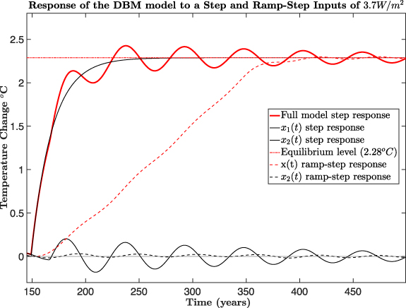
Figure 3. DBM model response to sharp and slow ramp-step changes of 3.7 W m−2 in the TRF input applied after 150 years.
Download figure:
Standard image High-resolution image4. The quasi-cycle oscillations of the state x2(t)
The identification of the oscillatory state x2(t) was not anticipated and shows the value of the DBM approach in uncovering unexpected aspects of the measured dynamic behaviour [25]. The estimated period of the oscillations in x2(t) is Pn = 55.3 years, with a 5%–95% range between 51.6 and 60 years (see section 5). Most significantly in climatic terms, the recession periods of this oscillation coincide with and help to explain the climate shifts ('pauses' or 'leveling') in the generally upward trend of the GTA, as we have seen in figure 2 and which affect the forecasting results, allowing for the prediction of the 'leveling' after 2000 [2]. The importance of an internal multidecadal oscillation mode, its dominance in the Atlantic and its global temperature influence, has also been noted by Knutson et al [26] and Barcikowska et al [27]. The stochastic oscillations and the leveling periods seen in the GTA response of our DBM model are consistent with their conclusions.
The potential importance of quasi-cyclic behaviour with a period of around 50–70 years has been known for some time. For example, Schlesinger and Ramankutty [28] applied singular spectrum analysis to four global-mean temperature records and identified a temperature oscillation with a period of 65–70 years. They conclude that this is the statistical result of 50–88 year oscillations for the North Atlantic Ocean and its bounding Northern Hemisphere continents. Furthermore, Bruun et al [29] and Sk kala et al [30] have shown that such a global pentadecadal model is also a resonance consequence of wave interaction properties at the ocean basin scale. The Atlantic multidecadal oscillation (AMO) variable plotted in the lower panel of figure 1, as well as other multidecadal oscillatory phenomena measured by climate scientists, could be redolent of complex internal energy exchange mechanisms that are giving rise to significant quasi-cyclic behaviour in the ocean-atmosphere system.
We anticipate that these quasi-cyclic phenomena are related to the features represented by the oscillatory state variable x2(t) and the decomposed structure of the equation (3)(ii) that can be obtained using the transfer function (TF) decomposition methods that are well known in systems and control analysis (see [25]). This yields the block diagram shown in figure 4, where the relevant equations are included in the two boxes, rather than the standard TF representations, so that the climatic meaning is clearer to readers previously unacquainted with the TF methods of model analysis. The differential equations of this decomposed model take the form:
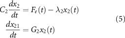
where x21(t) is the 'feedback path' variable and  is the difference between the delayed incoming TRF input and x21(t), which provides the input to the energy balance equation in the forward path (cf equation (1)). This is a negative feedback system where the feedback path consists of a simple integrator with gain G2 that accumulates the changes in the x2(t) component of the GTA. The estimated parameters in this feedback model are
  and G2 = 1.913.

Figure 4. Decomposed negative feedback block diagram of the model for x2(t).
Download figure:
Standard image High-resolution imageThe overall effect of this negative feedback mechanism is to create the oscillatory mode of behaviour that is so important in explaining the subtle oscillatory 'quasi-cycle' variations observed in the GTA. In other words, the combination of the gains and time constants in the two boxes is creating some form of heat energy exchange that promotes the oscillatory nature of the response. The presence of the integrator in the feedback path suggests that this feedback part of the system relates to mixing processes that are very long term. This is consistent with transport processes that occur slowly in the global oceanic system, which is accumulating the effects of the changes in the globally averaged temperature. Thus we can surmise that this interchange of energy between the atmosphere and the ocean, and vice-versa, is a physical process that has helped to sustain the oscillatory movements in x2(t) and so caused fairly regular, periodic changes in the GTA over the last 160 years. The features of the volcanic excitation of the stochastic oscillator we present here could help explain the empirical finding of Canty et al [31], where an attenuated volcanic forcing linkage with AMO and GTA response has been noted, with a periodicity of about 65 years.
Considering the above results, we can be reasonably confident that the oscillatory state is present and playing an important part in explaining the changes in the GTA. Moreover, the decomposition into the feedback system is a standard procedure that produces a unique deterministic result; and the interpretation in this decomposed form, with an integrator in the feedback path, makes reasonable physical sense. On the other hand, while the structure of this decomposition is well defined, the estimated parameters that characterize this structure are quite uncertain (see [25]). As a result, the values of the parameters in the decomposed system, and any interpretation of them, must be considered with some circumspection. Clearly, more research is required to interpret the nature of the heat energy exchanges that are suggested by the decomposed model.
Finally, it is interesting to note the high correlation between the estimated quasi-cycle and the quasi-cycle in the AMO series. Schlesinger and Ramankutty [28] suggest that the most probable cause of the AMO is an inherent internal oscillation of the atmospheric-ocean system. This seems a reasonable argument and so it makes sense to consider how the AMO oscillations can be modelled in a way that links them with the internal oscillatory state x2(t). The full details of this analysis are given in [25] and it will suffice here to say that x2(t) can be related reasonably well to the AMO by a second-order model.
5. Uncertainty and climate modelling
The authors of chapter 1 of the 2019 Special IPCC Report [32] introduce the term 'deep uncertainty' as a situation when experts or stakeholders do not know or cannot agree on: (1) appropriate conceptual models that describe relationships among key driving forces in a system; (2) the probability distributions used to represent uncertainty about key variables and parameters; and/or, (3) how to weigh and value desirable alternative outcomes. They point out that such problems go back at least to the 1979 assessment by the US National Academy of Sciences, commonly referred to as the 'Charney Report'.
One particular problem is the evaluation of uncertainty in the TRF input, where the uncertainty is considered as the sum of the uncertainties of its components, as quantified by the 5 and 95% uncertainty bounds, defined by 'line-by-line' estimates, or ensemble results, obtained from the atmospheric chemistry modules of AOGCMs (as part of the ACCMIP). With AOGCMs, the bounds on the GTA are then evaluated from an ensemble of simulations with, as far as we can ascertain, no attention paid to possible covariance between these uncertainty values. Alternatively, with single equation approaches, such as energy balance models, the associated regression coefficient variance and residual errors are used, sometimes employing a Bayesian approach. However, the currently estimated climate sensitivity values and range obtained in this manner are likely to be affected deleteriously because, by focusing on fast feedbacks, the slowly varying and mostly oceanic component wrongly features as serial correlation in the error processes [32].
In the present paper, uncertainty is handled using an approach that is well known in the statistics, time series analysis and dynamic systems analysis. The estimated uncertainty in the DBM model parameters, as defined by the estimated parametric error covariance matrix, defines the uncertainty in the estimates of the model parameters and provides the required information for the Monte Carlo (MC) simulation analysis used to estimate the climate parameters that are derived from these (see e.g. [13]). The uncertainties in the climatically important derived parameters, as obtained using this analysis, are shown in table 1, based on the Cholesky factorization of the estimated covariance matrix. These figures can be compared with those in table S8.1 of Randall et al [33], as obtained from MAGICC emulations of the 18 AOGCMs used in the CMIP3 and used by Andrews and Allen [34] to calculate time constants. Based on this table, the means and 5%–95% confidence intervals for the ECS and Tc
, respectively, are 2.95 ∘C (2.17 ∘C–3.13 ∘C); and 30.3 years (16.0–44.7 years) and our DBM model results fall within these bounds. Van Hateren [12] is one study in the same spirit as the present one, although with more assumptions and restrictions. His ECS estimate is 2.0 ∘C (1.5 ∘C–2.5 ∘C) and his TCR estimate is 1.5 ∘C (1.2 ∘C–1.8 ∘C). His intervals are widened by about 0.4 ∘C based on uncertainty over the value of forcing for CO2 doubling. Our estimate of EHC is  , with a 5%–95% range of 26.9 to 37.3. This compares with the results of Knutti et al [6], who provide an estimated EHC of
  , and corresponding 5%–95% interval of 6–
 , based on their analysis of 17 CMIP3 GCM models. In the recent wide-ranging ECS sensitivity review and assessments of Sherwood et al [35], they report a baseline ECS 5%–95% range of 2.3 ∘C–4.7 ∘C. Our reported ECS is 2.29 ∘C with 5%–95% range 2.11 ∘C to 2.49 ∘C, which is within their uncertainty range. As in the deterministic case, the MC-based estimate of TCR is obtained by repeated simulation of the DBM model for the prescribed input (see section 1), yielding 1.56 ∘C (with a 5%–95% interval of 1.43 ∘C–1.68 ∘C). This estimate is within the 5%–95% range of 1.0 ∘C–2.3 ∘C recently established with 'Emergent Constraint' methods [5] but the mean is lower than the 1.7 ∘C they obtain.
Table 1. MC simulation results for the Final DBM Model based on 100 000 random realizations defined by the estimated error covariance matrix. When the TRF is treated as a noisy series, the MC simulation is computationally intensive, requiring parameter re-optimization for each draw. However, this leads to results similar to those in this table [25].
| Parameter (units) | Estimate | 5% Bound | 95% Bound |
|---|---|---|---|
| ECS (∘C) | 2.29 | 2.11 | 2.49 |
| TCR (∘C) | 1.56 | 1.43 | 1.68 |
| Tc (y) | 19.3 | 16.5 | 23.3 |
| Pn (y) | 55.3 | 51.6 | 60.0 |
λ ( ) ) | 1.62 | 1.49 | 1.75 |
C ( ) ) | 31.2 | 26.9 | 37.3 |
The narrow uncertainty bounds shown in table 1 arise because the TRF input used in the DBM model analysis is that evaluated over the period 1856–2015, as shown in the middle panel of figure 1, which contains significant effects of volcanic activity that have been excluded from some studies. It is clear, however, that any additional uncertainty in the TRF will lead to increased uncertainty bounds for the parameters in table 1 and this needs to be considered. Using an approach that is well known in the systems literature, this uncertainty in the TRF input could be evaluated by optimal fixed interval smoothing estimation of the time variable parameters in a dynamic harmonic regression (DHR) model; and this is could then used as the stochastic input in the MC simulations. However, this leads to the relatively small level of uncertainty in the TRF shown in the top panel of figure 6, as discussed in the next section 6.
Considering the nature of the TRF components and their methods of measurement, it is not surprising that there is some debate about the TRF and its associated uncertainty. Several explicitly calculated time series of the radiative forcing have appeared in the climate literature over the twentieth century, for example those cited in Schwartz [36]. These data sets are point estimates and cannot be taken together to estimate a distribution of forcing values. The most widely agreed distribution is that appearing in the 2013 IPCC Report [37] and so we base our estimates on the 90% uncertainty range for 2011 that appears in figure SPM.5 on page 14 of the 'Summary for Policy makers', with a lower bound 1.13 W m−2 and an upper bound 3.33 W m−2. This is based on the TRF in 2011 relative to 1750 and so it represents a considerable level of uncertainty if it is applied uniformly over the 160 years of data. In addition, we also take into account the uncertainty on the estimated parameters in table 1, which adds 25% more uncertainty to the radiative forcing. In total, this translates to a total uncertainty range of ±1.38 W m−2 on the TRF input. When this very high level of uncertainty is applied, it naturally leads to considerably revised bounds for the climate parameters estimates in table 1 of 1.43 ∘C–3.14 ∘C for the ECS; and 0.99 ∘C–2.16 ∘C for the TCR.
Marvel et al [38] conclude that ECS estimated from historical Atmospheric Model Intercomparison Project climate model simulations is biased low compared to abrupt 4 × CO2 experiments. However, it is important to note that their estimate is based on simulation data over the fairly short 1979–2005 period and not, as in this paper, on the longer globally averaged historical time series from 1856 to 2015. On the other hand, these historical records are still relatively short and the climate signal is masked by sufficient noise that even optimal statistical estimation is unlikely to be able to extract robust estimates of very low frequency components [25]. However, these contribute little to warming in the early decades of a forcing response.
The evidence for such long period time constants is naturally present in simulation model data but only because these are based, in part, on hypotheses about the long-term behaviour of the climate that will naturally affect the resulting ECS estimate. Our DBM modelling, on the other hand, is concerned only with inferences that can be made from time series that derive from observational data and so it is not influenced by simulation model construction hypotheses. This is not in any way a criticism of large climate model simulations; it is simply to emphasize the difference between analysis based on such simulated data and that based directly on the historical data, as reported in the present paper. We believe that the results from both sources are important in any balanced, model-based assessment of global warming.
Finally, given the importance attached to the ECS in climate change research, it is reasonable to ask whether our estimate of the ECS is well defined and stable in statistical terms. This can be demonstrated by considering how well the estimates converge over time using a sequential estimation diagnostic (where the state parameters are re-estimated at every sampling instant, based on all of the data up to a given time point: for more details see [13] and [25]). The top two panels of figure 5 show the sequentially updated estimates,  and
and  , of the two parameters a11 and b10 in equation (3)(i) over the period 1915–2015, based on data from 1856. These define estimates of the two climate parameters
  and
and  shown in the bottom two panels. Note particularly how the sequential estimates
  and
and  are very volatile up to about 1950 but stabilize thereafter for 65 years. Not surprisingly, the sequential estimates of the other climate parameters C and λ also stabilize well after 1950. This stability arises because the accuracy of the data is improving and the cyclic nature of the more subtle oceanic response component x2(t), with its natural period of 55.3 years, becomes identifiable after about 100 years.

Figure 5. The top two panels show the sequential estimates  and
and  of the two DBM model parameters a11 and b10 in equation (3)(i). The bottom two panels show the associated sequential estimates of the derived climate parameter estimates
  and
and  .
.
Download figure:
Standard image High-resolution image6. Stochastic response
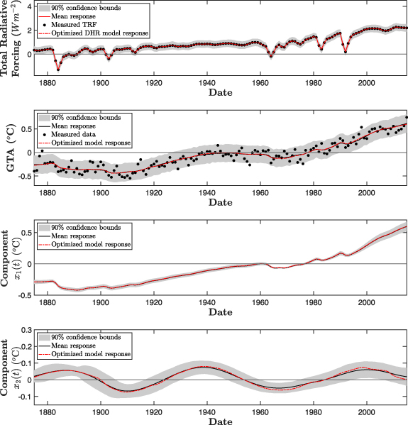
The MC analysis also enables us to generate random ensemble realizations of the model responses, from which the uncertainty in these responses can be evaluated as percentile bounds. The first panel in figure 6 shows the TRF with its associated 90 percentile bounds shown in grey, as estimated by the DHR model analysis. The second panel shows the mean response of the DBM model as a black line, once again with the 90 percentile bounds shown in grey, and the simulated response of the estimated model  shown as a red dash-dot line, which is virtually indistinguishable. The third and lower panels show the mean and 90 percentile bounds for the two components of
  , i.e.
  and
and  , respectively. These results, which are based on MC analysis using 5000 realizations, show that the model is statistically well defined and provides a reasonable explanation of the GTA record. The component state
  provides the dominant response to the TRF stimulus; while the second component state
  shows that the quasi-cyclic component is well defined but with wider uncertainty bounds that include the effects of some marginally unstable realizations.
Figure 6. Uncertainty in the TRF and the subsequent responses of x(t), x1(t) and x2(t) in the final DBM model, as obtained by MC analysis based on the estimated uncertainty in the model parameters.
Download figure:
Standard image High-resolution image
7. Conclusions
A third order differential equation model that accounts for both dynamic and stochastic responses can be identified objectively from the globally average climate data, without any pre-conceptions about the model structure or parameter values. Following the DBM modelling approach, however, the identified model can be interpreted in climatic terms. The associated re-evaluation of the ECS value and its range of uncertainty results in a useful improvement in the accuracy of resolving ECS when compared to current methods used in the IPCC context, with an ECS estimate of 2.29 ∘C with a 5%–95% confidence range of 2.11–2.49; and a TCR of 1.56 ∘C with a 5%–95% range of 1.43 ∘C–1.68 ∘C. When a high level of uncertainty in the forcing series is taken into account, however, the confidence range increases to 1.43 ∘C–3.14 ∘C for ECS and 0.99 ∘C–2.16 ∘C for TCR.
The model shows the globally averaged atmosphere as a parallel connection of two pathways. The upper pathway describes the dominant first order relationship between the TRF input and its more direct effect on the GTA, dominated by the effect of the anthropogenic increases of CO2. The second pathway is the less direct pathway, where, after the time delay of τ = 17.5 years, the TRF enters the negative feedback system with an integrator in the feedback path that, we suggest, represents possible heat exchange with the ocean, leading to a stochastic oscillatory mode of dynamic behaviour. This model explains the changes in the GTA very well and yields estimates and 5%–95% confidence ranges for the ECS and TCR and other climatic parameters, as well as the Natural Period (Pn ) of the oscillatory component.
The oscillatory component appears to explain the 'climate shifts' discussed, for example, by Swanson and Tsonis [39] and Essex and Tsonis [40]. It has an estimated period of 55.3 years, with a 5%–95% confidence range between 51.6 and 60 years. Most significantly in physical terms, the recession periods of this oscillation coincide with, and are used by the model to explain, the climate shifts ('pauses' or 'leveling') in the generally upward trend of the GTA. Moreover, the period of this oscillatory component is not that different from the 62.5 year period of the AMO, to which it can be related dynamically [25].
The linear model response assessed here is stimulated by the TRF input, which is dependent on carbon emissions and natural effects, such as volcanic activity. The possibility of nonlinearity was investigated but this did not reveal any significant evidence of nonlinear dynamic behaviour. It seems likely, however, that the linear-like behaviour is representing the relatively small perturbations of the climate over the 160-year observational interval and that the underlying system is almost certainly nonlinear. The lightly damped and regular behaviour of the DBM model's oscillatory component x2(t) could alter its character in the future depending on whether the stochastic effects become more prominent. Should this occur, more drastic changes could occur in future if this triggers nonlinear stochastic dynamic effects.
It is always important to evaluate how well defined and stable any estimated parameter is in statistical terms and a sequential estimation diagnostic check has shown that our re-evaluated ECS estimate of 2.29 ∘C is not only well-defined statistically but also has been close to a relatively stable level for the past 65 years. We can be reasonably confident, therefore, that it is statistically well-defined and useful, at least for short to medium time prediction and emission management purposes. Of course, the DBM model described in this paper has been inferred statistically from the data available when the present study was initiated and they can change over time. Also, like any model that has been inferred from a limited amount of normal operational data, without the ability to perform planned experiments, it provides a stimulus for future research. For example, we feel that further research is required on the possibility of heat exchange with the ocean using higher temporal resolution. This should help to establish how global teleconnection transport across ocean basins and processes (ENSO, PDO, NPI) might explain a possible GTA-AMO relationship.
The DBM approach used in this paper to model globally averaged climate behaviour provides a new, low dynamic order, stochastic model, together with new results that are intended to complement and extend the findings in recent papers and IPCC reports [3, 5, 32, 35]. It provides additional information that we hope will help to enhance the conclusions generated by more traditional climate models and methods of analysis.
Acknowledgments
The authors are very grateful to an anonymous reviewer whose valuable comments helped to improve the paper. JTB gratefully acknowledges the UK Research Councils funded Models2Decisions Grant (M2DPP035: EP/P0167741/1), ReCICLE (NE/M004120/1) and Newton Funded China Services Partnership (CSSP Grant: DN321519) which helped fund his involvement with this research. This work has benefited from engagement with and discussions in the Institute of Physics event 'Physics in the Spotlight', 2019.
Data availability statement
All the time-series data used in this analysis is freely available for research: http://cdiac.ornl.gov/trends/temp/jonescru/jones.html; www.pik-potsdam.de/∼mmalte/rcps/; www.cgd.ucar.edu/cas/catalog/climind/AMO.html. The models in this paper have been inferred statistically from the data record available when the present study was initiated and they can change over time. The data that support the findings of this study are available upon reasonable request from the authors.
Author contributions
PCY conceived and designed the study, as well as being responsible for all of the data-based mechanistic modelling analysis and the initial drafting of a larger paper and the associated technical report. PGA carried out the literature search and contributed the survey reported in section 2, as well as advising on other parts of the paper. JTB considered aspects of the ocean-atmosphere and long-term dynamic mechanisms that are relevant to the climate understanding. All three authors were responsible for adapting the paper into the required shorter format, as well as reading and approving the manuscript. The authors declare that they have no competing interests.