


Abstract
The carbon intensity (CI) of biofuel's well-to-pump life cycle is calculated by life cycle analysis (LCA) to account for the energy/material inputs of the feedstock production and fuel conversion stages and the associated greenhouse gas (GHG) emissions during these stages. The LCA is used by the California Air Resources Board's Low Carbon Fuel Standard (LCFS) program to calculate CI and monetary credits are issued based on the difference between a given fuel's CI and a reference fuel's CI. Through the Tier 2 certification program under which individual fuel production facilities can submit their own CIs with their facility input data, the LCFS has driven innovative technologies to biofuel conversion facilities, resulting in substantial reductions in GHG emissions as compared to the baseline gasoline or diesel. A similar approach can be taken to allow feedstock petition in the LCFS so that lower-CI feedstock can be rewarded. Here we examined the potential for various agronomic practices to improve the GHG profiles of corn ethanol by performing feedstock-level CI analysis for the Midwestern United States. Our system boundary covers GHG emissions from the cradle-to-farm-gate activities (i.e. farm input manufacturing and feedstock production), along with the potential impacts of soil organic carbon change during feedstock production. We conducted scenario-based CI analysis of ethanol, coupled with regionalized inventory data, for various farming practices to manage corn fields, and identified key parameters affecting cradle-to-farm-gate GHG emissions. The results demonstrate large spatial variations in CI of ethanol due to farm input use and land management practices. In particular, adopting conservation tillage, reducing nitrogen fertilizer use, and implementing cover crops has the potential to reduce GHG emissions per unit corn produced when compared to a baseline scenario of corn–soybean rotation. This work shows a large potential emission offset opportunity by allowing feedstock producers a path to Tier 2 petitions that reward low-CI feedstocks and further reduce biofuels' CI. The prevalence of significant acreage that has not been optimized for CI suggests that policy changes that incentivize optimization of this parameter could provide significant additionality over current trends in farm efficiency and adoption of conservation practice.
Export citation and abstract BibTeX RIS
1. Introduction
Since sustainable agriculture was described in the 1977 and 1990 'Farm Bills,' there has been a growing interest among the agricultural community in addressing the issue of 'sustainability' by developing and adopting integrated and innovative farming practices (National Research Council 2010, United States Department of Agriculture Office of the Chief Economist 2019). Several important farming practices, including conservation tillage, cover crops (CC), and nutrient management, have been shown to reduce greenhouse gas (GHG) emissions, or lower carbon intensity (CI), in crop production (ICF International 2016). Recently, these practices have received particular attention from the bioeconomy community and agencies for corn production, since corn accounted for 96% of all feed grain produced in the US in year 2018, and approximately 40% of the corn grain is purchased by biofuel producers who subsequently turn it into multiple products including ethanol, corn oil, and animal feed (United States Department of Agriculture Economic Research Service 2019). Accordingly, stakeholders have worked together to conduct thorough CI evaluation for various farming practices, adopting the life cycle analysis (LCA) approach to potentially reward low-CI feedstock production. The California Air Resources Board's Low Carbon Fuel Standard (LCFS) program adopted the LCA technique to calculate the CI of biofuels and issues credits to those that have lower CI than baseline gasoline or diesel.
In its current design, the LCFS allows for individual biorefineries to receive additional LCFS credits by lowering the CIs of their biofuels (Tier 2 pathway), creating a strong incentive for each biorefinery to minimize its GHG emissions by tying the plant's revenue directly to its carbon footprint. On the other hand, the LCFS program does not account for variations in upstream feedstock GHG emissions (i.e. farm input manufacturing and feedstock production), even though these activities contribute 36% to the well-to-wheels GHG emissions of corn-based bioethanol (Energy Systems. Argonne National Laboratory 2018) and show regional variations in energy consumption and fertilizer/chemical use (i.e. farming inventory) associated with diverse farming practices.
Several studies have addressed the regional variations in GHG emissions of feedstock production. For example, Pelton (2019) compiled county-level nitrogen (N) fertilizer share and application rate to quantify spatial GHG emissions from US county-level corn production. Smith et al (2017) documented county-level variability in yield, water consumption, and types of N fertilizers used, with the purpose of designing transparent supply chains. Neither study has considered the effects of land management and soil organic carbon (SOC) changes, which have been recognized as powerful carbon emission/sink sources in the agriculture sector (United States Environmental Protection Agency 2019).
To this end, Qin et al investigated the impacts of land management change (LMC) on the SOC stocks and the overall GHG emissions from corn-stover biofuel, by employing a process-based model to simulate spatially explicit (i.e. US county-level) SOC dynamics under various farming practices (Qin et al 2018). However, this study did not consider the variations in GHG emissions introduced by regionalized farming inventory. On the other hand, ICF International (2016) evaluated the potential of land management practices (LMC) to increase SOC stocks and dealt with regional variations in farming inputs. However, they utilized an empirical approach to estimate a national-average SOC sequestration value associated with tillage conversion under corn farming (West and Post 2002) and applied it to ten farm production regions in the US, while tillage practice can have different effects on SOC stocks in different regions because of local factors.
We aim to provide a complete quantification of CI throughout the cradle-to-farm-gate activities by conducting scenario-based analysis for selected farming practices, leveraging regionalized life cycle inventory data, and using spatially explicit SOC modeling tools. The impacts of these scenarios on the variations of feedstock GHG emissions are then evaluated in comparison with national estimates. Moreover, key GHG emission sources during the cradle-to-farm-gate activities for feedstock production have been identified. This information can enable feedstock producers to adopt regionally appropriate practices to minimize their emissions. Linking LCA information to farm-gate CI could allow Tier 2 certification of farms and provide strong incentives to adopt low-CI practices.
2. Materials and methods
2.1. Localized model and cradle-to-farm-gate GHG emissions
In this study, we applied the Greenhouse gases, Regulated Emissions, and Energy use in Technologies (GREET) model to conduct feedstock-level CI analysis (Energy Systems. Argonne National Laboratory 2018). GREET is widely used by regulatory agencies, industries, and research organizations to evaluate energy consumption, GHG emissions, criteria air pollutant emissions, and water consumption.
The system boundary of our analysis is limited to cradle-to-farm-gate activities, since we aim to quantify CI at the feedstock level. Three GHGs, namely CO2, CH4, and N2O, are considered (table 1), while direct soil CH4 emissions are excluded from our analysis since they are not significant (ICF International 2016, Locker et al 2019). The biogenic carbon uptake during the growth of corn grain is also excluded because it is assumed to be released back to the atmosphere during consumption (e.g. combustion of corn-based ethanol) (Canter et al 2016). The energy and material flows associated with upstream fertilizer/chemical manufacturing and feedstock production stages are the key components of cradle-to-farm-gate GHG emissions. Energy is consumed in planting, harvesting, and drying biomass. Fertilizers are used to boost the yield, while herbicides and pesticides are applied to reduce weed and insect damage. More details on fertilizer/chemical use data collection are available in the supporting information (SI) available online at stacks.iop.org/ERL/15/084014/mmedia.
Table 1. Key components of cradle-to-farm-gate GHG emissions and their associated data sources.
| Source | GHG | Data Source |
|---|---|---|
| Corn residue left in soils | N2O | 141.6 g N per bushel, |
| 1% (direct) + 0.225% (indirect) (Wang 2007) | ||
| Nitrogen fertilizer application | N2O | 1% (direct) + 0.325% (indirect) (Xu et al 2019) |
| Manure | N2O | 1% (direct) + 0.425% (indirect) (Wang et al 2012) |
| Urea fertilizer/lime | CO2 | CO2 emission due to urea and lime application to field (Energy Systems. Argonne National Laboratory 2018) |
| Soil carbon emissions | CO2 | Spatially explicit modeling using the parameterized CENTURY model (Kwon et al 2017, Qin et al 2018) |
| Input manufacturing | CO2, N2O, CH4 | United States Department of Agriculture (USDA) Agricultural Resource Management Survey (ARMS) (United States Department of Agriculture Economic Research Service 2010) and the GREET model (Energy Systems. Argonne National Laboratory 2018) |
| Energy consumption | CO2, N2O, CH4 | USDA ARMS (United States Department of Agriculture Economic Research Service 2010) and the GREET model (Energy Systems. Argonne National Laboratory 2018) |
In GREET, N2O emissions related to corn farming are calculated by the Intergovernmental Panel on Climate Change's (IPCC's) 2006 approach using emission factors (EFs) from various N sources (Dong et al 2006). Two sources of N inputs to soil are considered, namely, N from fertilizer application and N in crop residues left in the field after harvest. The content of N in crop residues is estimated using the harvest index and N contents of above- and below-ground biomass (Wang 2007). The N2O EFs are taken from the IPCC report (Dong et al 2006) or the literature review (Xu et al 2019).
GREET also considers the potential impact of SOC changes associated with farming practices in its GHG accounting. In the present study, spatially explicit SOC EFs were calculated using a process-based model (i.e. parameterized CENTURY model) that simulates SOC dynamics under various LMC. The parameterized CENTURY model was developed as an inverse modeling tool and it was calibrated for a long-term field trial in the US (Kwon and Hudson 2010) and North American croplands (Kwon et al 2017). Using the model, the SOC change rates are quantified for a 30 year time period in the 0–100 cm soil layer. One key assumption is that only current farmland can be adapted for different farming practices or LMC, while the non-farmland cannot, since the conversion of which to corn production would cause land use change-induced GHG emissions that have already been incorporated in biofuel LCAs (Qin et al 2018). More details on SOC modeling and associated data sources are provided in the SI.
Farm management scenarios have large effects on both upstream GHG emissions and LMC-induced SOC changes (Liu et al 2019b); therefore, outputs from GREET and SOC modeling were combined to provide a more comprehensive portfolio for assessing the GHG impacts of biofuels.
Note that all benefits and burdens associated with the implementation of scenarios are allocated to corn grain, since we treated corn stover as waste left in the field to reflect the current and near-future practice. The cradle-to-farm-gate GHG emissions, presented in the unit of CO2 equivalent (CO2e) per bushel of corn, were converted to the unit of CO2e per megajoule (MJ) corn ethanol by applying the corn-grain-to-ethanol conversion rate (0.35 bushels of corn per gallon of ethanol) and the lower heating value of ethanol (80.5 MJ per gallon) as the volume-to-energy unit conversion factor. We conducted this unit conversion since CI is commonly measured in the unit of CO2e per unit of energy.
2.2. Land management practices
We conducted analyses for a total of 192 scenarios with the baseline scenario depicting the business-as-usual (BAU) farming practice (table 2). SOC change is calculated as the relative change in SOC levels between a farm adopting alternative farming practice and BAU practice (Qin et al 2015). A negative SOC EF indicates net soil carbon gain, while a positive one indicates net SOC loss, compared to BAU. The national-average inventory for corn production was also estimated by applying corn acreage planted in each state as weighting factors and used as the comparison base.
Table 2. Baseline and alternative farming management scenarios considered.
| Management | Baseline scenario | Alternative scenario and environmental impacts | Key information | |
|---|---|---|---|---|
| Crop rotation with winter cover crops (CC) | Corn (year 1) -soybean (year 2) | Corn/rye - soybean | Increase residue carbon and nutrients in soils and reduce soil erosion | County-level yields; national-average energy use for CCs |
| Corn/rye - soybean/vetch | ||||
| Yield trend | Constant (a 10 year average from 2006 to 2015) | Increase (a historical trend from 1951 to 2015) | Increase residue carbon and nutrients in soils | County-level yields |
| Nitrogen fertilizer use | Constant rate | Reduced rate | Account for N credit of 45 kg ha-1 from vetch legume CC | County-level N application rate and type |
| Tillage type | National average | Three tillage types (conventional tillage, reduced tillage, no till) | Related to soil carbon sequestration and energy uses in tillage practices | State-level energy use for each tillage type |
| Manure application | No application | Application | Improve soil quality by adding organic carbon and nutrients | County-level manure application rate and type |
| New corn genetics (deep-rooting corn) | No adoption | Adoption | Improve productivity and/or input utilization efficiency of corn | Deep-rooting crop varieties |
| Enhanced-efficiency fertilizer (nitrification inhibitor) | No adoption | Adoption | Increases yield by 7% while reducing fertilizer N2O emission by 30% | |
2.2.1. Crop rotation with cover crops (CC)
The two-year rotation of corn and soybean adopted as BAU practice in this analysis results in higher corn and soybean yields compared to the respective monocultures (Behnke et al 2018). The county-level yield information for both crops was collected from USDA NASS (United States Department of Agriculture 2019) and utilized as inputs for SOC modeling with the assumption that their yields were recorded under the corn-soybean rotation. This assumption is justified by the prevalence of corn-soybean rotation in most of US Midwestern states, particularly those that produce large amounts of ethanol (Green et al 2018).
Winter CC planting in a corn-soybean rotation is gaining popularity as a conservation practice that improves SOC stock and provides agronomic and environmental benefits to subsequent cash crops (Marcillo and Miguez 2017). Winter rye (Secale cereale L.) and hairy vetch (Vicia villosa Roth) are considered in this analysis. The latter is a legume crop and can fix N from air into soil and provide an N benefit in the form of reduced N fertilizer requirement. The N benefit from a legume CC can be as high as 45 kg N/ha (United States Department of Agriculture Natural Resources Conservation Service 2014). Qin et al (2015) has implemented winter rye CC into the GREET by compiling the data on energy and material consumption due to winter rye cultivation and county-level rye yields (Feyereisen et al 2013). We collected the same type of information for hairy vetch CC (Undersander et al 1990, PennState Extension 2010).
2.2.2. Tillage
Tillage practices are classified by the percentage of residue remaining on the soil surface after planting. The rest of the residue is tilled back into the soil, since we assumed no stover harvest from the field. USDA reports the share of corn-planted area and the percentage of residue remaining for four tillage types, namely, conventional tillage (CT), reduced tillage (RT), mulch tillage (MT), and no tillage (NT).
To reduce the complexity of CI calculation and SOC modeling, we combined the RT and MT categories in the USDA classification into a single RT category (more details are available in the Tillage subsection of SI). Correspondingly, USDA's nation-averaged and state-averaged share of different tillage types can be applied in this analysis (table S5 in SI).
Compiling regionalized inventory on tillage share is necessary because different tillage practices incur different energy use rates. The diesel fuel requirements for various farming operations were obtained (University of Nebraska–Lincoln Institute of Agriculture and Natural Resources 2019) and the average diesel use rate was calculated for each tillage type (i.e. CT, RT, NT) (table S6 in SI). Note that the energy use rate for CT is almost 3.5 times as high as that for NT practice, providing the justification for incorporating this variation.
2.2.3. Enhanced-efficiency fertilizer (EEF)
N fertilizer management practices are crucial to improving crop yields and reducing N losses. While optimal rate, type, timing, and placement of N fertilizer are important factors, efforts have been made recently to develop stable EEF. It is reported that from 2005 to 2010, the use of EEF increased from 8.5% to 12.5% (Baranski et al 2018).
Here, we have evaluated one type of EEF—nitrification inhibitor that slows down the nitrification process where fertilizers are broken down to produce nitrates and N2O (ICF International 2016). According to a meta-analysis (Thapa et al 2016), nitrification inhibitor reduced N2O emissions compared to conventional N fertilizer by 30% and increased crop yields by 7%. These values are leveraged when compiling the regionalized inventory and modeling SOC change, by adjusting the crop yields and N2O EFs. Nevertheless, GHG emissions from the production and transportation of nitrification inhibitor are excluded from this analysis, since their contributions to the cradle-to-farm-gate emissions are minor (ICF International 2016).
2.2.4. Manure
Animal manure can be used as an organic fertilizer to improve soil quality by adding organic carbon and nutrients (e.g. N and phosphorus). County-level manure application rates and types were used for SOC modeling (Xia et al 2019). Manure application has already been implemented into the GREET model by compiling the data on energy consumption during manure transportation and application. The transportation distance for manure was estimated to be 0.367 mile and the transportation energy intensity was 10,416 Btu/ton manure/mile (Qin et al 2015). In term of application, it is assumed that 73.7% of the manure is applied via spreading and the rest is applied through direct injection (Energy Systems. Argonne National Laboratory 2018). Besides, the information on nutrient contents in different manure types is also collected.
Manure N has a higher N2O EF (1.425%) (De Klein et al 2006) as compared to fertilizer N (1.325%) (Xu et al 2019). The trade-off between SOC accumulation and N2O emissions for manure application is captured in our analysis. On the other hand, the nutrients in manure may reduce the inorganic N and phosphorus fertilizer input, but this possibility has not been considered.
2.2.5. New crop genetics
Improving productivity and/or input utilization efficiency of feedstocks is another important technology that has the potential to reduce the CI of biofuels. Recently, Paustian et al (2016) evaluated the potential of deep-rooting crop varieties to sequester SOC and reduce N2O flux; in this work, the CENTURY model was employed to estimate reference SOC stocks and simulate their changes associated with four hypothetically altered root growth scenarios. In the present study, we have incorporated the deep-rooting corn variety into the SOC modeling by adjusting root distributions, such that an additional 20% of corn root biomass in the 0–30 cm soil layer is moved to a deeper layer.
2.2.6. Yield trend
The yield of corn affects the yield of ethanol. If higher per-acre yield is achieved with the same level of per-acre chemical inputs, the CI of a MJ of ethanol produced from the field is lower. We analyzed two yield trend scenarios: constant and increasing yield. The constant-yield scenario assumes yield based on the 10 year average of county-level corn yield records from 2006 to 2015, while the increasing-yield scenario estimates yield using a simple regression equation derived from county-level corn yield records from 1951 to 2015 (table S7 in SI).
There are additional management practices available to improve the feedstock CI but are not considered in the present analysis. More descriptions are provided in SI.
3. Results and discussion
3.1. Changing farming practice impacts feedstock CI
3.1.1. Farming energy and material inputs
On the basis of national-average inventory data, feedstock production emits 28.5 g of CO2e per MJ of ethanol produced. Our results using regionalized inventory data compiled for the nine corn-farming states demonstrate a large degree of CI variation (figure 1). Compared to the baseline, Ohio has 12% higher GHG emissions while Minnesota has 13% lower. This is because an average Ohio corn grower uses more farm inputs and energy to produce a bushel of corn; while Minnesota farmers use less (table S2).
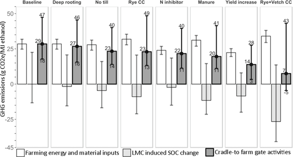
Figure 1. Impacts of farming practices on the following GHG emissions: (1) emissions related to farming energy and material inputs (including N2O emissions due to LMC); (2) CO2 emissions due to LMC-induced SOC change; and (3) overall cradle-to-farm-gate GHG emissions, calculated by combining the first two. To see the effect of each individual land management practice, one practice is varied at a time in the simulations. Each graph represents the specific practice that has been varied compared to the baseline scenario. To examine regional variation, the bar height reflects the national-average inventory, while the error bars represent the adoption of each practice at the state level.
Download figure:
Standard image High-resolution imageWhen compared to the baseline scenario, the yield increase scenario reduces the CI by 22%, as expected because the increase in yield means that fewer inputs are required for each bushel of corn. Similarly, CI reduction is observed when nitrification inhibitor is used, since its application is associated with a 7% yield increase and a 30% reduction in N2O emissions from N fertilizer (Thapa et al 2016).
If a vetch CC is planted after soybean in addition to the previous corn-rye year, more GHGs are emitted. This is because of the additional energy, fertilizers, and herbicides required for vetch cultivation, even after accounting for the N benefit from a legume CC. Similar trends are observed when comparing the scenarios where only rye CC is used and where manure is applied, since both scenarios require additional application of energy.
Finally, tillage intensity changes the cradle-to-farm-gate emissions. The NT practice consumes less energy and incurs less GHG emission compared to the average tillage practice. Since we assumed that changing to deep-rooting corn would not result in additional farming energy inputs, its GHG emissions remain the same as with the baseline scenario. It is important to reiterate that the discussion here (section 3.1.1) deals with farming energy and material inputs only. The net cradle-to-farm-gate GHG emission will be discussed separately in section 3.1.3.
3.1.2. LMC-induced SOC change
Using the parameterized CENTURY model (section 2.1), the effects of farming practices/technologies on SOC changes can be quantified. Figure 1 indicates that diverse land management practices can change the SOC stock. Practices and scenarios that lead to an increase in corn yield (i.e. yield increase scenario and nitrification inhibitor application scenario) contribute positively to SOC sequestration (i.e. negatively to SOC emissions). This finding is reasonable, since the SOC results are represented as relative changes compared to the baseline scenario, where corn yield is assumed to be constant.
The implementation of CC(s) contributes positively to SOC stocks. The corn/rye-soybean system can sequester, on average, 9 g of CO2 per MJ of ethanol produced. If a corn/rye-soybean/vetch rotation is used, an additional 17.6 g of CO2 can be sequestered, clearly showing the positive effect of CC on SOC preservation.
In terms of the tillage type, NT practice contributes positively to SOC preservation, since it disturbs the soil less, leading to a net CO2 sequestration of 4.6 g compared to the baseline value. The application of manure can also increase the SOC storage by 11.6 g per MJ of ethanol produced from corn harvested from that field. Deep-rooting corn adds more root biomass to soil, thus also helping to improve SOC content. On the basis of these results, the best practice for SOC conservation is no-till, deep-rooting, corn/rye-soybean/vetch rotation, with manure and nitrification inhibitor application, under a yield increase scenario.
Figure 2 shows large variations in the relative SOC sequestration achieved across Midwestern counties by shifting from baseline to best practice in terms of SOC conservation. The largest within-state variation was found in Nebraska, where the difference is 4453 kg CO2 per hectare per year. Even for the state that has the smallest within-state variation, i.e. Minnesota, the difference can still be as large as 2058 kg CO2 per hectare per year. By converting the units and distributing this impact to the resulting fuel, we calculate that changing practice results in a 43 g difference in CO2 emission per MJ of ethanol produced using the national-average corn yield of 166 bushels per acre. These results indicate the necessity of conducting localized assessment for SOC changes, since they are greatly impacted by local environmental parameters.
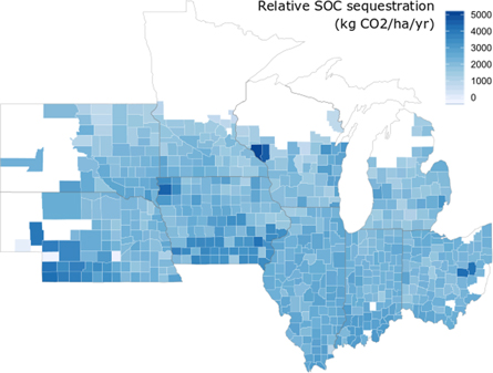
Figure 2. Spatially explicit modeling with parameterized CENTURY model for additional SOC sequestration achieved when shifting from baseline to best practice, at county-level resolution.
Download figure:
Standard image High-resolution imageWhile sophisticated process-based models are applicable to provide SOC quantification with less cost, the premise behind this assertion is that these models can be continuously calibrated and validated with databases of regional variations in management practices and their impacts on SOC changes for biofuel feedstock production. It should also be noted that SOC modeling results are simulated under certain assumptions (e.g. a 30 year-averaged climatic condition) and scenarios (e.g. constant yield versus increasing yield) related to model inputs, and thus should be interpreted with caution. Although longer simulation period or changing future climate may lead to different results, this 30 year simulation under current climate conditions provides sufficient justification for further evaluation through agronomic and policy experiments. Alternative climate scenarios require additional measurements and are beyond the scope of this simulation.
Alternatively, meta-analytic approaches similar to the IPCC Tier 1 methodology (De Klein et al 2006) can help to address the magnitude and uncertainty of SOC changes in agriculture to some degree (Paustian et al 2016). Eventually, field-measured SOC data may be used for CI certification.
3.1.3. Overall cradle-to-farm-gate GHG Emissions
The cradle-to-farm-gate GHG emissions are calculated by combining those from LMC-induced SOC change and those due to energy and material consumption. The combination of these two sets yields a comprehensive assessment of biofuel GHG emissions.
For the scenario involving both rye and vetch CC, the CI of feedstock production could be as low as 7.5 g CO2e/MJ, a 74% reduction compared to the baseline scenario. This finding again confirms that LMC has a large impact on the overall cradle-to-farm-gate GHG emissions.
Figure 1 also demonstrates the comparative magnitude of input-induced variation versus management-induced variation. By comparing the regional variations (i.e. the height of the error bar) to the national-average value for each scenario, we can infer that variations due to regionalized inputs and spatially explicit SOC modeling can be at least as great as the national-average values. This indicates the need for a land management practice database with high spatial resolution in order to support CI certification at the field level.
3.2. Identifying GHG emission hotspots and opportunities in feedstock CI
Figure 3 presents the highest-, average- (i.e. baseline), and lowest-emitting practices using national-average inventory from the 192 practices considered.

Figure 3. Highest-, average-, and lowest-emitting practices using national-average inputs (the black points indicate the net emission values). No regional variations are shown here, for the sake of showing differences among practices. The bars are segmented to show the contribution from each category of farming practice. The average emitting practice indicates the baseline scenario while the lowest emitting practice is no-till, deep-rooting, corn/rye-soybean/vetch rotation, with manure and nitrification inhibitor application, under a yield increase scenario.
Download figure:
Standard image High-resolution image
With the average-emitting practices, N2O emissions contribute 47% to the cradle-to-farm-gate GHG emissions. This is because of the high global-warming potential of N2O (265 g CO2e/g N2O) as compared to CO2. N2O emissions originate from fertilizer and biomass N inputs to soil. Therefore, reducing N fertilizer input while maintaining the yield is a highly effective way to reduce the cradle-to-farm-gate GHG emissions.
The results for the lowest-emission scenario show that increased SOC offers great opportunities for CI reductions. Further analyzing the results from the lowest-emitting practices reveals the trade-off between N2O loss and soil carbon accumulation. The lowest-emitting practices result in more N2O emissions, even after taking into account the N benefits from the vetch CC. This finding is mainly due to the return of additional CC biomass to the soil, which increases the amount of N input to the soil and leads to more N2O emissions. Under the model parameters used in this study, the added biomass contributes to SOC accumulation and leads to a net reduction in GHG emissions.
N fertilizer manufacturing accounts for 25% of the cradle-to-farm-gate GHG emissions, making it the second largest contributor. This fact suggests that it is important to track the amount and share of N fertilizers used. Planting a legume CC is a good option, since it offers N benefits, which reduces the GHG emissions due to N fertilizer manufacturing by 50%. New technologies that use renewable electricity to power ammonia synthesis or increase biological fixation through application of microbial amendments or N fixing traits in grain could dramatically cut or eliminate this portion of emissions.
Other main contributors include LMC-induced CO2 emissions and farming energy inputs; each contributes roughly 11% to the cradle-to-farm-gate GHG emissions. LMC-induced CO2 emissions have two components: CO2 emissions from urea application and CO2 emissions from lime application. Therefore, reducing the urea share in the N fertilizer mix and only applying lime when necessary could reduce these emissions. Regarding farming energy inputs, producers can reduce the tillage intensity to reduce the energy consumption. The last category considered is 'other chemical manufacturing,' which accounts for 7% of the cradle-to-farm-gate GHG emissions with the average-emitting practices.
When all emissions and SOC changes are combined as shown in figure 3, the lowest-emitting practices result in a net GHG sequestration of 15.9 g MJ−1, owing to substantial SOC sequestration.
Through an emission reduction program like the LCFS with CO2 priced at $160 per metric ton (California Air Resources Board 2019), valuable potential credits could be a strong incentive to encourage low-CI farming practices. Relative to the national-average cradle-to-farm-gate GHG emissions under the baseline scenario, a farmer implementing the lowest-emitting practices could be rewarded with $279/acre in the LCFS market. Further, regional variations that come from the regionalized farming energy and material inputs, and localized factors (i.e. soil and climate characteristics), may offer additional regionalized LCFS incentives.
4. Conclusions
Our analysis reveals remarkable differences in baseline values and suggests that farmers in the same region that use different practices may provide feedstocks with vastly different CI. Regulations such as the LCFS offer a platform to recognize these opportunities to encourage farming in more favorable regions and with lower-CI farming practices, to reduce the CI of biofuels in particular and agricultural GHG emissions in general. Furthermore, the regional variations and LMCs would have positive effects on other environmental attributes, providing co-benefits (Liu et al 2018a, Liu et al 2018b, Liu et al 2019a, Liu and Bakshi 2019, Rugani et al 2019). Some of the co-benefits that are particularly important to agricultural activities include soil fertility improvement, weed control, and nutrient runoff regulation. Thus, rewarding these practices under LCFS will achieve these co-benefits as well as CI reductions.
The goal of policy is to hasten trends and incentivize behavioral change. The additionality of a policy change refers to the ability of the policy to create additional change beyond a trend that already is occurring due to benefits outside of the policy. Because of the co-benefits to practice change, there may already be a trend toward broader adoption.
We feel that it is unlikely that a Tier 2 policy change would not create additional adoption of conservation practice. This is because none of these practices (no-till, etc) are new and these co-benefits are widely documented, which allowed us to perform this study. The fact that there is still significant acreage at higher CI than the local potential indicates significant additionality could be achieved with this incentive structure. To directly assess a new policy's effectiveness, regulators and researchers should monitor additionality through counterfactual analysis. The details of this research can be undertaken by future studies in estimating the economic impact of practice change, forecasting adoption of conservation practice based on current and past trends, and comparing geographic differences in biofuel markets.
This study is based on statistical data, approximation to finer regional resolution, and process model simulations to show CI reduction potentials of a future field-level certification system. Future systems capable of direct measurement of farm emissions will generate even more enticing options to incentivize outcomes rather than practice. Since all emissions are driven by local biological conditions in the soil and cropping systems, local monitoring can replace inventory-based systems and allow farmers to optimize their system for minimal emissions. The real-time, on-site monitoring system, e.g. chamber-based flux measurement (Maurer et al 2017), will offer insights on tradeoffs between yield, input applications, and agronomic practice leading to the generation of extremely low-CI practices, besides providing needed data for verification of Tier 2, field-level certification for LCFS and similar regulations.
Inclusion of biorefineries in Tier 2 CI systems has driven significant innovation at the plant level, including improved milling, drying, heat generation, yeast, co-product handling, and others. In much the same way, Tier 2 certification at the farm level will create incentives for the entire agriculture input sector to innovate around lower CI. This policy could drive broad innovation in agriculture including providers of genetically modified crops, input manufacturers, bio-engineers working on N-fixing organisms, data platforms, and precision agriculture sensors. Given the reach of the ethanol industry and the rapid adoption of valuable technology by farmers, new policies are expected to spur significant innovation and drive dramatic reductions in cradle-to-farm-gate GHG emissions.
Acknowledgments
This research was supported by the US Department of Energy Advanced Research Projects Agency-Energy under Contract No. 18/CJ000/01/01. The views and opinions of the authors expressed herein do not necessarily state or reflect those of the United States Government or any agency thereof. Neither the United States Government nor any agency thereof, nor any of their employees, makes any warranty, expressed or implied, or assumes any legal liability or responsibility for the accuracy, completeness, or usefulness of any information, apparatus, product, or process disclosed, or represents that its use would not infringe privately owned rights.
Data availability statements
Any data that support the findings of this study are included within the article.