Space-based quantification of per capita CO₂ emissions from cities

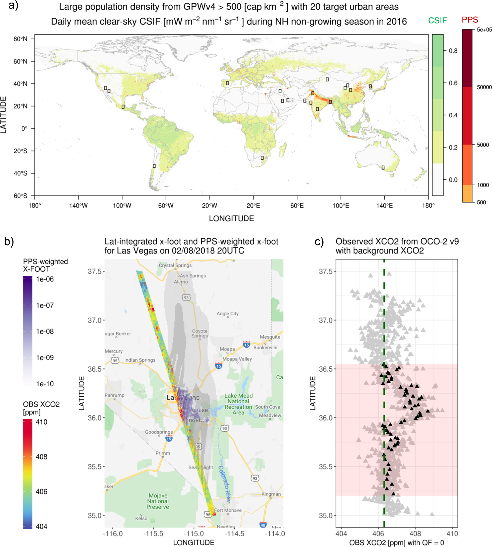
We select 20 cities across the midlatitudes over multiple continents (black boxes in figure 1(a)) based on favorable data quality and sampling patterns from OCO-2, minimal interference from vegetation, and relatively high population density according to the Gridded Population of the World (GPWv4; Center for International Earth Science Information Network CIESIN, Columbia University 2017). As an indicator of potential interference from vegetation, contiguous Solar-Induced Fluorescence (SIF) product (Zhang et al 2018) during north hemispheric non-growing season in 2016 is used to confirm minimal vegetation activities in target cities (figure 1(a)). We also examined the residual biogenic impact on our emission esimtates (SI appendix, Text D2 is available online at stacks.iop.org/ERL/15/035004/mmedia).

Zoom In Zoom Out Reset image size

Only satellite tracks whose upwind regions overlapping with the urban land during the non-growing season between September 2014 and April 2019 were analyzed for every city. The numbers of qualified satellite tracks span from 6 to 10 for northern hemispheric cities and are smaller for southern hemispheric cities (table S1). In the end, 134 satellite tracks were analyzed for emission estimates. For every track, we selected 50–90 screened satellite soundings with quality flags of zero from version 9 of OCO-2 lite files (OCO-2 Science Team/Michael Gunson, Annmarie Eldering 2018) to interpret track-specific urban XCO₂ signals (further explained in section 2.3). More details on the criteria for selecting cities and satellite tracks are described in SI appendix, text A.

To calculate CO₂ emissions from the observed urban XCO₂ signal and account for wind patterns affecting the satellite measurements, we adopted the atmospheric column version of the Stochastic Time-Inverted Lagrangian Transport (X-STILT, Wu et al 2018) model. 100 air parcels are released per vertical level in the atmospheric columns ('column receptors') corresponding to selected satellite soundings locate. To transport air parcels in the model, we used the Eta Data Assimilation System (EDAS) at 40 km grid spacing for the US cities and the global data assimilation system at 0.5° grid spacing (Rolph et al 2017) for the remaining cities. Errors in the wind fields and their impacts on per capita emissions are carefully investigated (section 2.4).

Next, source-receptor sensitivities, also referred to as 'footprints' (Lin et al 2003, Fasoli et al 2018), are generated at the horizontal resolution of 1 km × 1 km with a spatial coverage of 20°-lat × 20°-lon around each city center. 'Column footprints' (X_Foot, gray shading in figure 1(b)) are matrices that link potential upwind source regions to downwind atmospheric columns with units of ppm/(μmol m⁻² s⁻¹), with proper weighting using OCO-2 vertical weighting functions. Therefore, the upwind source regions of the satellite soundings are elucidated by X-STILT, which is also the region for examining the overlap with gridded population density maps (purple shading in figure 1(b)). Only population densities within source regions are taken into account to match with the corresponding urban signal observed by the satellite. Our objective approach of inferring source regions from the atmospheric model avoids having to impose, a priori, city boundaries.

The main dataset used to derive population density is the Gridded Population of the World (GPWv4, Center for International Earth Science Information Network CIESIN, Columbia University 2017). LandScan 2017 High Resolution Global Population Dataset (Dobson et al 2000) was used to evaluate possible bias in GPWv4 and its influence on scaling results (SI appendix, Text D1). Both products provide global population data at 1 km grid spacing. We adopted gridded GDP per capita (Kummu et al 2018), to assess how CO₂ emissions covary with socioeconomic variables.

We solve for an intensive quantity—the per capita CO₂ emissions (E_pc)—from all direct emitters over the source region affecting the satellite-observed XCO₂, as elucidated by X-STILT. Instead of attempting to calculate spatially explicit emissions, we treat the entire city as a whole and estimate an overall emission value per satellite track per city. The city-wide calculation is more robust against errors in the atmospheric model and their impact on emission estimates (Wu et al 2018).

E_pc per track per city is calculated as the ratio between an urban signal and a population density (PPS)-weighted column footprint as showed in equation (1):

$$\begin{eqnarray}&&\begin{array}{l}{{E}}_{{\rm{pc}}}=\displaystyle \frac{\displaystyle {\int }_{{l}_{1}}^{{l}_{2}}{\rm{X}}{\rm{C}}{{\rm{O}}}_{2.ff}\,(l)\,dl}{\displaystyle {\sum }_{x,y}\left\{{\rm{P}}{\rm{P}}{\rm{S}}(x,y)\displaystyle {\int }_{{l}_{1}}^{{l}_{2}}{X}_{{\rm{F}}{\rm{o}}{\rm{o}}{\rm{t}}}\,(x,\,y,\,l)\,dl\right\}\,}\\ \,\,\,=\,\displaystyle \frac{\langle {\rm{X}}{\rm{C}}{{\rm{O}}}_{2.ff}\rangle }{\langle XFP\rangle },\end{array}\end{eqnarray} \tag{ 1 }$$

where x, y are indices for the spatial grid, l is the latitude of every receptor/sounding. Spatial column footprints X_Foot (x, y, l) are generated at every 50–90 column receptors for a given track. The integral in the numerator is a latitudinally integrated XCO_2.ff enhancement due to fossil fuel combustion, or simply an urban XCO₂ signal. The entire summation in the denominator describes the overlapping region between X_Foot and PPS, which is revealed by the purple shading in figure 1(b).

More specifically, XCO_2.ff along the satellite swath are calculated as differences between a track-specific background and observed total XCO₂. We followed the forward-simulation approach presented in Wu et al (2018) to estimate an urban-enhanced latitude range (from l₁ to l₂; red ribbon in figure 1(c)) and background value over background region outside the latitude range. As not all source areas indicated by X_Foot are associated with high population density, gridded PPS from GPWv4 is convolved with latitudinally integrated X_Foot. Lastly, a linear regression curve is fitted whose slope serves as the one overall E_pc estimate per city (figure S1).

To examine the relationship between E_pc and PPS, a representative PPS value is required for every city. Instead of simply taking the average of PPS within a prescribed urban area, we calculate an effective population density (PPS_eff) as the footprint-normalized PPS:

$$\begin{eqnarray}&&\begin{array}{c}\begin{array}{l}{{\rm{PPS}}}_{{\rm{eff}}}=\displaystyle \frac{\displaystyle {\sum }_{x,y}\left\{{\rm{P}}{\rm{P}}{\rm{S}}\,(x,y)\displaystyle {\int }_{{l}_{1}}^{{l}_{2}}{X}_{{\rm{F}}{\rm{o}}{\rm{o}}{\rm{t}}}\,(x,y,\,l)\,dl\right\}}{\displaystyle {\sum }_{x,y}\displaystyle {\int }_{{l}_{1}}^{{l}_{2}}{X}_{{\rm{F}}{\rm{o}}{\rm{o}}{\rm{t}}}\,(x,y,\,l)\,dl\,}\\ \,\,\,\,\,\,=\displaystyle \frac{ \langle {XFP} \rangle }{ \langle X{F}_{{\rm{t}}{\rm{o}}{\rm{t}}} \rangle },\end{array}\end{array}\end{eqnarray} \tag{ 2 }$$

where XF_tot is the sum of footprints excluding those over lands or water bodies whose PPS are zero and X_Foot serves as a spatial weighting factor. In other words, population densities within the urban core are often weighted more, with more leverage on influencing the satellite-observed XCO₂. Therefore, PPS_eff vary among different satellite tracks under different meteorological conditions. Besides PPS_eff, we also calculated average PPS over the source region (PPS_upwind) to scale against E_pc as a sensitivity test (SI appendix, text D1). Similar to the calculation of PPS_eff, effective per capita GDP is also calculated for every track and city with spatial footprint serving as an areal weighting function.

The overall fractional error of E_pc is comprised of fractional errors in both observed urban signals and the atmospheric model (namely, from horizontal transport), according to E_pc calculation in equation (1). Vertical transport in X-STILT typically has a smaller uncertainty impact than horizontal transport (Wu et al 2018) and thus excluded from this study. Both observational and modeling errors are first quantified for each column receptor and then aggregated to track-level errors, after accounting for error covariances. Finally, by assuming statistical independence of errors between tracks, track-level errors decay as a function of $\sqrt{N},$ where N represents the numbers of tracks per city. Technical details of error quantifications are available in SI appendix, text C2.

The average urban signal observed by OCO-2 varies from 0.21 to 1.56 ppm (Lat-avg. column in table S1). Our estimates of E_pc range from 1.22 to 44.30 tCO₂ yr⁻¹. Estimates especially for low-emission cities fall within the same approximate range as national-level estimates from World Bank (World Bank 2014) or the Emissions Database for Global Atmospheric Research (EDGAR, Janssens-Maenhout et al 2019), even given differences in reporting years. Relative uncertainties of E_pc fluctuate from 16.0% to 46.9% for different cities (table S1). These uncertainties stem from a combination of measurement noise and errors in retrieving satellite XCO₂, background XCO₂, and the winds used to drive X-STILT.

A few cities stand out especially due to their high E_pc. Yinchuan is one of the four major coal production cities in China (Liu and Cai 2018). Due to rich coal resources and intensive coal production (Liu and Cai 2018), E_pc for Yinchuan is about five times higher than China's national-level estimates (table S1). In contrast, two other cities in China, Lanzhou and Xi'an, have comparable or slightly higher E_pc as the national average level. Middle Eastern cities are well-known for their natural gas and oil productions, while high E_pc of Johannesburg may be attributed to its coal-fired power plants as also seen from NO_x instruments like TROPOMI (Reuter et al 2019).

To further understand the unique emission structures for individual cities and plausible causes for the extremely high E_pc, we adopt sectoral breakdown of emissions from an emission inventory (EDGARv5.0, Crippa et al 2019, https://data.europa.eu/doi/10.2904/JRC_DATASET_EDGAR). These sectoral emissions, independent from OCO-2 based emissions, are utilized to calculate the XCO₂ percentage from every sector over all fossil fuel CO₂ (FFCO₂ sectors (ppm/ppm; in %). It is noteworthy that ∼12.9%–81.5% of the EDGAR-modeled XCO₂ enhancements are caused by power industries for different cities, and cities with high E_pc have high shares from their power industries (figure S2(a)). This finding underscores the importance of power plants in overall urban emissions (Singer et al 2014). As direct emissions from power industries are often unrelated to urban population (density) while emissions from buildings are expected to be related, we adopted the power-to-building XCO₂ enhancement ratio (figure S2(b)) as an indicator of the relative importance of power industries. This indicator identified Riyadh, Yinchuan, and Johannesburg as cities with heavy power industries given their high power-to-building concentration ratios.

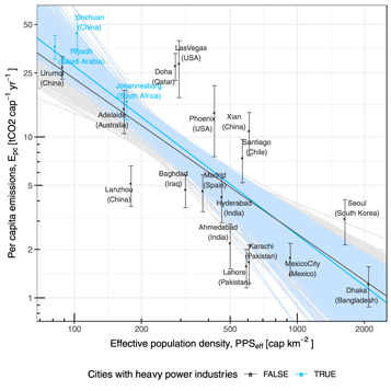
We next turn to the scaling relationship between E_pc and the effective population density (PPS_eff, equation (2))—an overall population density representing each city. E_pc generally declines as PPS_eff rises, even after uncertainties in E_pc are accounted for via Monte Carlo simulation. 5000 slopes of the E_pc–PPS_eff relation in logarithmic space from the Monte Carlo analysis (blue lines in figure 2) have a mean value of –1.06 with a standard deviation of 0.083. Since cities with heavy power industries (defined in section 3.1) may skew the E_pc–PPS_eff relation, we also report regression slopes with mean of –0.97 (gray lines in figure 2) after removing such cities from consideration.

Zoom In Zoom Out Reset image size

In addition to PPS, we examine the relationship between E_pc and per capita GDP (GDP_pc), which may shed light on E_pc's dependency on city-wide living standards. E_pc increases linearly with GDP_pc in logarithmic space, excluding a few industrial cities (figure S3). As a simple attempt to disentangle emission effects from GDP_pc, we carried out multiple regression fits using both PPS and GDP_pc in logarithmic space with E_pc's uncertainties accounted via Monte Carlo simulations. For all 20 cities, coefficients of GDP_pc are all positive with a mean of 0.59, while coefficients of PPS become less negative than the previous fit using just PPS as the explanatory variable (–1.06 to –0.83), implying that the decrease in E_pc is partially limited by the positive correlation between E_pc and GDP_pc.

Possibly to a lesser extent, E_pc–PPS relationship could be affected by other factors, e.g. emission seasonality caused by lack of summertime tracks, potential biases in GPWv4 and PPS_eff calculations, and minor residual vegetation influences gradient. For instance, E_pc using LandScan may differ from those using GPWv4, especially for Doha and Riyadh (5th versus 6th columns in table S1). However, sensitivity analyses suggest that the inverse E_pc–PPS relation is robust (SI appendix, text D). Lastly, population dynamics (e.g. transient versus resident population) may potentially affect the track-level E_pc and scaling slopes, but has not been studied in this paper due to unavailability of such datasets to our knowledge.

These are ultimately two different accounting methods for anthropogenic carbon emissions, also reflected in emission inventories that are either consumption-based (Davis and Caldeira 2010, Jones and Kammen 2014, Moran et al 2018) or direct emission-based (Oda et al 2018, Gurney et al 2009, Janssens-Maenhout et al 2019). Our estimates represent direct emissions from local emitters from a production-based perspective, in contrast to the concept of 'carbon footprint' or 'Scope 3 emission' (Moran et al 2018) which is calculated based on consumption (e.g. material, fuel, travel). Therefore, comparisons between estimates of direct emission and carbon footprint help identify various cities' roles as potential net carbon exporters/importers (Moran et al 2018). For example, Johannesburg, Riyadh, Urumqi, and Yinchuan have much larger direct emissions than carbon footprints, whereas Madrid and Seoul have smaller direct estimates (table S1), which likely implies the former three cities being net 'carbon exporters' and the latter two cities as 'importers'.

The scaling relationship obtained in this study is estimated based on a 'production-based/direct' emissions perspective, as informed from the satellite-observed CO₂ plumes that attribute emissions to sources at locations where the CO₂ is emitted to the atmosphere. However, urban residents rely on food and energy produced elsewhere. It is also possible that the scaling relationship could differ for the alternative consumption-based perspective, since residents of large and dense cities can consume goods and services that result in emissions elsewhere (Jones and Kammen 2014, Moran et al 2018). For example, it has been suggested that the carbon footprint per household (consumption perspective) and its variation with population density differs between urban cores, suburbs, and rural areas (Jones and Kammen 2014). However, we did not examine the population density dependence on CO₂ emissions at sub-urban scale or for subsets of population densities, given limited sample size and increasing complexity for calculating E_pc over suburbs and rural places from lower signal-to-noise ratio in XCO₂ and potential interference from biospheric fluxes.

While consumption-based emission accounting brings unique insights to international mitigation efforts, it may suffer from higher uncertainties due to emission reallocations (Peters 2008). Nonetheless, we stress that both the direct emissions perspective adopted in our analysis and the consumption-based emissions perspective are equally important and relevant, from both research and mitigation standpoints.