

Abstract
In view of the economic, social and ecological importance of Canada's forest ecosystems, there is a growing interest in studying the response of these ecosystems to climate change. Accurate knowledge regarding growth trajectories is needed for both policy makers and forest managers to ensure sustainability of the forest resource. However, results of previous analyses regarding the sign and magnitude of trends have often diverged. The main objective of this paper was to analyse the current state of scientific knowledge on growth and productivity trends in Canada's forests and provide some explanatory elements for contrasting observations. The three methods that are commonly used for assessments of tree growth and forest productivity (i.e. forest inventory data, tree-ring records, and satellite observations) have different underlying physiological assumptions and operate on different spatiotemporal scales, which complicates direct comparisons of trend values between studies. Within our systematic review of 44 peer-reviewed studies, half identified increasing trends for tree growth or forest productivity, while the other half showed negative trends. Biases and uncertainties associated with the three methods may explain some of the observed discrepancies. Given the complexity of interactions and feedbacks between ecosystem processes at different scales, researchers should consider the different approaches as complementary, rather than contradictory. Here, we propose the integration of these different approaches into a single framework that capitalizes on their respective advantages while limiting associated biases. Harmonization of sampling protocols and improvement of data processing and analyses would allow for more consistent trend estimations, thereby providing greater insight into climate-change related trends in forest growth and productivity. Similarly, a more open data-sharing culture should speed-up progress in this field of research.
Export citation and abstract BibTeX RIS

Original content from this work may be used under the terms of the Creative Commons Attribution 3.0 licence. Any further distribution of this work must maintain attribution to the author(s) and the title of the work, journal citation and DOI.
Introduction
Humans have modified their environment substantially, far beyond the natural variability in ecosystem processes (Zalasiewicz et al 2011), which has led to the proclamation of a new geological era, the Anthropocene (Crutzen 2002). A recent study located its onset at around the year 1950 (Waters et al 2016), after which a strong warming trend in climate was identified globally and particularly at high latitudes (IPCC 2013). In Canada, mean annual temperatures have risen on average by 1.7 °C since 1948, with the strongest increase along the West Coast (Environment Canada 2017). These rising temperatures coincide with an increase of almost 25% in atmospheric CO2 concentrations, emissions of which are attributable to human activities over the same period (IPCC 2013). Some concerns regarding climate change relate to its potential effects on ecosystems, including forests, that are of major importance for society. Forests cover nearly 40% of Canada's land surface and play a crucial role in the Canadian economy (Gillis et al 2005). Forest ecosystems also offer a large number of societally-relevant functions (Gauthier et al 2015), including the sequestration of a significant proportion of anthropogenic carbon emissions (Arneth et al 2010, Kurz et al 2013, Le Quéré et al 2018).
Concerns about the future of Canadian wood resources have led to a growing number of studies focusing on the assessment and monitoring of forest ecosystem characteristics. Major satellite observation programs began in the early 1980s and have provided information on the effects of environmental change and human activities on the geographical distribution of natural resources (Roy et al 2014). Such data allow mapping and monitoring the Earth's surface as a whole, with minimal budgetary considerations and time constraints that would limit spatial field observation campaigns to disparate networks of inventory plots in areas that are easily accessed (Zhang et al 2003, Sulla-Menashe et al 2016). The quality, accuracy and availability of remotely sensed data has been improving constantly over the last few decades. Moreover, a substantial proportion of these data is now available free of charge (Czerwinski et al 2014).
In contrast to remote sensing observations, a more field-based monitoring approach is the network of sample plots that has been established by federal and provincial authorities in Canada through national and provincial forest inventories (Béland et al 1992, Gillis et al 2005). These plots allow for the estimation of stand biomass through allometric equations that are based upon measurements of tree dimensions and the number of stems per hectare (Lambert et al 2005). Plot remeasurement provides information on temporal variation in stand productivity and permits the estimation of future (potential) productivity (Ciais et al 2008), an important management tool for adapting silvicultural practices to changing environmental conditions (Gillis 2011). A second field-based approach for studying growth trends relies upon dendrochronology, i.e., the measurement and dating of annual growth rings that allow linking spatiotemporal fluctuations in environmental factors to changes in tree growth rates (e.g., Berner et al 2011, Dietrich et al 2016, Babst et al 2018).
Many studies have focused on quantifying growth and productivity trends in Canadian forests using either one or multiple of these data sources, but reporting very different results. Rising temperatures combined with higher atmospheric CO2 concentrations have been assumed to improve forest productivity by lengthening the growing season (Eastman et al 2013) and increasing carbon assimilation rates (Long et al 2004). While several studies had indeed shown mainly positive trends for Canadian forests (Ju and Masek 2016, Hember et al 2017), other studies indicated a decreasing trend in growth and productivity rates (e.g., Chen et al 2016, Girardin et al 2016a). Heat stress that is caused by rising temperatures and an increase in the frequency and intensity of droughts, among other factors, have been suggested as explanations for these downward trends (Hogg et al 2005, Zhang et al 2008, Michaelian et al 2011, Girardin et al 2014). The lack of a clear tendency in growth and productivity estimates prevents policy makers from adequately defining annual allowable cuts, and foresters from determining appropriate silvicultural practices that maximize growth rates and forest yields.
Here, we provide an in-depth assessment of methodological aspects that could explain, in part, the contradictory findings of earlier studies. The first section of this paper focuses on the characteristics of the studied variables and spatiotemporal scales. We examine, whether the different methods target comparable eco-physiological processes, and to what extent observational scales and data resolution allow for robust comparisons. We then discuss biases associated with each method and how they may affect the calculation of growth and productivity trends. Finally, we propose the co-integration of the different methods as a means of improving estimates of growth and productivity trends across large forest biomes such as the Canadian forests. We conclude by pointing out the urgent need to adjust some of our established working methods to foster advances in this field of research. We also encourage intensified data sharing through open-access portals.
Methodology
Data sources and definitions
This paper is based upon a systematic review of trends in Canada's forest growth and productivity that were reported in peer-reviewed scientific articles. Articles were searched through the Google Scholar and ISI Web of Knowledge search engines using the following keywords: 'Canadian forest growth,' 'Canadian forest productivity,' 'Canadian forest inventory data,' 'Dendrochronological studies Canada,' 'Forest response to climate change,' 'normalized difference vegetation index (NDVI) trends Canada,' 'Productivity trends Canada,' 'Dendrochronology trends Canada,' 'Biases dendrochronology,' 'Biases forest inventory data,' 'Biases vegetation indices,' 'Uncertainties remote sensing data,' 'Uncertainties productivity calculation,' 'Uncertainties detrending.' Citations within the searched articles were also carefully checked and incorporated if they were relevant (backward search). While this work focuses on growth and productivity trends in Canadian forests, search results from other geographic areas have been retained for the purposes of discussion. In particular, these were studies that mentioned innovative methodological approaches that have rarely been applied in Canadian studies. The search did not include studies of productivity simulations that were derived from predictive models.
Throughout this systematic review, we shall refer to the terms 'growth' and 'productivity.' Here, we shall use the term 'growth' mainly to refer to secondary growth, i.e., the increase in tree diameter or basal area (e.g., Dietrich et al 2016, Girardin et al 2016a). Elsewhere, Assman (1970) defined 'forest productivity' as the increase in biomass or volume of wood per unit area and time. Researchers usually calculate this value as the difference in woody biomass between two measurement dates (e.g., Ma et al 2012, Hember et al 2017). In this paper, we shall use the term 'productivity' to refer to the change in living wood biomass that occurs within a stand or forested area between two measurement dates.
Different variables at different working scales
Interconnected but dissimilar physiological processes
We identified 44 studies that focus on the estimation of Canadian forest growth and productivity trends. Most of these studies rely upon remote sensing data, followed by forest inventory and tree-ring analyses (table 3, see specific examples in figure 1). Across all of these studies, Canadian forests experienced no significant change in growth, with a typical standardized growth rate of −0.52% per year with 95% bootstrapped confidence intervals [−2.27, +0.70] (average taken from n = 51 standardized growth rate samples, table 3). Half of the studies report positive trends, whereas the other half shows a decline in growth and productivity. Observed growth trends ranged from −24.5% yr−1 to +10% yr−1 (table 3). Some datasets show similarities, including NDVI from GIMMS 3g (Pinzon and Tucker 2014), aerial biomass inferred from provincial forest inventories, and trends in dendrochronological analyses of Canada's National Forest Inventory database (figure 1). During the late-20th century, the north-westernmost boreal zone showed negative trends, while the southeastern boreal zone displayed positive trends (figure 1). Despite this general tendency, one can see many differences in the signs and magnitudes of the trends within regions, depending upon the data source (table 3). Determining how much of these variable results are due to geography, versus methodological differences, versus random processes (errors) is a daunting task, and necessitates a closer look at the underlying eco-physiological and ecosystem processes that are captured by each of these methods.
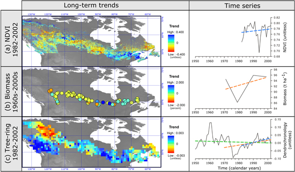
Figure 1. Left: comparison of spatially explicit trends across Canada's boreal forest assessed by (a) remote sensing (GIMMS 3g NDVI, data from Pinzon and Tucker 2014), (b) forest inventory (aboveground biomass, data from Ma et al 2012), and (c) dendrochronology (detrended basal area increments, data from Girardin et al 2016a). The periods covered by the trend analyses are indicated next to each map. Right: three examples of time series are shown for eastern Canada: (a) averaged NDVI over 50.875° N, 74.21° W, (b) aboveground biomass for 50.96° N, 74.01° W; (c) detrended basal area increments aggregated over 48.94° N, 74.76° W (see original papers for computation procedures). Also shown are linear regressions of values over time (a): 1982–2002 (blue dashed line), (b): 1971–1999 (orange dashed line), (c): 1950–2002 (green dashed line), 1970–2002 (orange dashed line) and 1982–2002 (blue dashed line).
Download figure:
Standard image High-resolution imageVegetation indices that are derived from remote sensing data are broadly used to approximate plant productivity (Berner et al 2011). The most commonly used vegetation indices are the NDVI derived from surface reflectance, and the leaf area index (LAI), estimated from other vegetation indices such as the NDVI on the basis of statistical relationships with field measurements. Vegetated areas typically exhibit NDVI values between 0.1 and 0.7 (Seth et al 1994, Wang et al 2005). Similar to spectral reflectance values (Carlson and Ripley 1997), vegetation indices are the expression of how much photosynthetic pigment is present in a given area (Nagai et al 2010, Piao et al 2014) and refer to 'greening' and 'browning' as seasonal trends in foliage area and pigment density. These indices are assumed to represent the state of the vegetation, its photosynthesis capacity (Myneni et al 1997b). In contrast, productivity estimates from forest inventories (typically quantified as aboveground biomass increment, ABI) correspond to stand-level biomass gains and losses between two inventory periods (Chen et al 2016, Hember et al 2017). These values inherently consider stand regeneration and mortality rates, as well as the stand-level increase in woody biomass of surviving trees (Hember et al 2017). Finally, tree-ring width (TRW), which is the most common parameter in dendrochronological studies, corresponds to the annual radial growth of a tree and represents the number and size of cells that are produced during the growing season (Berner et al 2011). TRW is often standardized (i.e., 'detrended') to obtain a dimensionless index (tree growth increment (TGI); ring-width index (RWI), a measure of the annual growth anomaly compared to the mean over a given time period (D'Arrigo et al 2004), although this step is increasingly being avoided when tree rings are used in an ecological context (Babst et al 2018).
Vegetation indices from remote sensing, aboveground biomass increments from forest inventories, and TGIs from dendrochronological studies are reported occasionally to be correlated with one another (Pouliot et al 2009, Girardin et al 2014, Vicente-Serrano et al 2016), but they represent the outcome of different physiological processes. While vegetation indices reflect photosynthetic capacity, growth-based metrics represent increases in woody biomass at different scales (stem: ring-widths or stand: ABI). These different proxies of growth and productivity refer to different processes of plant carbon uptake and use (leaf, stem, roots) and are correlated in a nonlinear fashion (Tateishi and Ebata 2004). RWIs refer mainly to the increase in radial diameter, i.e., secondary growth, and are thus not a direct measure of height growth or stand demographic processes, such as recruitment or mortality. Furthermore, the carbon that is sequestered in a given year will not only ensure the growth of that year, but can additionally sustain the tree's needs in the following years through the storage and remobilization of non-structural carbohydrates (Berner et al 2011, Richardson et al 2013). Consequently, a reduction in the tree's photosynthetic capacity or an increased carbon consumption for baseline metabolism during a drought year will reduce the carbon that is available for structural growth in the following year. This often leads to a 1 year lag between vegetation indices and radial growth increments (Berner et al 2011, Beck et al 2013, Seftigen et al 2018) and to significant autocorrelation in tree-ring time series (Zhang et al 2017). The correlation between remote sensing vegetation indices and tree- or plot-scaled proxies may also depend upon carbon sink strength of different organs (e.g., roots, shoot, needles or leaves) (Rieger et al 2017).
On the importance of working scales
Spatial scales
Spatial variability in growth and productivity trends is an important feature of Canadian forests (Girardin et al 2011, 2016a), and this variability occurs across latitudinal (Huang et al 2010) and longitudinal (Nishimura and Laroque 2011) gradients. Some authors also observed the importance of elevation (Parent and Verbyla 2010) and soil hydraulic regimes (Hember et al 2017), thereby emphasizing the role of spatially heterogeneous and temporally non-stationary factors that occur at different geographical scales (Anyomi et al 2014). Numerous interactions and feedbacks across time and space prevent analysts from defining clear boundaries between these scales (Miller et al 2004, Soranno et al 2014, Scholes 2017). As noted by Zhang et al (2003) and McMahon et al (2010), the different methods of assessing forest growth and productivity do not always operate at the same spatial scale.
Remote sensing often operates at regional scales where some local or stand-specific ecological and environmental processes are not captured as accurately as in field-based assessments (Goetz et al 2005, Beck and Goetz 2011, Piao et al 2014). Land cover maps allow grouping of the woody vegetation into large forest types (Zhou et al 2003), for which different productivity trends have been observed (Goetz et al 2005) that are potentially influenced by natural or anthropogenic disturbances (Boisvenue and Running 2006). Negative trends have been reported for areas that have been recently affected by a disturbance, whereas strongly positive trends are characteristic of forest regrowth responses (Hicke et al 2002a, Pouliot et al 2009, Beck and Goetz 2011, Ju and Masek 2016). Sulla-Menashe et al 2018 demonstrated that a large part of positive NDVI trends from remote sensing data could be associated with forest recovery after disturbance. Elimination of areas that were affected by a major disturbance could help improving comparisons between studies, as well as distinguishing the effects of climate change from those that are related to disturbances (e.g., Parent and Verbyla 2010, Beck and Goetz 2011, Sulla-Menashe et al 2016, Girardin et al 2016a, Hember et al 2017). However, algorithm-based identification of disturbed areas is error-prone and caution is warranted when interpreting these data (Sulla-Menashe et al 2016).
At the stand level, composition and demography can significantly affect forest productivity (Foster et al 2014). In addition to differences between individuals, some authors also have identified species-specific sensitivity to environmental stresses (Chen et al 2016, Wason et al 2017, Teets et al 2018). Such inter-specific differences are related to physiological thresholds and anatomical properties, such as root system morphology (Hember et al 2016), and would lead to different rates of biomass accumulation and growth trends (McMahon et al 2010, Girardin et al 2016a). Finally, at the finest scale of dendrochronological studies, growth trends of individual trees of the same species may differ even within the same stand (Buras et al 2016). This is likely due to demographic and genotypic differences between individuals or differences in microclimatic conditions, topography, soil properties and soil drainage (Wilmking et al 2005, Berner et al 2011, Brienen et al 2012, Girardin et al 2012, Girardin et al 2014).
Since ecological parameters that influence tree growth and forest productivity cannot be measured or controlled accurately, depending upon the spatial scale (figure 2), comparing trends from methods that operate at different scales is challenging. Therefore, it is risky to extrapolate results that were obtained at fine spatial scales to coarser scales (i.e., upscaling), and vice versa (i.e., downscaling) (Scholes 2017). For example, strong positive trends could be observed at the individual tree level, while the stand could experience lower or even negative trends resulting from a lack of regeneration or an increase in mortality rates (Hogg et al 2005, McMahon et al 2010, Groenendijk et al 2015). Similarly, an increase in vegetation cover could result in increasing values of vegetation indices over time, without a simultaneous improvement of tree growth rates (Mekonnen et al 2016). In this regard, one should proceed with caution when merging and interpreting results from several datasets based on different spatial scales.
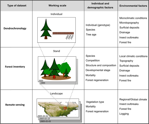
Figure 2. List of factors that could be measured or controlled at the different working scales (individual stem, sample plot/stand, landscape/global).
Download figure:
Standard image High-resolution imageTime scales
Growth and productivity trends are also temporally heterogeneous (Girardin et al 2016b, Hember et al 2017) (figure 1) and temporal scales differ between the three observation methods. First, remote sensing data have been available since the early 1980s (see table 1). The recording frequency varies from one week to one month for the most commonly used datasets (see table 1). Vegetation indices are usually rescaled to a monthly or annual step (e.g., Zhou et al 2001). In contrast, data from forest inventories have been available over the last 50 years on a 5- or 10-year time step (Hember et al 2017). Environmental conditions at the time of sampling are known; hence, each inventory campaign provides a snapshot of the sampled stands at a specific point in their life history (Biondi 2000, Bowman et al 2013). The temporal resolution of forest inventory data is coarse and does not allow visualizing inter-annual growth variations, e.g., following extreme climate events (Hember et al 2017). Finally, working with ring-width data allows analysts to assess inter-annual or seasonal growth variation of boreal species over the tree's lifespan (Berner et al 2011, Bowman et al 2013). However, tree rings in pre-instrumental times were formed in an unknown and uncontrolled environment (e.g., during the Little Ice Age, which ended in 1850), differing from current environmental conditions (Cook and Pederson 2011, Bowman et al 2013, Rieger et al 2017). Ring-width data, as well as remote sensing data, are available at a very fine timescale, which could also reduce the ability to detect subtle changes in growth due to a higher noise level (Verbesselt et al 2010).
Table 1. Spatial and temporal resolution and period covered by the most frequently used remote sensing datasets.
| Dataset | Spatial resolution | Period covered | Temporal resolution | Notes |
|---|---|---|---|---|
| AVHRR GIMMS | 1 km/8 km | 1978–now | Weekly/Bi-monthly | These products are derived from AVHRR data for which there are several sensor versions: 1 (1978), 2 (1981), 3 (1998) http://noaasis.noaa.gov/NOAASIS/ml/avhrr.html. Data correction methods differ between the three datasets. |
| AVHRR PAL | 8 km | 1981–2001 | 10 day/monthly | |
| AVHRR FASIR | 0.08°/0.25°/0.5°/1° | 1982–1999 | 10 day/monthly | |
| Terra-MODIS | 250 m/500 m/1 km | 2000–now | 16 day | https://terra.nasa.gov/about/terra-instruments/modis |
| GIMMS LAI3g | 0.08° | 1981–2004 | Bi-weekly | These products are derived from a merging of MODIS and AVHRR data http://modis.cn/globalLAI/GLOBMAP_LAI_DescriptionV1.pdf; http://glcf.umd.edu/data/lai/ |
| GLOBMAP LAI | 8 km, 0.08° | 1981–now | Bi-monthly (1981–2000), 8 day (2000–2015) | |
| GLASS LAI | 1 km, 0.05°/5 km | 1981–2012 | 8 day | |
| LandSat TM/ ETM+ | 30 m | 1982–now | 16 day | Landsat 4 (1982), 5 (1984), 7 (1999), Landsat 8 since 2013 https://lta.cr.usgs.gov/products_overview/ |
The direction and magnitude of trends may also depend on time-series length and their start and end dates (Lloyd and Bunn 2007, Hember et al 2017) (figure 1). Trends from half century-long series (e.g., 1950–2002; Girardin et al 2016a) that reflect a multi-decadal change in growth and productivity rates will not necessarily agree with those obtained from shorter time-series (e.g., 1984–2012; Ju and Masek 2016), which provide information on more recent changes. This would be particularly true in the context of a sudden reversal of trends, such as has been noted in some Canadian regions between the late 1980s and early 1990s (Wang et al 2011, Girardin et al 2014; see figure 1).
The spatiotemporal specificities of each observation method allow scientists to test for a large number of ecological assumptions. Forest ecologists rely on the very fine time resolution and wide geographical coverage of satellite data to observe continuous patterns of productivity trends across the landscape, and to formulate hypotheses about the potential link with other geographically-varying ecological phenomena, such as changes in the pattern of natural disturbances or in the phenology of woody species (Goetz et al 2007, Beck and Goetz 2011). Besides, the spatial unit of forest inventory data, i.e. the forest stand, makes them better suited to test more applied and forest industry-oriented hypotheses, for example regarding the best combination of stand structure and composition to maintain the highest yields under a warming climate (Millar et al 2007). Lastly, the individually-scaled ring-width data allow to quantify the between-tree heterogeneity in the growth response to environmental gradients occurring within a population (Buras et al 2016), and to link this heterogeneity with tree's growing conditions or morpho-physiological traits (Rozas and Olano 2013). However, despite their respective strengths, each of these three methods has its own weaknesses for assessing trends in tree growth and forest productivity.
Biases and uncertainties
Limitations of remote sensing data
Multiplicity of vegetation indices
The open availability of remote sensing data has led to a plethora of vegetation indices, each with its own calculation process. Because different vegetation indices are based upon different wavelengths, they do not convey the same information (Czerwinski et al 2014). Also, because of their remote nature, vegetation indices can be influenced by several environmental characteristics. For example, soil characteristics, such as soil colour, brightness and texture, or slope, are known to affect NDVI values (Raynolds et al 2013, Pattison et al 2015), especially in sparsely-vegetated (Czerwinski et al 2014) and mountainous terrain (Kerr and Ostrovsky 2003). Finally, NDVI is prone to saturation when focusing on highly productive areas (Pattison et al 2015), leading to less precise estimates of biomass changes in the most productive forests and possibly obscuring significant trends (Berner et al 2011). Since compiled NDVI time series are easily accessible (Ichii et al 2002), other existing and potentially more accurate indices are rarely used, such as the enhanced vegetation index (Baret and Guyot 1991, Czerwinski et al 2014, Jin et al 2016, Sulla-Menashe et al 2016, Karkauskaite et al 2017).
Spatial resolution
The limited spatial resolution of remote sensing time-series (table 1) may affect the trend accuracy of vegetation indices. The vegetation index value that can be attributed to a given pixel corresponds to the whole photosynthetic signal of the pixel (Olthof et al 2009, Berner et al 2011), and the detected trend will mostly be representative of foliage and productivity variation of the dominant species (Chen et al 2016), regardless of whether it is a tree species or not (Berner et al 2011). The influence of the type and amount of vegetation can be particularly problematic at high latitudes, where spurious positive trends that are observed in sparsely-forested areas (e.g., Guay et al 2014) could be due to an expansion of the understory vegetation (Berner et al 2011). Myneni et al (1997b) recommended that the type of vegetation cover be considered when using NDVI data. A lag between leaf expansion and photosynthetic capacity of broadleaved species is often proposed to explain the nonlinear relationship between vegetation index values and leaf area values of a given area (Nagai et al 2010). These resolution-dependent uncertainties may partly explain the largest proportion of positive trends for remote sensing-based studies compared to field observations (68% and 35%, respectively; figure 3(a)).

Figure 3. (a) Percentage of studies reporting positive (black) or negative (grey) growth and productivity trends for Canadian forests, by observational method (see table 1 for references). Pseudo-replication was considered as follows: in the case of two different studies published by the same author, the most recent study was selected; Chen and Luo (2015), Zhou et al (2001) and Ichii et al (2002) have been excluded. In the case of different results from the same study, with the same method and the same geographical area, but with different datasets, the sign of the average trend was considered (Zhu et al 2016). In the case of different results, with the same method, from the same study, but for different geographical areas, the trend corresponding to the widest geographical area (Chen et al 2014), or to the boreal forest (Goetz et al 2005, Bunn and Goetz 2006) was considered. In the case of two different results from the same study but with different methods, the two trends were retained (Berner et al 2011, Hember et al 2012, Bond-Lamberty et al 2014, Girardin et al 2014, Boisvenue et al 2016). Also shown is the number of studies taken into account by observational method and trend sign. (b) Percentage of studies according to their level of uncertainty, by observational method and trend sign. For information about the attribution of uncertainty levels, see the subsection 'Uncertainty assessment'.
Download figure:
Standard image High-resolution imageData quality
Data quality is crucial for detecting trends that result from subtle environmental changes, such as climatic gradients (Pouliot et al 2009, Guay et al 2014). Remote sensing data are prone to quality loss through environmental perturbations, mechanistic limitations, or sensor degradation (see figure 2 in Babst et al 2010). The main source of environmental perturbations are snow and cloud cover (Fensholt and Proud 2012). While the effect of snow cover can be avoided when focusing on snow-free seasons, cloud cover is a persistent concern, particularly for Landsat records of northeastern and western Canada (Roy et al 2008, Pouliot et al 2009). Cloud contamination induces artificially low NDVI values and could be responsible for the negative trends that have been observed for the Arctic region (Parent and Verbyla 2010). Existing algorithms that are used to remove cloudy pixels automatically (Sulla-Menashe et al 2016) are suboptimal (Slayback et al 2003). Removal of cloudy pixels also lowers the number of observations (Parent and Verbyla 2010, Fraser et al 2011, Ju and Masek 2016) and, thus, affects the capacity to detect significant trends (Pattison et al 2015). Uncertainties that are associated with sensor mechanics and post-recording corrections are related, among other things, to a lack of calibration, orbital drift, differences in viewing geometries, and to the use of different algorithms for atmospheric corrections (e.g., Roy et al 2008, Chen et al 2014). Because of these mechanistic limitations and error-prone correction algorithms, different data sources and sensors can provide differing NDVI values for the same geographical area (Sulla-Menashe et al 2016). This lack of robustness constrains the possibility of cross-studies comparisons (Fensholt et al 2009, Fensholt and Proud 2012, Raynolds et al 2013, Zhu et al 2016), as well as merging data from multiple sensors (Girardin et al 2016b), particularly for the Arctic region (Raynolds et al 2013).
Spatial heterogeneity and sampling biases
Effects of a non-random sampling strategy
Soil properties and vegetation types within ecological units are often heterogeneous (Lands Directorate 1986, Marshall et al 1999), and an incomplete representation of such heterogeneous conditions in analyses of Canadian forest trajectories may induce biases. Since field sampling is expensive and time-consuming (Vicente-Serrano et al 2016), forest inventory campaigns tend to target commercial species within intact, productive and mature forests (Hember et al 2012). Thus, the least productive (forested peat bogs or xeric forests) and the least accessible (mainly high-latitude areas) stands are underrepresented when considering these field-based observations (Boisvenue et al 2016). Dendrochronological studies, in contrast, often focus on the most climate-sensitive trees, i.e., individuals growing at the edges of their distribution range (Kaufmann et al 2004, D'Arrigo et al 2014, Charney et al 2016). This may explain the heterogeneity of trends from studies that are based upon plot inventories and dendrochronology (table 3, figure 3(a)).
Within a sample plot, the largest dominant/co-dominant and healthy trees are usually targeted for tree-ring or stem analyses (Duchesne and Ouimet 2008, Bowman et al 2013). This non-random selection of a subpopulation could bias the resulting growth trends. Sampling only the largest trees in recently regenerated stands, such as fast-growing trees, is referred to as 'big tree selection bias' in the scientific literature (Nehrbass-Ahles et al 2014, Groenendijk et al 2015, Brienen et al 2017). The resulting growth trends would be artificially high and unrepresentative of the entire population (Brienen et al 2012). In contrast, the selected living trees in the oldest stands could have experienced the slowest growth, especially for species with a short life expectancy, including most of boreal species. This selection of old, slow-growing individuals (Nehrbass-Ahles et al 2014) would lead to artificial negative growth trends (Brienen et al 2012). This is referred to as 'slow growth survivorship bias' or 'productivity survivorship bias' in the literature (Bowman et al 2013). Senescent trees would also artificially lower growth trends, which is referred to as 'pre-death slow growth bias' (Bowman et al 2013, Groenendijk et al 2015, Cailleret et al 2017). Also, trees that died prior to sampling are usually not accounted for when building chronologies (Swetnam et al 1999). This results in a loss of reliability and a biomass underestimation going back in time (Dye et al 2016), which is referred in the literature to as the 'fading record problem,' and could lead to apparent increasing growth rates.
Demographic biases, such as those discussed above, can lead to biased estimates of tree growth and forest productivity (Foster et al 2014) potentially exceeding by 150%–200% the average trend experienced by the whole population (Nehrbass-Ahles et al 2014). Therefore, there is a need to consider past demography when studying growth dynamics and variation in forest biomass (Hember et al 2016), especially through the sampling of deadwood and snags (Girardin et al 2011, Gennaretti et al 2014, Groenendijk et al 2015). A combination of dendrochronological data and simulated past biomass increments can permit accounting for growth rates of dead trees (Foster et al 2014). However, this approach does not account for abrupt and large mortality events, but instead relies upon the representativeness of the available dendrochronological data (Foster et al 2014).
Spatiotemporal fluctuation of inventory plot network
Analyses of repeated forest stand measurements have important advantages over other methods in that they enable the assessment of effects of stand dynamics, such as mortality and regeneration, together with competition for resources on productivity (Wilmking et al 2004, Foster et al 2014, Hember et al 2017). Since old stands exhibit lower productivity trends than mature and young stands (Girardin et al 2012, Chen et al 2016, Girardin et al 2016b), the use of the age of the oldest tree or time-since-disturbance as proxies for stand age are ecological parameters that are necessary for explaining productivity trends. Yet this variable can rarely be obtained because either the lifespan of trees is shorter than the typical stand-replacing disturbance return interval (and therefore, a minimum age is assigned to the stand), or age is estimated from core samples that are collected at breast height (1.3 m) or 1 m height, which can lead to an underestimation of tree age of up to 30% with shade-tolerant species (Marchand and DesRochers 2016). Other challenges include the effects of natural or anthropogenic disturbances that are superimposed upon ecological gradients (Girardin et al 2008) and stands that are, unfortunately, rarely resampled after disturbances (e.g. Hember et al 2012, Zhang et al 2015, Dietrich et al 2016, Hember et al 2017). A standard practice is the translocation or addition of new, non-disturbed stands to the initial inventory network (Hember et al 2012, Bowman et al 2013). Hence, post-disturbance recovery of productivity cannot be compiled. The resulting modification in the distribution of site quality, competition intensity, climatic conditions and age classes could induce further spurious negative productivity trends or mask positive trends (Bowman et al 2013, Hember et al 2017). To avoid uncertainties that are linked with these spatiotemporal fluctuations in the plot network, researchers need to consider only plots that were sampled from the first inventory campaign to the last one (Duchesne and Ouimet 2008, Ma et al 2012). This strategy leaves very few plots for analysis; for example, Ma et al (2012) retained less than 1% of the available plots in their study, in part, because of this criterion. Nevertheless, an important problem remains: random mass mortality events that are induced by natural disturbances are not considered (Körner 2003, Vanderwel et al 2013), which could result in underestimation of mortality rates and overestimation of the increase in aboveground biomass over time (Fisher et al 2008).
Uncertainties resulting from data processing
Spatiotemporal data aggregation
When working with large datasets, data rescaling, i.e., aggregation of data at a broader scale than the original scale, is a common practice that represents a trade-off between the amount of available information and its relevance to the study's purpose. Rescaling data at coarser spatial and temporal scales eases the interpretation and visualization of the results, but it also results in the loss of strong spatiotemporal variability in growth and productivity trends. Figure 4 illustrates how the direction of growth trends could vary when computed from chronologies successively aggregated at upper spatial scales. We utilized a subset of stem-analysis data from Quebec's Northern Ecoforest Inventory program, a network of 400 m2 sampling plots located in unmanaged forests (Létourneau et al 2008, Girardin et al 2012, Ols et al 2018). Individual ring-width series of black spruce (Picea mariana [Mill.] BSP) trees within Quebec's landscape unit 'Lac Robineau' (50.48–51.60N, 73.75–76.25W; n = 94 trees, up to n = 3 trees per plot were sampled) were detrended following Girardin et al (2016a) to obtain annually-resolved chronologies of growth coefficients. The detrended chronologies were then successively aggregated from the tree level to the plot level, ecological district and landscape unit by computing the median values per calendar year, and growth trends were computed over the period 1980–2005 as the regression coefficient between median chronologies and calendar years (as in Girardin et al 2016a). For illustration purposes, we highlight the very different results obtained from two distinct ecological districts regarding the direction of growth trends (figure 4). Sampling within the 'Coteaux du lac Wikui' ecological district suggested a decline in the growth of black spruce trees regardless of the working scale, consistent with the negative trend observed for the whole landscape unit. By contrast, sampling within the 'Coteaux du lac Montmort' ecological district revealed trends with reversed signs from one scale to another. Similarly, rescaling of vegetation indices when dealing with different spatiotemporal resolutions leads to an 'ecological fallacy' (Robinson 1950), i.e., making inferences about individuals based upon aggregate data and vice versa, and the broader 'ecological inference' problem (King 2013), viz., the difficulty of detecting significant trends (Slayback et al 2003, Fensholt et al 2009, Verbesselt et al 2010). Moreover, Chen and Cihlar (1996) and Chen et al (2014) highlighted differences in the way that vegetation indices are aggregated. Indeed, some authors consider either a maximum (e.g., Nagai et al 2010) or an average value (e.g., Chen et al 2014) at an annual or monthly timescale, or over the growing season of the trees (e.g., Slayback et al 2003). These differences would diminish the correlation between remote sensing indices and field data (Chen and Cihlar 1996), thereby leading to less reliable and less comparable trends.
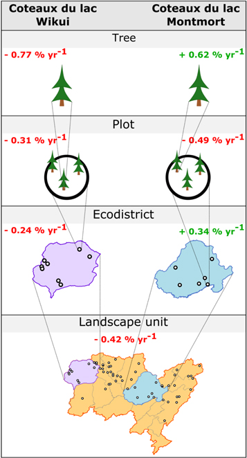
Figure 4. Illustration of some concerns resulting from data aggregation, using a subset of data from the Quebec's Northern Ecoforest Inventory program to infer black spruce 1980–2005 growth trends (in % of change per year) according to the working scale, from the individual tree to the landscape unit. Examples are provided for two different ecological districts within the landscape unit 'Lac Robineau' (50.48–51.60N, 73.75–76.25W).
Download figure:
Standard image High-resolution imageAllometric estimation
Allometric estimation is the extrapolation of some tree-or stand-level parameters that are difficult to measure directly (e.g., volume), based upon their strong statistical correlation with tree characteristics that are easily measured in the field, such as diameter at breast height. Thus, field measurements extending from local to national scales (Case and Hall 2008) are used to determine these relationships and to parameterize allometric equations, which are widely used to estimate stand productivity from forest inventory data (Lambert et al 2005, Wang 2006). Local equations are rarely developed because of the costs and logistics of field sampling. The number of field measurements remains low even for national equations. For example, the most widely used national equations that were devised by Lambert et al (2005) (e.g., Hogg et al 2008, Chen et al 2016) are based on relatively few field samples, with some provinces having very few measurements (see figure 2 in Lambert et al 2005). Even if one could assess the reliability of such parametric models via fit statistics, some concerns remain when extrapolating these models to broader scales without considering the whole set of ecological variables accounting for the variability in biomass within stands and regions. Since the heterogeneity of growing conditions increases with geographical extent, the use of a wide scale-parameterized equation (e.g., ecological region) also implies some uncertainties when results are to be analysed at a fine scale (Wayson et al 2015). Furthermore, biomass estimates from allometric equations rarely consider juvenile trees and belowground biomass, which leads to less accurate estimates (Keller et al 2001), particularly for slow-growing boreal stands (Bond-Lamberty et al 2002).
Estimate accuracy also relies upon the structure of allometric equations. Because of sampling issues, some variables that could improve estimation accuracy (Lambert et al 2005, Wang 2006), such as tree height, site quality index, ground-level stem diameter or stand age, are rarely considered (Bond-Lamberty et al 2002, Lambert et al 2005, Wang 2006, Case and Hall 2008). The use of well-documented tree-growth metrics from forest inventories could be a solution to the lack of field samples for parameterization. Despite these various sources of uncertainty, very few studies have tried to evaluate the accuracy of biomass estimates, because of the scarcity of field measurements (Wayson et al 2015). According to Bond-Lamberty et al (2002), the biomass of small or large trees would be underestimated, while the biomass of medium-sized trees would be overestimated when using allometric equations. Theoretically, when averaged over several trees of various sizes, these errors should cancel one another and lead to acceptable population-level values. In practice, since these errors are cumulative, biases from allometric equations could result in large uncertainties. Moreover, warmer weather conditions could alter allometric relationships as a result of modified carbon allocation strategies (Hasibeder et al 2015), leading to potential under- or over-estimations when inferring a future stand's aboveground biomass.
Detrending
Inter-annual variation in TRW is the result of multiple ecological and environmental processes. Detrending is a method of standardizing TRW data to remove unwanted (e.g., geometric) trends that can mask the desired environmental signal that is preserved in the measurements. As a standard procedure in dendrochronological analyses (Hember et al 2012, Sullivan et al 2016), detrending eliminates long-term growth trends that are induced, for example, by a tree's biology (tree size and local genotype; Savolainen et al 2007) and stand demography (age, competition). Numerous detrending methods have been developed over the years (Peters et al 2015), with the underlying aim of improving the retention of environmental signals. Depending upon the statistical procedure, several authors have observed differences in the magnitude and direction of growth trends that are derived from detrended series (Peters et al 2015, Sullivan et al 2016, Girardin et al 2016a). The most commonly used detrending method (i.e., fitting a curve through the time series) apparently eliminates part of the long-term signal and would be responsible for the lack of significant growth trends in many studies (Peters et al 2015). Regional curve standardization (RCS) and its derivatives (Helama et al 2016), which is seen as a potential solution to reduce detrending biases (Briffa and Melvin 2011), could induce artificially negative growth trends, according to Groenendijk et al (2015) and Brienen et al (2017). Sullivan et al (2016) observed a trend reversal when applying this method to chronologies that were averaged by size class. These negative biases are related to the trend detection step, which could partly explain the high percentage of dendrochronological studies reporting negative trends (70%, figure 3(a)), compared to remote sensing (31%) and forest inventory-based studies (60%). A recent detrending method that is based on mixed generalized additive models (GAMM), which was used by Fajardo and McIntire (2012), Camarero et al (2015) and Girardin et al (2016a), considered linear trends such as growth trends, together with nonlinear trends such as those linked with tree age and size (Peters et al 2015). GAMM could reduce detrending biases. Yet uncertainties remain about which part of the signal is exactly excluded or preserved from raw chronologies (Nehrbass-Ahles et al 2014), and which biases from collinear effects between variables could persist.
Uncertainty assessment
We have described above some of the most frequently reported biases, which could lead to erroneous conclusions about recent trends in tree growth and forest productivity. Therefore, one must deal with uncertainties that result from the inherent nature of remotely sensed data, from the sampling strategy, or from data processing prior to trend estimation. A quantification of these uncertainties could allow some confidence thresholds to be determined, thereby attributing some weight to the conclusion of the studies (Wayson et al 2015, Alexander et al 2018). According to Wayson et al (2015), uncertainties that are associated with allometric equations are responsible for up to 30% of the variability in productivity trends. This value and the qualitative information that is disseminated by other studies provide a preliminary assessment of the magnitude of uncertainties that are associated with the other sources of bias. We determined the uncertainty rates as follows.
First, remote sensing-specific biases are resolution-dependent. Uncertainties resulting from the use of coarse-grain datasets would be of similar magnitude to allometric estimations, and would decrease at finer resolutions. Thanks to correction algorithms, environmental or mechanistic noise would result in lower levels of uncertainty, especially when positive trends are detected (e.g., Sulla-Menashe et al 2016). The saturation phenomenon that is associated with NDVI datasets only weakens positive trends without changing their sign (Pattison et al 2015), but it would lead to a low level of uncertainty. Since most studies partly remove disturbed areas (e.g., Parent and Verbyla 2010, Beck and Goetz 2011), forest regrowth would only weakly affect productivity trends. In contrast, a non-random sampling strategy could lead to substantial uncertainty of magnitude similar to that imposed by allometric equations (Nehrbass-Ahles et al 2014, Alexander et al 2018). Furthermore, data processing for trend detection would affect growth trends, depending upon the method that is used. According to Sullivan et al (2016), the most commonly used detrending methods would lead to a higher level of uncertainty. In contrast, more recent methods, such as RCS and GAMM-based detrending, would be associated with lower levels of uncertainty (Peters et al 2015). Lastly, data rescaling should result in uncertainties of intermediate magnitude. A summary of the uncertainty rates that can be attributed to each source of bias is presented in table 2. One can see that uncertainty rates estimated here remained in the same order of magnitude whatever the observational method (tables 2 and 3). However, attribution of these different rates, although partly based on the literature review, remains highly subjective.
Table 2. A preliminary assessment of uncertainty rates attributed to different biases, depending on the sign of the observed trend. The aim of this table is to provide some idea of the magnitude for each uncertainty rate. See the subsection 'Uncertainty assessment' for information on the rate attribution.
| Bias | Data type | Uncertainty for positive trend | Uncertainty for negative trend | |
|---|---|---|---|---|
| Non-random selection of the stands, and temporal fluctuation of plot network | Forest inventory plots | 30% | 30% | |
| Non-random selection of the trees | Tree-ring | 30% | 30% | |
| Detrending | Conservative | Tree-ring | 20% | 30% |
| RCS/BAC/SCI | Tree-ring | 10% | 15% | |
| GAMM | Tree-ring | 5% | 5% | |
| Use of allometric equations | Forest inventory plots | 30% | 30% | |
| Resampling | 20% | 20% | ||
| Vegetation indices | Remote sensing | 10% | 10% | |
| Spatial resolution | 1–8 km | Remote sensing | 30% | 30% |
| 30–250 m | Remote sensing | 10% | 10% | |
| Atmospheric contamination of the satellite signal and calibration errors | Remote sensing | 5% | 15% | |
| Fire and insect outbreaks | Remote sensing | 10% | 10% | |
Table 3. Signs and values of growth and productivity trends from studies the areas of which include all or part of the Canadian territory (non-exhaustive list). (a) Trends that are based on a visual interpretation of the maps provided by the authors are indicated with an asterisk (*). (b) The determination of the last column ('Uncertainty') is explained in the subsection 'Uncertainty assessment'. The value reported here corresponds to the sum of all uncertainty rates assessed to the specified reference. NA for the growth trend ratio means that no quantitative value was available in the associated reference.
| Observational method | Trend sign (a) | Standardized rate (% per year) | Geographic area | Studied period | Dataset origin | Ecological process | Reference | Uncertainty (b) |
|---|---|---|---|---|---|---|---|---|
| Remote sensing | Negative * | NA | Northern Hemisphere | 1982–2008 | AVHRR GIMMS + MODIS | Productivity | Beck and Goetz (2011) | 45 |
| Remote sensing | Negative | −24.5 | Northwest Territories | 1982–2008 | AVHRR GIMMS | Productivity | Berner et al (2011) | 75 |
| Remote sensing | Negative * | −4 | World | 1981–2006 | AVHRR GIMMS 8 km | Productivity | de Jong et al 2011 | 65 |
| Remote sensing | Negative * | −1 | Northern Hemisphere | 1994–2002 | GIMMS 1° | Productivity | Angert et al (2005) | 65 |
| Remote sensing | Negative * | −1 | World | 1982–2009 | GIMMS | Productivity | Zhu et al (2016) | 85 |
| Remote sensing | Negative * | −1 | World | 1982–2009 | GLOBMAP | Productivity | Zhu et al (2016) | 85 |
| Remote sensing | Negative * | −0.45 | Northwestern America | 1982–2011 | AVHRR GIMMS 8 km | Productivity | Chen et al (2014) | 85 |
| Remote sensing | Negative * | −0.3 | Canada | 1981–2003 | AVHRR GIMMS | Productivity | Goetz et al (2005) | 85 |
| Remote sensing | Negative * | −0.3 | Northwestern America | 1982–2006 | AVHRR GIMMS 8 km | Productivity | Wang et al (2011) | 65 |
| Remote sensing | Negative | −0.2 | Quebec | 1981–2011 | AVHRR GIMMS3g 9 km | Productivity | Girardin et al (2014) | 75 |
| Remote sensing | Negative * | −0.06 | Northern Hemisphere | 1982–2003 | AVHRR GIMMS + MODIS | Productivity | Bunn and Goetz (2006) | 85 |
| Remote sensing | Positive * | 0.06 | Northern Hemisphere | 1982–2003 | AVHRR GIMMS + MODIS | Productivity | Bunn and Goetz (2006) | 75 |
| Remote sensing | Positive | 0.06 | Canada | 1984–2011 | Landsat TM L1T | Productivity | Sulla-Menashe et al 2018 | 35 |
| Remote sensing | Positive * | 0.2 | World | 1983–2005 | AVHRR GIMMS + MODIS | Productivity | Zhang et al (2008) | 95 |
| Remote sensing | Positive * | 0.3 | Canada | 1981–2003 | AVHRR GIMMS | Productivity | Goetz et al (2005) | 75 |
| Remote sensing | Positive * | 0.47 | Northwestern America | 1982–2011 | AVHRR GIMMS 8 km | Productivity | Chen et al (2014) | 75 |
| Remote sensing | Positive * | 0.56 | World | 1982–1999 | AVHRR GIMMS | Productivity | Zhou et al (2001) | 75 |
| Remote sensing | Positive * | 0.6 | World | 1984–2012 | Landsat + AVHRR GIMMS 8 km | Productivity | Ju and Masek (2016) | 35 |
| Remote sensing | Positive * | 0.75 | World | 1982–1999 | GIMMS + Pathfinder PAL | Productivity | Nemani et al (2003) | 85 |
| Remote sensing | Positive | 0.92 | Saskatchewan | 1984–2012 | Landsat | Productivity | Boisvenue et al (2016) | 45 |
| Remote sensing | Positive * | 0.94 | Northwestern America | 1982–1998 | AVHRR GIMMS | Productivity | Hicke et al (2002b) | 85 |
| Remote sensing | Positive | 0.97 | Northern Hemisphere | 1982–1999 | AVHRR GIMMS + FASIR 1° + Pathfinder 1° | Productivity | Slayback et al (2003) | 75 |
| Remote sensing | Positive * | 1 | Northern Hemisphere | 1982–1991 | GIMMS 1° | Productivity | Angert et al (2005) | 55 |
| Remote sensing | Positive * | 1 | Canada | 1985–2006 | AVHRR GIMMS 1 km | Productivity | Pouliot et al (2009) | 75 |
| Remote sensing | Positive | 1.25 | Yukon, northern Quebec | 1986–2006 | AVHRR 1 km + Landsat 30 m | Productivity | Olthof et al (2009) | 35 |
| Remote sensing | Positive * | 1.4 | World | 2000–2009 | MODIS | Productivity | Zhao and Running (2010) | 85 |
| Remote sensing | Positive * | 1.7 | Northern Hemisphere | 1981–1991 | AVHRR GIMMS + Pathfinder | Productivity | Myneni et al (1997a) | 75 |
| Remote sensing | Positive * | 2.4 | World | 1982–2009 | GLASS LAI | Productivity | Zhu et al (2016) | 75 |
| Remote sensing | Positive * | 2.5 | World | 1982–1990 | AVHRR Pathfinder | Productivity | Kawabata et al (2001) | 85 |
| Remote sensing | Positive | 3.75 | Alberta | 1982–2011 | AVHRR GIMMS | Productivity | Jiang et al (2016) | 75 |
| Remote sensing | Positive * | 8 | Northern Hemisphere | 1981–2000 | AVHRR GIMMS | Productivity | Piao et al (2006) | 75 |
| Remote sensing | Positive * | 10 | Northern Hemisphere | 1982–1999 | AVHRR GIMMS | Productivity | Zhou et al (2003) | 75 |
| Remote sensing | Positive | NA | World | 1982–1990 | Pathfinder AVHRR | Productivity | Ichii et al (2002) | 75 |
| Remote sensing | Positive * | NA | World | 1982–2000 | AVHRR Pathfinder | Productivity | Tateishi and Ebata (2004) | 55 |
| Forest inventory | Negative | −20.8 | Northwest Territories, Alberta, British Columbia, Saskatchewan, Manitoba, Ontario | 2000–2005 | Permanent sample plots | Productivity | Hogg et al (2008) | 60 |
| Forest inventory | Negative | −4.78 | Alberta, Saskatchewan | 1958–2011 | Permanent sample plots | Productivity | Chen and Luo (2015) | 60 |
| Forest inventory | Negative | −2.61 | Alberta, Saskatchewan, Manitoba, Ontario, Quebec | 1963–2008 | Permanent sample plots | Productivity | Ma et al (2012) | 60 |
| Forest inventory | Negative | −1 | Alberta, Saskatchewan | 1958–2011 | Permanent sample plots | Productivity | Chen et al (2016) | 60 |
| Forest inventory | Negative | −0.64 | British Columbia, Alberta, Saskatchewan, Manitoba | 1958–2009 | Permanent sample plots | Growth | Zhang et al (2015) | 30 |
| Forest inventory | Negative | −0.4 | Manitoba | 1999–2012 | Permanent sample plots | Productivity | Bond-Lamberty et al (2014) | 60 |
| Forest inventory | Negative | −0.38 | Ontario | 1950–1989 | NFBI | Productivity | Peng et al (2002) | 60 |
| Forest inventory | Positive | 0.35 | British Columbia | 1959–1998 | Permanent sample plots | Productivity | Hember et al (2012) | 60 |
| Forest inventory | Positive | 0.55 | British Columbia | 1959–1998 | Permanent sample plots | Growth | Hember et al (2012) | 30 |
| Forest inventory | Positive | 1 | Canada | 1961–2011 | Permanent sample plots | Productivity | Hember et al (2017) | 60 |
| Forest inventory | Positive | 1.2 | Saskatchewan | 1984–2012 | Permanent sample plots | Productivty | Boisvenue et al (2016) | 60 |
| Dendrochronology | Negative | −4 | Ontario | 1872–1999 | Wood cores | Growth | Dietrich et al (2016) | 75 |
| Dendrochronology | Negative | −2.2 | Northwest Territories | 1982–2008 | Wood cores | Growth | Berner et al (2011) | 60 |
| Dendrochronology | Negative * | −1 | Northern Hemisphere | 1951–2005 | Chronologies | Growth | Tei et al (2017) | 90 |
| Dendrochronology | Negative | −0.9 | Quebec | 1950–2005 | Permanent sample plots | Growth | Girardin et al (2012) | 90 |
| Dendrochronology | Negative | −0.1 | Canada | 1950–2002 | Permanent sample plots | Growth | Girardin et al (2016a) | 65 |
| Dendrochronology | Negative | −0.086 | Quebec | 1950–2007 | Permanent sample plots | Growth | Girardin et al (2014) | 90 |
| Dendrochronology | Positive | 0.55 | Saskatchewan, Manitoba | 1950–1994 | Wood cores | Growth | Brooks et al (1998) | 90 |
| Dendrochronology | Positive | 0.57 | Manitoba | 1912–2000 | Temporary sample plots | Growth | Girardin et al (2011) | 70 |
| Dendrochronology | Positive | 1.4 | Manitoba | 1999–2012 | Wood cores | Growth | Bond-Lamberty et al (2014) | 90 |
| Dendrochronology | Negative | NA | Northern Hemisphere | 1902–2002 | Chronologies | Growth | Lloyd and Bunn (2007) | 90 |
An overall uncertainty rate was computed for each of the referenced studies, as the sum of uncertainty rates (i.e., values in table 2) potentially affecting the results that were reported in the study (table 3, last column). For example, Dietrich et al (2016) suggested that results could be biased both by stand- and tree-level sampling biases (both 30% uncertainty rates), and by biases from RCS detrending (15% uncertainty rate for the detection of negative trends), which leads to the assignment of an overall 75% uncertainty rate. These uncertainty rates were finally segregated into four classes, i.e. four levels of uncertainty, as follows: a 'low' level of uncertainty was attributed to studies whose uncertainty rate is below 40%, a 'moderate' level of uncertainty to studies whose rate is comprised between 40% and less than 60%, a 'high' level of uncertainty to studies whose rate is comprised between 60% and less than 80%, and a 'very high' level of uncertainty in the case of studies whose rate is equal to or above 80%. Based on this classification, one can see that a substantial proportion of trends reported in the literature, whatever their direction or the observational method they originated from, is subject to a 'high' or 'very high' level of uncertainty (figure 3(b)). As a guideline for forest ecologists, the approach we proposed remains voluntarily illustrative and uncertainty rates will have to be improved before using them to correct previously assessed trends. Given that some biases may cancel out or amplify one another, further field-based quantification is needed.
Co-integration and a multidisciplinary approach
Make these approaches complementary, not contradictory
When studying growth and productivity trends of Canadian forests, one might think that the use of a given observational method would provide a more accurate assessment of recent trend directions than other methods. Yet the response of the forest ecosystem to global change depends upon multiple interactions and feedbacks that occur at different spatial and temporal scales (Pouliot et al 2009). A disturbance occurring at a given scale will have repercussions at the other scales. When studying the forest ecosystem as a whole, one should simultaneously consider all working scales, which involves the combination of all available methods, viz., dendrochronology, forest inventory data and remote sensing observations (Berner et al 2011, Girardin et al 2014, Boisvenue et al 2016, Girardin et al 2016a). Merging data from different approaches would allow for cross-validation (Nagai et al 2010, Bowman et al 2013, Czerwinski et al 2014), facilitating the determination of representative growth trajectories for the entire Canadian forest (Boisvenue et al 2016).
Co-integration of different observational methods
Different spatiotemporal coverages of the three observational methods that are discussed throughout this paper are currently complicating comparisons between studies. The comparison of the three different approaches would first benefit from the study of a common period of time. As discussed in the section Different variables at different working scales, different time windows (table 3), as well as a trend reversal from the early 1980s (Wang et al 2011, Girardin et al 2014; see also figure 1), reduce the possibility for cross-validation of the results. Historical growing conditions could affect current tree growth (Baral et al 2016), but recent growth rates would be more representative of current directions of Canadian forests. Thus, a recent time window, e.g., 1981 to the present, would be an appropriate choice when studying growth trajectories. In particular, only the last 30 years of growth are to be considered when estimating growth trends from ring-width series of centuries-old trees because of the potentially compensation effect of older tree-rings leading to trend estimates that are not reflective of recently occurring changes in growth rates.
Second, studies focusing specifically on the post-disturbance recovery of productivity through the measurement of seedlings and saplings are scarce (Van Bogaert et al 2015). To improve our knowledge regarding current and future growth directions, data that are available on the growth of young trees from studies comparing different developmental stages (e.g. Chen et al 2016) or comparisons of height growth rates of trees based upon time-since-disturbance (e.g., Fantin and Morin 2002, Gamache and Payette 2004, Andalo et al 2005, Leroy et al 2016, Marchand and DesRochers 2016) must be merged into a meta-analysis. Given that no transformation is applied (raw data), sampling height values from stem-analysis data that are taken from permanent sample plots are free from the uncertainties that are associated with dendrochronological data or with allometric estimates. A few sources of bias could originate from approximations of heights of sampling when cutting the radial sections. Thus, the time interval that is necessary to reach a given height can be extracted and used as a proxy for recent changes in primary growth rates, thereby complementing the information on radial growth that is provided by RWIs. As an applied case study, figure 5 provides an example of cross-validation between two data sources. Figure 5(a) displays height-growth curves from stem-analysis data of 1878 black spruce trees from Quebec's Northern Ecoforest Inventory program (Létourneau et al 2008). In figure 5(b), the time that was required for a black spruce tree to grow from 1 to 12 m was superimposed upon detrended mean annual basal area increments (BAIs) that were based on 200 plot-level chronologies (data from Girardin et al 2014). The time to grow from 1 to 12 m was computed as the difference between the age at which the tree reached the sampling height (calendar year attributed to the stem-section's ring of cambial age 1, minus calendar year attributed to the oldest tree-ring of the tree) and the age when reaching a height of 1 m. The two different approaches displayed a similar pattern of growth declines throughout the 20th century.

Figure 5. Cross-validation of forest growth trajectories using a combination of two different approaches. (a) Height-growth curves for Picea mariana trees north of the limit of commercial forests. (b) Time for a black spruce tree to grow from 1 to 12 m in height, superimposed on regional black spruce tree growth index (TGI, a unitless value computed as the average of detrended tree-ring width measurements) chronology, (data from Girardin et al 2014).
Download figure:
Standard image High-resolution image
Given their broad geographical extent, remote sensing data must be used first to assess the geographical variation of productivity trends of forest ecosystems, as a general overview. Since suboptimal targeting of forested areas can bias productivity trends, the use of maps that include not only forest cover, but also site characteristics (rather than land use or land cover maps) is advised to locate forested stands accurately and to exclude non-forested regions. These maps can facilitate the linking of remote sensing-based trends with ecological parameters, for example, to differentiate trends between stands of different ages or compositions. For an even more accurate comparison with inventory- and tree-ring-based studies, one must target only pixels including field-sampled areas (e.g., Berner et al 2011, Girardin et al 2014). In a second step, forest inventory data must be used to target stands of interest, for example, to study the specific response of stands to climate change according to their age or density. Last, dendrochronological and height-growth data can be used to cross-validate trends at stand- and individual-levels, and to specify whether the observed trends are due to changes in stand demography (i.e., mortality rate or recruitment efficiency) or to modifications of individual growth rates.
Need for improvements
To improve comparisons between studies relying on forest inventory data and to increase the quantity of potentially usable data for meta-analyses, standardization of sampling protocols appears necessary (Peters et al 2015, Chen et al 2016). This is the particular goal of establishing Canada's National Forest Inventory program, which is a systematic or random sampling strategy that is applied across Canada's forests. Measurement of as many environmental variables as possible that are undertaken through this inventory will help determine potential drivers of growth trajectories.
Open datasets through public repositories (e.g. DRYAD7 , PANGEA8 ) have the potential to accelerate advances in environmental sciences (Wolkovich et al 2012), especially in the field of forest ecology where large datasets are highly valuable for global-scale studies (Soranno et al 2014). The collaborative effort that was initiated by the International Tree-Ring Data Bank9 (NOAA, Boulder, CO, USA) to centralize and make available all data from dendrochronological studies (Grissino-Mayer and Fritts 1997) should be strengthened with data that have been collected from national and provincial forest inventories, together with unpublished data contributed by research laboratories (Babst et al 2017). Some authors highlight the lack of a systematic assessment of data quality (Goetz et al 2005, Gleckler et al 2008, Ju and Masek 2016), which is necessary to quantify trend accuracy. To this end, it would be a wise systematic strategy to include detailed metadata when sharing datasets, especially information regarding sampling methods and known biases (Daly 2006). Open data and metadata will also facilitate the attribution of a rate of uncertainty to the computed trends, notably through the dissemination of the size of the sampled population (e.g. number of pixels effectively accounted for, size of the area for which a positive versus a negative trend was observed) of remote sensing-based studies. Because of improved knowledge about what is already available and what is still lacking, data sharing could also stimulate data collection worldwide (Wolkovich et al 2012). Making data sharing a standard requirement for scientific publication (Whitlock et al 2016) could thus help filling the gap between studies whose primary aim is to assess forest growth and productivity from direct observations and studies more specific to other research fields, such as ecophysiology or genetics.
The trend detection step is an important source of uncertainty in dendrochronological studies. Most currently used detrending methods were developed with a view to reconstructing past climatic conditions from inter-annual to multi-centennial variations in growth rates; they are not necessarily appropriate to quantify and assess long-term growth trends. More flexible statistical methods that are capable of retaining both long- and short-term growth trends would allow analysts to adapt detrending procedures to these emerging objectives. Because trees respond individually to environmental gradients, the trend detection step should be performed at the individual scale. The challenge for unbiased detrending is to accurately distinguish and remove the proportion of long-term trend that is induced only by the tree's biology (age and size), and to retain the signal that originates from both environment and climate. Currently, the GAMM-based approach seems the most appropriate method because it allows for some control over what trend is being removed from the raw chronology, given the possibility for including some environmental variables. An approach that permits the determination of an average biologically-induced growth trend at the individual scale, such as the C-method that was developed by Biondi and Qeadan (2008) for shade-intolerant species, also seems promising. Some work should be done to adapt this method (i.e., the underlying mathematical equations) for slow-growing boreal species. Dendroecologists are increasingly attempting to move away from detrending, for example, by using BAI instead of TRW or by combining TRW data with inventories (Evans et al 2017). Pending these improvements, the suggestion of Peters et al (2015) and Girardin et al (2016a) to test and compare different detrending methods for cross-validating the resulting growth trends is meaningful. This comparison should be supplemented by an assessment of the effects of coring or harvesting height on the accuracy of the detrending step (Autin et al 2015).
Conclusions
Throughout this systematic review, we have highlighted several elements that contribute to the divergences observed in growth and productivity trends of Canadian forests. By the different working scales and physiological processes considered, observational methods utilized when assessing forest trajectories are suitable to test a broad range of ecological hypotheses, both from an applied and a more theoretical standpoint. Concurrently, these differences prevent an accurate comparison between studies. Trend calculation is also affected by several biases that are inherent to these methods, which further contributes to the observed variation in growth and productivity trends. Because the biases for over- and underestimation are comparable across these methods (table 2), we cannot attribute contrasting results from growth or productivity trend estimates simply to these scale and methodological concerns. The inability either to control or to measure some ecological or disturbance-related processes when working at a broad geographical scale is an additional difficulty that impedes the comparison, cross-validation, and joint use of datasets from multiple observational methods.
Several improvements would help clarify the current and future trajectories of forest communities. We argue that we must work towards generalizing growth trends that are inferred from dendrochronological studies and productivity trends from forest inventories. In proceeding in this manner, one must be careful about sampling biases and the degree to which plot networks are representative of the focal area. Better sampling strategies (Nehrbass-Ahles et al 2014, Babst et al 2017), together with integration of remote sensing (e.g. Jucker et al 2017) or forest inventory data (Evans et al 2017), could help. A co-integration approach is a means of emphasizing the respective advantages of each method, while limiting their respective disadvantages. The study of a recent and common period of time, a better targeting of the data, a focus on recently regenerated stands, and a hierarchical use of different types of data would provide a better idea of changes that have recently occurred in growth and productivity rates of forest ecosystems. Finally, harmonized sampling protocols, together with a revision of some empirical, but out-dated data processing procedures and a generalization of open datasets would improve the accuracy of the resulting trends.
Acknowledgments
This research was conducted as part of the International Research Group on Cold Forests. This study was made possible thanks to the financial support provided by the Strategic and Discovery programs of NSERC (Natural Sciences and Engineering Research Council of Canada). Additional financial support was provided by the Canadian Forest Service and the UQAM Foundation (De Sève Foundation fellowship and TEMBEC forest ecology fellowship). FB acknowledges funding from the EU-Horizon2020 project 'BACI' (grant 640176). We thank Philippe Juneau, Émeline Chaste, Benjamin Andrieux, Mathilde Pau, Marine Pacé, Claire Depardieu for proofreading a previous version of the manuscript and three anonymous reviewers for their constructive feedbacks. We also thank Isabelle Lamarre and W F J Parsons for English language editing.