

Abstract
Forest structure—the height, cover, vertical complexity, and spatial patterns of trees—is a key indicator of productivity variation across forested extents. During the 2017 and 2019 growing seasons, NASA's Arctic-Boreal Vulnerability Experiment collected full-waveform airborne LiDAR using the land, vegetation and imaging sensor, sampling boreal and tundra landscapes across a variety of ecological regions from central Canada westward through Alaska. Here, we compile and archive a geo-referenced gridded suite of these data that include vertical structure estimates and novel horizontal cover estimates of vegetation canopy cover derived from vegetation's vertical LiDAR profile. We validate these gridded estimates with small footprint airborne LiDAR, and link >36 million of them with stand age estimates from a Landsat time-series of tree-canopy cover that we confirm with plot-level disturbance year data. We quantify the regional magnitude and variability in site index, the age-dependent rates of forest growth, across 15 boreal ecoregions in North America. With this open archive suite of forest structure data linked to stand age, we bound current forest productivity estimates across a boreal structure gradient whose response to key bioclimatic drivers may change with stand age. These results, derived from a reduction of a large archive of airborne LiDAR and a Landsat time series, quantify forest productivity bounds for input into forest and ecosystem growth models, to update forecasts of changes in North America's boreal forests by improving the regional parametrization of forest growth rates.
Export citation and abstract BibTeX RIS

Original content from this work may be used under the terms of the Creative Commons Attribution 4.0 license. Any further distribution of this work must maintain attribution to the author(s) and the title of the work, journal citation and DOI.
1. Introduction
1.1. Boreal forest structure, productivity, and site index
Forest structure—the height, cover, vertical complexity, and spatial patterns of trees—is a key indicator of productivity variation across forested extents (Shugart et al 2010). In boreal forests, structural patterns reveal differences that can help identify important environmental gradients in soil moisture, nutrient availability, permafrost active layer depth, species composition, growth and carbon accumulation (Bonan and Shugart 1989). Site-scale (decameter) spatial shifts in these patterns through time may be induced by changes to the drivers of these gradients, and may signal ongoing or upcoming functional shifts in vegetation across broader landscapes (Epstein et al 2004, Wiegand et al 2006, Danz et al 2013, Brownstein et al 2015).
Forest structure gradients are characterized with waveform LiDAR observations that are sensitive to a variety of vegetation structure attributes (Blair et al 1999, Hancock et al 2017, Suzanne Mariëlle et al 2018). Waveforms show the variation in the density of vegetation along a vertical continuum. Observations are recorded within footprints, and spatially dense footprint collections along flightlines provide a basis for gridding and spatially continuous mapping of forest structure attributes using the continuous vertical record of LiDAR energy returned to the sensor from the ground surface to the top of the vegetation surfaces. The heights above the ground surface for portions of the canopy and sub-canopy helps distinguish vegetation types, such as shrubs and trees. These two general categories of woody vegetation in the boreal forest and the boreal (taiga)-tundra ecotone (Montesano et al 2020), are key land cover features of landscapes in the high northern latitudes because they are indicators of current conditions, recent changes, and are important components of predictions of future landscape patterns and processes (Scheffer et al 2012, Holmgren et al 2015, Bartsch et al 2016).
Site index (SI), the age-dependent rates of forest height growth, is a structure-based indicator of forest productivity (Skovsgaard and Vanclay 2007). The ability to resolve current and predict future patterns of forest productivity and its change, including forest mortality, growth, and regrowth, is important for understanding both the current and future patterns of forest carbon sources and sinks (Ciais et al 2014, Loboda and Chen 2017, D'Orangeville et al 2018, Pugh et al 2019, Calle and Poulter 2021, Pau et al 2022). Boreal forest SI has been examined by assessing changes in stand height over time, using either bitemporal remote sensing or a chronosequence that combines LiDAR-derived stand heights and stand disturbance history (Tompalski et al 2015, Bolton et al 2015, Gopalakrishnan et al 2019). Recently, studies examining forest growth across broad boreal extents in Canada highlight noteworthy disagreement between remote sensing and field data across some broad spatial domains (Girardin et al 2016) and sampling biases (Duchesne et al 2019). Understanding diverse growth trends and regional differences in growth responses to changes in climate remains a significant challenge in predicting the effects of change (Barber et al 2000, Dawson et al 2011, Charney et al 2016, Hellmann et al 2016). Additionally, understanding the complementary nature of studies that use different methodologies should be considered when assessing a variety of seemingly contradictory results (Marchand et al 2018).
1.2. Forest growth modeling and regional patterns of SI
Forest growth models are tools used to investigate forest responses to ecosystem changes (Seidl et al 2012, Shugart et al 2018). Individual-based spatially-explicit models of forest growth require site-specific information to simulate the arrangement of individual trees and other vegetation patterns related to environmental heterogeneity born out of interactions between site history, topography, nutrient availability, and hydrology (Brazhnik and Shugart 2017). High resolution modeling frameworks are powerful predictors of change, yet difficult to parameterize for many sites across a variety of boreal landscapes, in particular, because of the controls of boreal vegetation from subtle environmental heterogeneity. A persistent challenge to operating these models in complex domains like the boreal is translating these controls of heterogeneity into model-ready parameters (Kuuluvainen 2009).
Regional patterns of SI can indicate how forest productivity responds to environmental variation (Karlsson 2000, Bontemps and Duplat 2012, Bontemps and Bouriaud 2014). Simulations that incorporate these patterns of SI can contribute to useful predictions of the variation of vegetation re-configuration broadly, across landscapes and ecological regions, as environmental conditions continue to change. Collected across wide extents and time periods, remote sensing archives can provide SI estimates that contribute important regionally-based observations to constrain detailed predictions of forest growth distributed across broad spatial scales.
Here, we produced a free and open archive of gridded airborne LiDAR across North American boreal landscapes and used it with a circumpolar boreal-wide Landsat stand age record to sample a broad boreal forest gradient. We evaluated current patterns of forest productivity, and used these patterns to quantify the magnitude, variability, and uncertainty of SI across and within regional extents, providing broad-scale empirical SI information for use in forest growth and ecosystem models.
2. Study area
Our study area extended across airborne LiDAR flightlines within portions of the boreal forest in North America. Traversing a boreal forest structure gradient, the 'Facility' instrument of NASA's Land, Vegetation, and Ice Sensor (LVIS; LVISF), airborne scanning laser altimeter, acquired an extensive archive of waveform LiDAR flightlines from central Canada westward through Alaska in the growing season (June–August) of 2017 and 2019 (https://lvis.gsfc.nasa.gov/Data/GE.html) in support of NASA's Arctic-Boreal Vulnerability Experiment (ABoVE) (Blair and Hofton 1999, Blair et al 1999, Miller et al 2019).
LiDAR flightlines with LVISF were acquired to coincide with existing field sites, other airborne flightlines, and expected spaceborne LiDAR acquisitions. This acquisition strategy supports studies that integrate a number of remote sensing datasets, and enables scaling measurements collected at field sites across broad spatial extents. Figure 1 presents a map of the LVISF LiDAR flightlines from 2017 and 2019 acquired as part of the ABoVE airborne campaign that sampled 15 boreal ecoregions. We decomposed the boreal domain sampled into these 15 ecoregions to assess variations in growth across gradients of structure that emerge from across these ecologically distinct extents. The boundaries used for the ecoregion designations come from a widely used ecoregion product (Olson et al 2001). Studies show that plant vegetation adheres to sharp polygon boundaries, demonstrating the utility of ecoregionalization for summarizing vegetation properties (Smith et al 2018, Martins et al 2022). Many studies use a similar ecoregion approach for environmental stratification of LiDAR data (Bolton et al 2013, Neigh et al 2013, Hansen et al 2014, Margolis et al 2015).
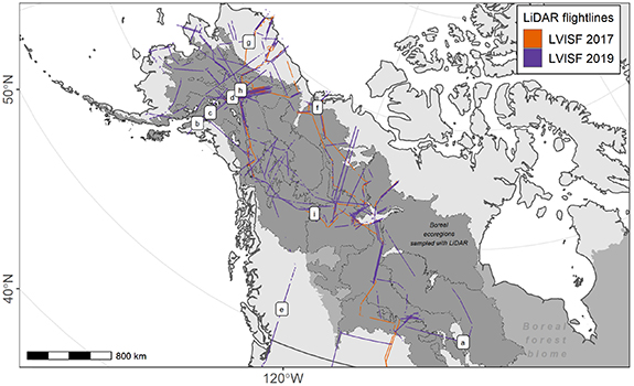
Figure 1. Map of LVISF 2017 and 2019 flightlines from the NASA ABoVE airborne campaigns across 15 boreal ecoregions in Alaska and Canada. The lettered locations shown correspond to sites along flightlines used as mapped examples of gridded estimates detailed below.
Download figure:
Standard image High-resolution image3. Data
3.1. Large footprint airborne waveform LiDAR
Large footprint airborne waveform LiDAR from LVIS sampled a broad boreal forest gradient in North America. These LiDAR waveforms were collected with a 1064 nm wavelength laser from the 'Facility' version of the LVIS instrument, in nominally 10 m diameter footprints with approximately 10 m spacing in both the along and across track directions. The flightlines from the 2017 campaign featured swath widths of nominally 1.8 km, while those from 2019 were 2.5 km. The waveforms for the footprints collected in these swaths were processed to a 'Level 2' as LVIS Facility L2 Geolocated Surface Elevation and Canopy Height Product (Version 1) (Blair and Hofton 2020) product and are available from the National Snow and Ice Data Center (NSIDC) via https://10.5067/VP7J20HJQISD.
3.2. Reference discrete return airborne LiDAR
Discrete return airborne LiDAR was used as reference estimates of boreal forest structure. These reference data were collected with NASA Goddard's LiDAR, Hyperspectral and Thermal (GLiHT) Imager (Cook et al 2013, Corp et al 2015) in the Alaskan growing seasons of 2014 and 2018. These data were acquired with a strip-sampling approach along flightlines with LiDAR pulse footprints of ∼10 cm in diameter. The 2014 acquisitions featured a pulse density of ∼4 m−2, while those from 2018 featured a pulse density of ∼12 m−2. For the forest structure captured in this dataset there were typically ∼2–3 LiDAR returns per pulse, resulting in an expected LiDAR return density of ∼8–12 LiDAR returns m−2 in 2014 and ∼24–36 LiDAR returns m−2 in 2018 (Montesano et al 2019).
3.3. Reference forest inventory data
We used plot-level disturbance data on time (in years) since the most recent disturbance from the Canadian National Forest Inventory (NFI) as reference for Landsat based stand age estimates (National Forest Inventory 2020). NFI data has been used widely to examine stand age (Girardin et al 2016, Besnard et al 2018, William et al 2018). The NFI's disturbance year recorded the most recent disturbance, which was used to calculate the number of years between the disturbance and the time of the base year for which age was being examined (2020). We included NFI plots with all disturbance types and mortality thresholds. The plot centroid (latitude, longitude) was used to extract corresponding Landsat stand age estimates for comparison of reference years since disturbance and remotely-sensed estimates of stand age.
3.4. Landsat stand age data
We used gridded 30 m estimates of stand age available as continuous maps across the boreal domain (Feng et al 2022). Stand age estimates were compiled using the methodology of identifying the year of the most recent disturbance in the Landsat time-series (Masek and James Collatz 2006). These estimates used a Landsat time-series record of yearly tree canopy cover from 1984 to 2020 that was calibrated to boreal forest structure. Breakpoint detection of disturbances identified the year of forest loss per pixel (assumed to be stand clearing). A forest establishment year was estimated based on the year in which regrown forest was first detected. This detection was based on the probability of a pixel being forest exceeding a threshold value for forest of 30% (Sexton et al 2013, Sexton et al 2015). The stand age of that pixel represents years since forest establishment of the current stand height estimate, calculated as the difference, in years, between this forest establishment year and the year of the height estimate from LVISF.
3.5. Climate data
We used climate data from WorldClim v2 (Fick and Hijmans 2017). These data were available as individual spatially referenced 1 km grids representing 19 bioclimatic variables spatially interpolated from weather station data across our study area.
4. Methods
4.1. Gridding footprint estimates of vegetation structure
Footprint estimates of vegetation structure summarize the vertically continuous LiDAR waveform. We acquired the latest version of these data (Version 1) from NSIDC as ASCII text files of individual flightlines. Natively, they feature a series of heights of canopy components at statistical percentiles recorded along the vertical distribution of LiDAR energy returned to the sensor. We used these native footprint height estimates to derive footprint-level vegetation canopy cover estimates, and gridded the suite of height and cover metrics.
Vegetation canopy cover provides useful horizontal structure context for estimates of vegetation's vertical structure. Estimates of vertical structure (e.g. canopy height) exist currently as standard attributes from Level 2 LVISF that are provided for footprint observations. To complement these vertical metrics of vegetation structure, we derived footprint-level estimates of vegetation canopy cover. For each footprint, the proportion of canopy cover for a given observation was calculated by subtracting from 1 the lowest relative height metric (a quantile value) whose height value exceeds a height threshold. For example, if the height threshold for canopy is 1.37 m and for a given observation the decile heights features RH30 = 1.2 m and RH40 = 1.5 m, then the proportion of canopy cover is 0.60. This result is based on an estimate of the proportion of the returned energy derived from above a specified height, all of which is assumed to be vegetation canopy. We produced estimates of cover using a variety of height thresholds, and used canopy cover estimates from a height threshold of 1.37 m for this study, a convention used across multiple studies to discern trees from shrubs. These estimates of cover are particularly useful for identifying height estimates that likely are not associated with forest or treed extents.
We then gridded footprint level estimates of vegetation structure. For each flightline, we used the ground latitude and longitude fields ('GLAT', 'GLON') to assign spatial coordinates to each footprint. Using the 'raster' package in R (version 3.6.1), we initialized an empty raster grid to 30 m resolution in the Canada Albers Equal Area Conic projection (EPSG:102 001) and used this empty raster as the base grid to which all other gridded data were aligned. The base grid was aligned to the ABoVE 30 m standard reference grid (Loboda et al 2019). The resolution of 30 m represents a trade-off between the higher spatial detail from individual footprints and continuous within-swath mapping of the gridded data for which areas with no-data values were significantly reduced. Here, the greater footprint spacing (lower density) of the 2019 campaign was the result of the higher flight altitude and faster speed during the acquisition.
For each canopy cover ('CC'), relative height ('rh'), vertical structure complexity ('COMPLEXITY') (Goetz et al 2010), and ground elevation estimate ('ZG') in each flightline, raster values were created by (1) specifying the extent and input resolution using the input footprint coordinates and the initialized grid, and (2) applying the rasterization function ('mean') to all footprints with centroids within a given grid cell. The rasterized data was exported as a 32-bit signed floating point value geotiff with a no-data flag value of 255. Similarly for each flightline, we calculated a grid of the count of contributing footprints ('count'), as well as grids for the associated 'min' and 'max' ZG estimates for each cell. The mapped and alphabetically labeled sites in figure 1 are detailed in figure 2, which shows examples from a variety of flightlines of individual footprints and the 30 m grid cell representing mean rh98 vegetation (canopy) height. Here, the variation of footprint density between flightlines is illustrated. The gridded versions of the LVIS L2 footprints are simplified summaries of multiple footprint estimates that coincide spatially within the same grid cell. Table 1 summarizes the full suite of grids produced for each LVIS flightline. Estimates of canopy cover were made for a suite of height thresholds.
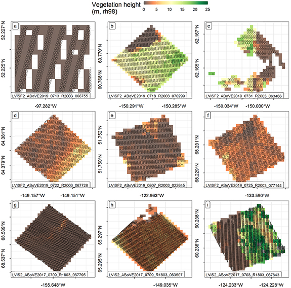
Figure 2. Examples of the mapped sites (shown in overview in figure 1) of LVISF footprint observations overlain atop corresponding gridded estimates representing the footprint mean of rh98 vegetation height. These maps depict a mix of forest structure and a variety of LiDAR footprint sampling to illustrate the effect of gridding footprints of various spatial densities. Each of the maps show the 10 m diameter LVISF footprint boundaries overlaid atop the 30 m gridded rh98 estimates.
Download figure:
Standard image High-resolution imageTable 1. A summary of the gridded Level 2 data. Each grid is named according to the following conventions: LVIS2_ABoVE < YYYY>_<MMDD>_<FLIGHTLINE>_<GRIDNAME>_<STAT>_30 m.tif.
| Name (GRIDNAME) | Rasterization function (STAT) | Description |
|---|---|---|
| lvis_pt_cnt | Count | The count of footprints whose centroids intersected the grid cell. |
| ZG | Min, mean, max | The ground surface elevation. |
| COMPLEXITY | Mean | The number of surfaces detected in the waveform |
| RH < metric_value> Metric_values: 010, 015, 020, 025, 030, 040, 045, 050, 055, 060, 065, 070, 075, 080, 085, 090, 095, 096, 097, 098, 099, 100 | Mean | Relative height percentiles of canopy surfaces above the ground |
| CC_gte_<height_threshold> m Height_thresholds: 00p20, 00p30, 00p50, 00p75, 01p00, 01p37, 01p50, 02p00, 03p00, 04p00, 05p00, 06p00, 07p00, 08p00, 09p00, 10p00, 12p00, 15p00 | Mean | The canopy cover estimate at a height greater than or equal to the specified height threshold (e.g. 01p37 = 1.37 m) |
4.2. Comparing gridded LVISF with reference discrete return LiDAR across a boreal gradient
To quantify the accuracy of LiDAR-derived stand height estimates across a range of boreal structure likely present across our regions of interest, the LVISF 2017 and 2019 acquisitions were compared to coincident (crossover) observations from legacy small footprint airborne LiDAR from GLiHT. Since these observations spanned the full boreal forest gradient in tree canopy cover, they provided valuable validation of the range of vegetation heights encountered across the broader study domain. The crossover locations where LVISF footprints coincide with GLiHT are found primarily in Alaska's Tanana and Matanuska-Susitna Valleys, with relatively few on the Kenai Peninsula (figure 3). These data, originally gridded as a canopy height model (CHM) at 1 m resolution, were resampled to the LVISF 30 m grids and converted to a suite of CHM relative height metrics (rhXCHM). These relative heights are those that are greater than X% of the set of 1 m CHM (reference top of canopy) pixels whose centroids fall within a given LVISF 30 m pixel. These rhXCHM values were used to examine the relationship of the many canopy height estimates from reference GLiHT with those from LVISF. The fractional cover estimate ('tree_fcover') from the suite of gridded GLiHT products was similarly resampled to provide canopy cover intervals for the comparisons. We note that there is a time difference between the LVISF and GLiHT observations of 1–5 years. We did not examine disturbed areas of these crossover locations and thus any disturbance that may have occurred at a crossover location between acquisitions will be part of the error associated with the model of LVISF and GLiHT heights.

Figure 3. Map of the set of LVISF and GLiHT LiDAR crossover locations within NASA's ABoVE study extent and the broader boreal domain.
Download figure:
Standard image High-resolution image4.3. Building a database of remotely sensed site history and current structure
The combination of forest site history and current structure provides key insights into forest productivity and growth. To assess one component of site history, we used reference plot data to validate Landsat-derived stand age estimates from a boreal-calibrated Landsat time-series of tree canopy cover (Sexton et al 2013, Sexton et al 2015, Feng et al 2022). To ascertain current structure, we used the gridded values representing the mean rh98 forest canopy heights as estimates of 'stand height'. Then, we built a database linking these stand heights from LVISF flightlines (n = 1887) to the corresponding Landsat-derived stand age estimates and 19 WorldClim v2 bioclimatic variables within boreal ecological regions (Olson et al 2001, Fick and Robert 2017).
We validated these Landsat-derived stand age estimates with reference NFI plots. For each plot in the domain for which Landsat age estimates were compiled (above 50°N) with a disturbance recorded (n = 120) we extracted the Landsat age estimates to each plot using its centroid. Then, we examined the correspondence between the Landsat age estimates and the years since disturbance referenced for each plot. These 120 plots were assigned one of four NFI plot classes that describe the nature of this correspondence. These classes stratify the relationship between the Landsat stand age estimate and the NFI years-since-disturbance into the following groups:
- 1.Invalid: disturbed since inventory: class for plots whose NFI age estimate is likely out-of-date because Landsat has indicated a disturbance at the plot more recently than the most recent NFI survey,
- 2.Landsat age >36: a flag class for plots where both NFI and Landsat did not indicate a disturbance within the Landsat record and thus there is no specific Landsat age estimate,
- 3.Landsat age >36; disturbance undetected: a flag class for plots where NFI indicates a disturbance within the Landsat record but Landsat does not, and thus there is no specific Landsat age estimate,
- 4.Landsat age estimate: class for plots where both NFI and Landsat indicate a disturbance within the Landsat record and thus there is a specific Landsat age estimate.
To build a database of height, age, and climate variables, we resampled the stand age and bioclimatic grids (nearest neighbor) to the 30 m LVISF grids and converted to a tabular format. We then extracted the ecoregion corresponding to each observation. This database was the basis for quantifying regional SI, which is the relationship of stand height with a given stand age for a specific ecoregion, an indicator of forest growth and productivity. Next, we filtered the database of stand height and stand age estimates to assemble gridded observations most useful for examining variations in SI across boreal ecoregions. We removed observations (1) with heights accrued at a rate >1 m yr−1, (2) from flightlines not intersecting boreal ecoregions, (3) corresponding to ecoregions not associated with landscapes featuring tree cover in general, (4) with LVISF tree canopy cover ⩽5% (using the LVISF threshold for canopy of height ⩾1.37 m), and (4) within ecoregions with fewer than 15 unique age values sampled. We then attributed each gridded height observation with an approximate stand age, returning a database of remotely sensed SI with n = 36 299 310 individual 30 m observations of stand height and stand age across the 15 boreal ecoregions covered in this study.
4.4. Quantifying regional SI
We used the database to quantify regional SI and assess patterns (the magnitude and variability) of boreal forest growth across environmental gradients. To quantify these growth rates we derived empirical models of SI (the variation of height with age). We assembled distributions from the remaining height observations from 1 year age class bins for each boreal ecoregion sampled, and calculated 3 per bin stand height quantile values (5th, 50th, and 95th percentiles) of these stand height distributions. We fit a non-linear model to each percentile, grouped by ecoregion, based on the Chapman–Richards forest growth equation (Pretzsch 2009), a negative exponential that is commonly used in a variety of forest growth studies (Besnard et al 2018). This model was fit for each ecoregion using the 'nlsList' function in the 'nlme' package of R, and was structured according to the form:
where  represent an individual pixel, height is mean forest stand canopy height based on rh98 (meters), age is the forest stand age based on the Landsat estimate of years since forest establishment,
  is the model asymptote (meters),
  is the model slope, and
  is the model inflection point representing the lag (years) associated with forest regeneration that occurs between the time of a disturbance and the onset of forest establishment. This parameter was held constant at 1 since the dependent variable age is an estimate of the actual year of forest establishment. The start parameters for the model fit were set as
  and
and  .
.
4.5. Assessing uncertainty in regional SI
We assessed the uncertainty of these ecoregion-specific SI models in two ways. We report both the prediction and confidence intervals from the non-linear models at the 95% level for each of the three predicted stand height quantiles for all corresponding stand age values available within each ecoregional sample of stand height and stand age using the predict_nls() function in the nlraa R package (Archontoulis and Miguez 2015, Miguez et al 2018, Miguez 2021). These uncertainties were calculated based on n = 1000 simulations of each ecoregion-specific SI model, and provide a rough estimate of the model error domain. The prediction intervals are relevant for examining the likely range of additional predictions of SI for individual stands or, potentially, tree observations. The confidence intervals are potentially more relevant as an estimate of the likely range of the mean from larger groups (populations) of many SI predictions. These two uncertainties provide flexibility for stochastic simulation of SI for both individuals and groups in a variety of forest growth models that operate across scales (from individual trees to broader landscape extents).
5. Results and discussion
5.1. Validation of estimates of stand height and stand age
We validated estimates of the two variables, stand height and stand age, used to quantify remotely sensed SI. Figure 4 shows the scatterplot densities along with the linear model results of relationships between coincident 30 m grid cell estimates from each sensor (LVISF and GLiHT) for each acquisition year, by 20% tree canopy cover intervals. The rh98 metric from LVISF was most similar to the rh90CHM metric (the 90th percentile of the set of reference top of canopy 1 m pixels) from GLiHT when gridded to match the LVISF 30 m grid. Relationships are weakest (R2 ⩽ 0.5) in the 20%–40% tree canopy cover intervals for the comparisons with 3 and 5 year differences between acquisitions (LVISF 2017 & GLiHT 2014 and LVIS 2019 & GLiHT 2014), and root mean square errors (RMSE) are largest (⩾1.9 m) for the 5 year difference comparison. Errors (RMSE) are lower from the comparisons with a 3 year time difference versus those with a 5 year difference, and feature fewer observations with near 0 LVISF canopy heights and GLiHT heights >5 m, an indication of the influence a time difference has on the LVISF height validation.
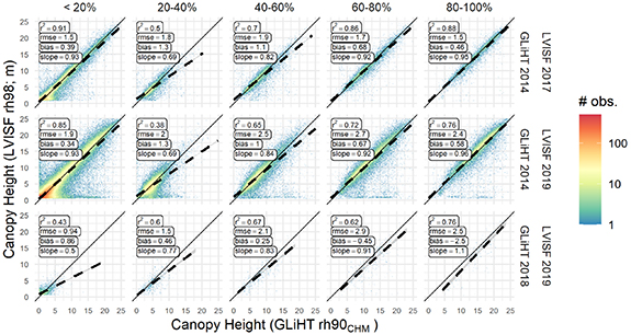
Figure 4. Boreal forest height estimates from LVISF rh98 at 30 m compared to coincident legacy GLiHT rh90CHM resampled to the same 30 m grid. The comparisons are made for each crossover between LVISF and GLiHT campaigns and are separated by tree canopy cover as defined by GLiHT, binned to 20% tree canopy cover intervals. Note: tree canopy cover interval labels are exclusive of the lower bound value.
Download figure:
Standard image High-resolution imageThe validation of Landsat stand age quantified the relationship of forest stand age estimates, derived from a time series of boreal tree canopy cover, with reference years since disturbance. Figure 5 summarizes key details of this validation. For 65 plots associated with the Landsat stand age values = 37, 22 plots featured disturbances indicated in the NFI data that were not detected in the Landsat time series. Of the NFI plots with Landsat stand age estimates from 0 to 36 years, 3 were invalid because Landsat detected a disturbance more recently than the measurement from the reference inventory. For the remaining plots in the class 'Landsat age estimate', we fit a linear model to assess the regeneration lag that accounts for the mean difference in the Landsat stand age estimates (years-since-establishment) and the NFI years-since-disturbance. The mean and standard deviation of differences (residuals) between the modeled relationship and Landsat stand age is 13.6 ± 5.4 years. This mean value provides an estimate of boreal forest establishment time, which is the years between a disturbance event and the point at which the forest stand (pixel) exceeds a threshold of 30% tree canopy cover. The standard deviation is an estimate of the variation in the time required for a forest to establish after a disturbance in the sampled areas of the boreal. This indicates that the Landsat stand age estimates used to assess regional growth patterns begin, on average, nearly 14 years after a recorded disturbance in which forest loss was detected. These results complement ground studies that report on boreal seedling establishment (3–10 years post-fire) (Johnstone et al 2004), which precedes the estimate of forest or stand establishment considered in this study. This validation demonstrates the use of a time series of tree canopy cover to describe a key detail of site history, and thus the relevance of these data for remote sensing studies of forest growth.
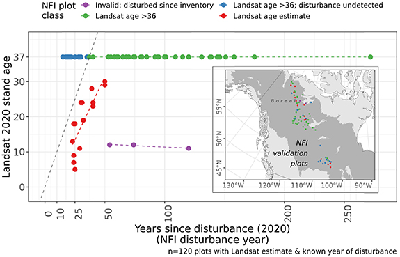
Figure 5. The validation scatterplot for the four classes of NFI validation plots (n = 120) with Landsat stand age estimates (Feng et al 2022) used to examine variation in regional SI patterns. NFI validation plots shown in red feature estimates of stand age from disturbances occurring within the Landsat time series 1984–2020 and provide a relationship between the remotely sensed stand age and reference years-since-disturbance. The identity line (Landsat stand age = years-since-disturbance) is represented with a black dashed line. The inset map shows the spatial distribution within the boreal domain (dark gray area) of these NFI validation plots.
Download figure:
Standard image High-resolution image5.2. Empirical models of SI for boreal ecoregions
Figure 6(A) depicts the models for each of the three percentiles of stand height for each ecoregion along with the corresponding SI35 value, which represents the number of years covered between this study's age estimates (1984; the start of the Landsat time-series record used) and the most recent LiDAR height estimates (2019). Figure 6(B) sorts the ecoregions by 95th percentile height, from greatest to least to highlight our estimate of the relative differences in regional productivity potential across the study domain, and figure 6(C) shows bars corresponding to the number of 30 m pixel observations from each region used in these SI models. The calculations of stand height growth rates are summarized for the 15 boreal ecoregions in figure 6(D). These rates at the three stand height percentiles are summarized for 4 years along a stand development timeline using the growth equations shown in figure 6(A). These 4 years correspond with SI10 , SI35 , SI50, and SI100.
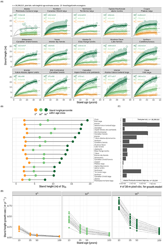
Figure 6. The magnitude and variability of stand height with age across 15 boreal ecoregions in North America from central Canada westward across Alaska. (A) Non-linear models fit by ecoregion to the 5th, 50th, and 95th percentiles of the stand height distributions within each 1 year age class. Colored circles correspond to the stand height percentile value for the corresponding stand age. SI model uncertainty is captured with confidence and prediction intervals, shown with dark (tighter) and light (broader) colored ribbons, respectively, around the fitted model curves (black dashed lines). Subplot text annotations show predicted SI35 values and the corresponding standard deviation of residuals for each of the 3 percentile SI models. (B) An ecoregion comparison of the three percentiles of SI35 highlights regional variability in height distributions for stands after 35 years of growth, and (C) bar plots compare the number of height and age samples analyzed for each ecoregion listed in (B). (D) Stand height growth rates (m yr−1) for the 15 boreal ecoregions at the 3 stand height percentiles computed for 4 years along the stand development timeline using the growth equations modeled in (A). These 4 years correspond with stages of stand development during a projected 100 year period; an early stage (SI10), a young stage at the end of the Landsat time-series (SI35), an intermediate stage after half a century (SI50), and a mature stage after a century (SI100).
Download figure:
Standard image High-resolution imageFigure 7 summarizes the ecoregion variation in height potential and its uncertainty. These maps show the predicted SI mean (figure 7(a)), and standard error (figure 7(b)), its 95% confidence interval (figure 7(c)), and the model sigma (standard deviation of the residuals; figure 7(d)), using the upper stand height percentile value at 35 years ( ) for each of the 15 boreal ecoregions of this study. This approximates the growth rates of the tallest stand heights present in these ecoregions after 35 years, potentially representing sites with favorable growth conditions. We note the most poorly sampled ecoregion 'Alaska Peninsula montane taiga' features n = 664 observations for stand ages 10–20 and n = 0 observations for stand ages <10, which results in an SI95th model with uncertainties well exceeding the magnitude of their means, and therefore are not plotted.
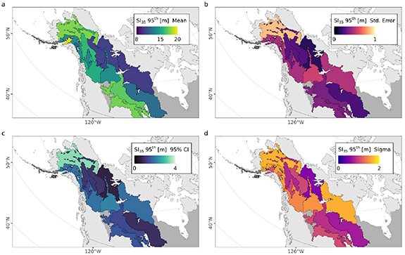
Figure 7. An approximation of regional boreal forest productivity potential and variability from SI and its uncertainty at a stand age of 35 years. Mapped SI35 shows the 95th quantile value of (a) mean, (b) standard error, (c) 95th percentile confidence interval, and (d) SI model sigma (standard deviation of the residuals) of stand height at a stand age of 35 years for each of the boreal ecoregions with samples of height and age observations.
Download figure:
Standard image High-resolution image5.3. Changes in explained variation for relationship of regional SI and bioclimatic drivers
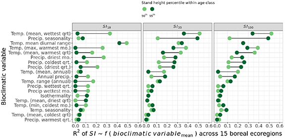
The relationship of SI with key bioclimatic drivers of forest growth changes across a stand development timeline. We examined the relationship of the median (50th) and upper (95th) SI10, SI35, and SI100 values from all 15 boreal ecoregions in this study to regional means of broad-scale bioclimatic variables from WorldClim v2 (Fick and Robert 2017) (figure 8). The linear model R2 from these relationships indicates the proportion of variation in SI across the 15 boreal ecoregions that is explained by the corresponding mean ecoregion bioclimatic value. Figure 8 highlights differences between bioclimatic drivers of SI along a stand development timeline, showing R2 results at three stages during this projected 100 year period; an early stage (SI10), the end of the Landsat time-series (SI35), and after a century (SI100). The change in the R2 values at different stages of growth shows the variation in the strength of these drivers of growth (both median and upper percentile growth cohorts) projected across a 100 year period of boreal forest growth. This summary indicates which broad-scale bioclimatic drivers of growth may be most relevant during early, middle, and late stages of stand development, suggesting the stage-dependent nature of the importance of these drivers on stand growth. Forest and ecosystem growth models may modify the constraints imposed upon growth from these drivers of boreal forest productivity according to the stage-dependence of their importance.
Figure 8. The relationship of SI with drivers of forest growth. Linear model R2 results from the set SI values of 15 boreal ecoregions with corresponding mean ecoregion bioclimatic values show variation in the drivers of growth associated with median (50th) and upper (95th) percentile site indices for forest growth occurring early (SI10), after a period the length of the Landsat time-series (SI35), and after a century (SI100).
Download figure:
Standard image High-resolution image
5.4. Relevance of regional SI for boreal forest and ecosystem modeling
These results reduce two large archives of remote sensing data (airborne LiDAR and Landsat) to provide a foundation for incorporating direct estimates of SI and forest growth variation across multiple ecological regions into boreal forest and ecosystem models. For these regions, the SI models can be used in three important ways to explore forest demography and its variation. This is critical for updating the manner in which forest and ecosystem models operate within and across boreal ecoregions (Leonardo and Poulter 2021).
First, these regional SI models can update existing equations that constrain the model parameters in high resolution gap modeling frameworks (Kruse et al 2016 , Foster et al 2017 ) for handling the growth of individual trees across a range of vegetation types and sites through time. Often, gap models use general equations that provide an initial constraint for capturing growth relationships and then rely on environmental thresholds and competitive interactions to constrain and modify growth. These remote sensing derived observations offer a spatially-explicit approximation of forest growth rates, where variation captured between the lower (5th) and upper (95th) percentiles of SI may bound growth across all vegetation demographics within a given ecoregion, itself a representation of distinct biota nested within a biogeographic realm (Olson et al 2001). These bounds can help explore the diversity of likely trajectories for boreal forests experiencing changing composition, structure, and fire regimes.
Second, these empirical SI models can improve how physical forest growth models account for vegetation heterogeneity. Applied back to the continuous maps of stand age, these SI models provide a means to map how SI varies across smaller scales. This is important for models operating at all scales in regions where abrupt spatial patterns in vegetation may be a key feature associated with landscape dynamics (e.g. the taiga-tundra ecotone; Montesano et al 2021). Furthermore, patterns of productivity linked to successional-stage provide an opportunity for models to improve accounting of recovery from disturbances. Coarser models, e.g. Lund-Potsdam-Jena Wald, Schnee, Landschaft version 2.0 (LPJwsl v2.0; Leonardo and Poulter 2021), can benefit from updated areal proportions with particular growth rates, while high-resolution models can incorporate the mapped heterogeneity directly, and explore how growth varies with other local scale factors such as hydrology, topography, soils, and forest composition.
Finally, these SI models can be used to evaluate SI from spaceborne observations of vegetation structure. Due to greater spatial coverage spaceborne-derived SI (e.g. from combining vegetation structure measurements from ICESat-2 or NISAR with the Landsat time-series-derived age estimates) can then be used to extend SI across the full boreal domain in much greater detail. This potential for full domain scaling would help both quantify SI across smaller landscape spatial scales and extend modeling opportunities with spatially explicit SI to most or all landscapes in the boreal domain. Significant portions of the boreal forest, particularly in permafrost larch forests, have so far remained out of reach of openly available LiDAR estimates such as those used for this study. Calibrating the spaceborne LiDAR estimates of boreal forests using the relationship of coincident ICESat-2 and LVISF observations will support more routine efforts for evaluating patterns of growth and recovery across, for example, disturbed forests from various levels of burn severity. Furthermore, quantifying SI across smaller landscapes and PFTs would enhance the site-scale relevance, enabling analysis of local scale drivers of growth, and modeling with continuous mapped estimates that vary by pixel.
5.5. Limitations of regional SI estimates from archives of airborne LiDAR and Landsat
The large archive of LVIS LiDAR samples and three decades of the Landsat time-series produced >36 million gridded SI estimates for this study. Yet, estimates from the use of one of the most comprehensive airborne vegetation height datasets across a broad boreal extent is not without its limitations.
There are inherent limitations in these regional SI models that generalize forest growth across ecoregion extents. While the boundaries likely do not impose undue error on our methods, as plant vegetation adheres to sharp polygon boundaries, thus supporting ecoregionalization as a useful technique for summarizing vegetation properties (Smith et al 2018, Martins et al 2022), there remains a significant loss of understanding of vegetation patterns on the landscape. Still, the results capture growth dynamics within areas of similar biogeography and climate, and reproduce a gradient of growth that is consistent with widely recognized forest structure and environmental gradients in the North American boreal domain (Brandt 2009). Each model aggregates growth across many site conditions that include variations from topography, plant functional type, soil characteristics, and disturbance return intervals. However, they entangle the variation imposed by microsite differences. As such, these models do not represent trajectories of growth for any single vegetation demographic, rather, their uncertainty bounds suggest a range in which regional growth may vary.
Regionalization was critical for this study. It provided the key to unlock the power of the massive LiDAR sampling across an extent for which we use continuous gridded maps of stand age estimates (Feng et al 2022). It allowed us to perform an uncertainty analysis that is tailored to some types of modeling studies. The methodology used in this study is not the only way of working with these data. Another study could certainly derive per-pixel estimates of SI using corresponding height and age pixel values (as we did as an intermediate step), and stop at mapping SI per pixel within flightlines. Recognizing the biogeographic value of a statistical summary from merging multiple flightlines, we grouped these estimates by ecoregions because we see a particular downstream modeling use-case whereby these growth equations and their uncertainties are used to constrain modeling studies of growth relevant for sites within the bounds of the ecoregions whose growth rates we summarize. A number of studies highlight the importance of accounting for regional variation when quantifying SI (Karlsson 2000, Bontemps and Duplat 2012, Bontemps and Bouriaud 2014). However, the trade-off in spatial detail means that these results are not appropriate for sub-regional studies of growth without additional site information.
6. Conclusions
We quantified the magnitude, variability, and uncertainty in region patterns of SI by linking airborne LiDAR samples of current forest structure estimates with Landsat stand age estimates across 15 boreal ecoregions in North America. These regional SI patterns can be used to parameterize simulations from high resolution forest growth models for simulation sites spread across a broad spatial extent in the North American boreal forest. Inherent limitations exists with regional SI summaries for understanding site-specific growth dynamics, yet results provide a foundation for incorporating large volumes of direct estimates of vegetation structure and growth into ecosystem models. As part of this work we produced an open archive of a gridded version of the current forest structure estimates, including relative height metrics, vertical canopy complexity, and ground elevations, from the LVIS Facility L2 Geolocated Surface Elevation and Canopy Height Product (Version 1) at 30 m spatial resolution, and computed a variety of tree canopy cover estimates from this suite of data. Finally, we validated an open archive map of boreal forest stand age to calculate a remote sensing estimate of stand establishment in years to demonstrate the relevance of stand age for remote sensing forest growth studies.
Acknowledgments
Funding for this work was provided through NASA solicitations NNH16ZDA001N-CARBON, NNH18ZDA001N-TE. We thank the NASA ABoVE Science Team and the ABoVE Vegetation Structure Working Group for input into the LVIS dataset preparation. We acknowledge the prerequisite work of airborne flight campaign planning performed by the ABoVE Science Team, and its execution, and raw and level 1 dataset processing performed by the NASA Goddard Space Flight Center LVIS Team. The high performance computational resources for the gridding of the Level 2 LVIS data was provided by the ADAPT system at the NASA Goddard Center for Climate Simulation. We appreciate the help of Byron Smiley of Natural Resources Canada for assistance acquiring the forest inventory data.
Data availability statement
The suite of gridded boreal forest structure data used in this study is the first of its kind openly available to evaluate boreal forest patterns at local scales across structural gradients that span broad geographic extents. Gridded data have been archived at the Oak Ridge National Laboratory Distributed Active Archive Center along with the R code used to rasterize the LVIS Level-2 ASCII text files (10.3334/ORNLDAAC/1923; Montesano et al 2021). Two tables used to report SI are available upon request. These are:
- 1.The regional quantile-specific SI model summary table, which includes SI model coefficients, SI predictions for SI10, SI35, SI50, & SI100, and their associated standard errors, SI 95% confidence and 95% prediction intervals.
- 2.The SI prediction table of predicted quantile stand heights, by region, for each input stand age value, which includes the 95% confidence and prediction bands around each predicted value.
Authors' contributions
PM conceived the study design, performed the analysis, and wrote the manuscript. CN, LD, AA, JS and CM helped with the study design and provided manuscript feedback. MM derived the canopy cover estimates, compiled LVIS processing scripts and helped process the gridded LVIS data, and PW compiled and provided access to the stand age data. WW helped extract spaceborne data to airborne observations.
Conflict of interest
The authors declare that they have no conflicts of interests.
df_lvis_smry_updated.csv The SI prediction table of quantile stand heights (0.3 MB CSV)
Supplementary data (<0.1 MB DOCX)
SI_all_join.csv The summary table of SI model predictions (<0.1 MB CSV)