
Abstract
The influence of pulse length, working gas pressure, and peak discharge current density on the deposition rate and ionised flux fraction in high power impulse magnetron sputtering discharges of copper is investigated experimentally using a charge-selective (electrically biasable) magnetically shielded quartz crystal microbalance (or ionmeter). The large explored parameter space covers both common process conditions and extreme cases. The measured ionised flux fraction for copper is found to be in the range from ≈10% to 80%, and to increase with increasing peak discharge current density up to a maximum at , before abruptly falling off at even higher current density values. Low working gas pressure is shown to be beneficial in terms of both ionised flux fraction and deposition rate fraction. For example, decreasing the working gas pressure from 1.0 Pa to 0.5 Pa leads on average to an increase of the ionised flux fraction by percentage points (pp) and of the deposition rate fraction by taking into account all the investigated pulse lengths.


Original content from this work may be used under the terms of the Creative Commons Attribution 4.0 license. Any further distribution of this work must maintain attribution to the author(s) and the title of the work, journal citation and DOI.
1. Introduction
Magnetron sputtering [1, 2] is a physical vapour deposition (PVD) technique [3], in which ions are accelerated from a plasma, whose density is significantly increased by the presence of a static magnetic field, towards a cathode target. Under the ion bombardment, target material is ejected from the cathode in a process called sputtering to then condense on a substrate, forming a thin film. The sputtered particles predominantly enter the discharge as neutral atoms, however ions and even clusters of atoms have also been reported to be present in the sputtered flux [4, p 552]. PVD, and magnetron sputtering especially, plays a key role in the manufacturing of integrated circuits, where it is appreciated for its relative simplicity, high-deposition rate, and low cost, and is used for depositing functional metal thin films [5, 6]. In particular, PVD processes find extensive use in interconnect metallisation at various scales, from connecting individual devices in the back-end-of-line (BEOL) [5] to connecting different dies with through-silicon-vias (TSV) [7–9] in 3D integration.
Due to its low bulk resistivity (), relatively high melting temperature (), and good electromigration resistance [10], Cu is commonly the material of choice for realising these electrical connections, which consist of trenches and vias with aspect-ratios ranging from on average 1:6 in the Cu damascene BEOL process [11] up to 1:10 or even more for some TSV applications. A high net directionality of the film-forming material is essential to ensure good step- or sidewall-coverage and void free filling of such high aspect-ratio structures [6, 12]. This can be achieved by ionising the sputtered atoms and accelerating the ions towards the wafer, e.g. using substrate biasing [13]. For an acceleration potential significantly higher than the ion thermal energy, the ions will arrive with a narrow velocity distribution centred around the normal direction. If the fraction of ions in the flux of target metal atoms reaching the substrate, termed the ionised flux fraction, is sufficiently large, the deposition will be predominantly directional.

One approach to obtain such a highly ionised flux is high-power impulse magnetron sputtering (HiPIMS), a variation of magnetron sputtering where high power pulses are applied to the cathode target with a low duty cycle (0.5%–5%) [14, 15]. The high pulse power results in an increased plasma density and thus higher ionisation of the film-forming species. Early demonstrations of the HiPIMS technique used discharges with a Cu target, which showed very promising results including void free filling of 1:1.2 trenches [16–18]. In one of these first studies on HiPIMS deposition of Cu [18], the ionised flux fraction was reported to be about 70%—the accuracy of this measurement has however since been questioned [19]. For other target materials, such as Ti, Al, and Ni, the ionised flux fraction has been found to be in the range 10%–60% and to increase with increased discharge current density [20], but it is known to also depend on other parameters such as the working gas pressure or the magnetic field strength [21–23].

Besides the benefit of increased directionality, a high ionised flux fraction also enables tuning of the energy of the charged deposition flux using, for example, substrate biasing, which can enhance various film properties. Indeed, increased ionised flux fraction leads to increased mass density of the deposited films, as has been demonstrated for a number of elemental metallic films [24]. Furthermore, an increased ionisation of the film-forming material in the HiPIMS process has been shown to be beneficial for the film microstructure and for tailoring internal stress during growth [25–27], and for achieving low electrical resistivity in Cu thin films [28].
While the lining or filling of trenches and vias often requires pushing the ionised flux fraction to the maximum [6], it should also be noted that for best film performance this is not always desirable. For example, Ross et al [29] found that an increased ionisation in HiPIMS deposition of Ti also favoured the formation of multiply charged Ti ions (e.g. Ti2+) at the expense of singly charged ions (Ti+), which is known to induce high compressive stress in compound thin film materials [30]. This highlights the need for being able to tune the ionised flux fraction using accessible (external) process parameters.
Additionally, increasing the ionised flux fraction usually comes at the cost of further reducing the deposition rate fraction—a phenomenon which has been dubbed the HiPIMS compromise by Brenning et al [31]. It has been suggested that a HiPIMS discharge can be optimised in this regard by selecting appropriate operating parameters, including working gas pressure [31], pulse length [32], and waveform [33]. Knowledge of how the choice of these process parameters influences the deposition rate and the amount of deposited ions can be used as a guide when tailoring the deposition for a particular application and greatly facilitate the optimisation process.
The aim of the present work is to accurately determine the ionised flux fraction of Cu in HiPIMS and compare it with earlier reports, and, more importantly, to extend our understanding of how to optimise these discharges by systematically exploring the available parameter space and establish not only trends regarding individual parameters, but also shed light on the interplay of the different effects. To this end, the deposition rate and ionised flux fraction have been measured for HiPIMS discharges of Cu as the working gas pressure (), the pulse width (), and the peak discharge current () were varied simultaneously.

The experimental setup, measurement method, and general methodology used for that purpose are explained in section 2. The measurement results are presented and analysed in section 3, which is then followed by a discussion of the observed trends in section 4. Finally, the key findings are summarised in section 5.
2. Methodology
2.1. Experimental apparatus
The measurements were performed in a cylindrical stainless steel deposition chamber, in diameter and in height, which was equipped with a 152 mm diameter and 6.4 mm thick Cu target mounted on a standard, unbalanced, planar magnetron assembly. The base pressure was maintained at or below Pa by a Pfeiffer Vacuum (DN250) TMH 1601 P C H turbomolecular pump.


The argon (99.9997% purity) working gas pressure was measured using an MKS 626D Baratron capacitance manometer and calibrated before each discharge by regulating the mass flow in the range of 73 sccm–570 sccm.
The discharges were ignited by an HiPSTER 6 Ionautics HiPIMS pulser unit driven by a Technix SR series 6 kW 1 kV HV dc generator and either triggered internally or externally using an Agilent Technologies 33210A arbitrary wave-form generator. The target voltage and discharge current waveforms were recorded using a PicoScope 4444 20 MHz digital oscilloscope connected to the respective probe outputs of the HiPIMS pulser unit. The average discharge power was calculated by integrating the instantaneous power over a duration of 1 s according to
where is the discharge voltage and the discharge current.


In order to maintain a constant average power of 500 W while varying the pulse length, working gas pressure, and peak discharge current density, the pulse repetition frequency was adjusted in the range of 19–1170 Hz. This large range is due to the large variation in average pulse energies (0.42–26 J) from cases at the extreme ends of the explored parameter space. The average power was chosen as low as possible in order to minimise target erosion over the course of the study while still achieving stable discharges for the low repetition rate cases.
The deposition rates were determined as a fraction of the rate measured for a reference direct current magnetron sputtering (dcMS) discharge as explained in section 2.2. When operating in dcMS mode, the dc power supply unit otherwise used to drive the HiPIMS pulser was directly connected to the magnetron assembly instead, and the power was set to 500 W by adjusting the discharge voltage.
2.2. Ionised and total flux measurements
The metal ion content in the film-forming flux and the total deposition rate are commonly quantified using the dimensionless ionised flux fraction and deposition rate fraction defined as


and
where and are respectively the total deposition rate and the total deposition rate for a reference dcMS discharge operated at the same average power and otherwise identical conditions, and and are the deposition rates due to ions and neutrals only, respectively [31, 34]. As can be seen from the definitions in equations (2) and (3), being ratios, these quantities are independent of the absolute deposition rates and thus average power. This facilitates comparisons and has the advantage of not requiring an absolute rate calibration.


The total as well as neutral deposition rates required for the computation of the ionised flux and deposition rate fractions were measured using a magnetically shielded, charge-selective quartz crystal microbalance (QCM), henceforth referred to as ionmeter, as described by Kubart et al [21]. Such electrostatically [35] or magnetically shielded [36] QCM-based devices have previously been employed to measure the degree of ionisation of the sputtered metal flux in ionised PVD (iPVD). In particular, ionmeters have been used to characterise HiPIMS discharges of, amongst others, Al, Ti and Cu [22, 37, 38], and more recently to experimentally determine the angular dependence of the deposition rates due to ions and neutrals in HiPIMS discharges of Ti [39].
The ionmeter was set up at a typical substrate position, at a distance of from the target surface and directly facing the ionisation region (and target racetrack) as illustrated in figure 1. It was protected by a shutter when not in use and at the beginning as well as the end of a measurement. The bias required for the neutral rate measurements was supplied by an OLTRONIX B60-5 R dc power supply connected over a 500 Ω resistor. The bias voltage, nominally set to , and the current drawn by the QCM were monitored using a Tektronix P2220 voltage probe and a Chauvin Arnoux C160 current clamp, both connected to the PicoScope 4444 unit also used to record the discharge current and voltage. Gold-coated AT-cut quartz crystals with a base frequency of 6 MHz were used down to a minimum of 57.5% crystal life, and the film thickness was registered using a Kurt J Lesker FTM-2400 readout unit (film mass density , Z-factor Z = 0.44).


Figure 1. Illustration of the ionmeter and its placement with respect to the target (not to scale). The dashed line on the right-hand side represents the vertical axis going through the centre of the target. The core of the ionmeter is a quartz crystal microbalance (QCM). Magnets are placed on top of the unit to create a local magnetic field which prevents the electrons from reaching the biased top electrode of the quartz crystal.
Download figure:
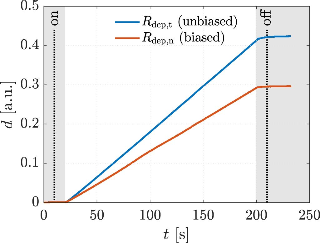
Standard image High-resolution imageTo make the measurements more robust against eventual noise, all measurements followed the exact same procedure. The recording of the crystal frequency was started with the shutter still closed and the pulser unit turned off. After 10 s, the pulser unit was turned on, and after yet another 10 s, the shutter was opened. After a measurement duration of, depending on the deposition rate, 180–600 s, the shutter was closed, and after yet another 10 s, the discharge was turned off again. Finally, the recording was stopped after at least another 20 s had passed. The rate could then be calculated by comparing the frequency before and after the deposition. An example of such a rate measurement is shown in figure 2. The individual rates have also been normalised with respect to the average power to account for small deviations from the 500 W set point.

Figure 2. An example of a rate measurement illustrating the measurement procedure. The plot shows the thickness d in arbitrary units (a.u.) measured by the QCM as function of time. For the total rate measurement (unbiased, blue line) the top electrode of the crystal is grounded and for the neutral rate measurement (biased, red line) a bias of was applied. The shutter was in the closed position in the shaded areas, and the moments at which the pulser unit is turned on or off are marked with dotted lines. The amount of noise in the measurement varies significantly depending on the discharge conditions and the procedure has been chosen with that in mind.


Download figure:
Standard image High-resolution image2.3. Experimental design
The bulk of the experiments were performed in three main blocks, starting off with a Box–Behnken-like design (block I) with the variables (working gas pressure), (pulse length) and (peak discharge current density), which was first extended to a full-factorial-like design (block II), and then again to higher pressures (block III) for a total of investigated discharges. The levels for the pulse length were chosen equidistant, ranging from to , while for the working gas pressure , a logarithmic scale ranging from 0.25 Pa to 2 Pa was used. Since the maximum reachable peak discharge current density depends on the former two variables, a nominal scale (low, medium, high) ranging from to was applied for the peak discharge current density to nevertheless be able to explore high peak discharge current scenarios.


In an attempt to minimise systematic errors that might arise due to, e.g. target erosion [40], crystal usage or chamber and crystal heating over the course of the large number of measurements, the experiments in each block were performed in a randomised order. Additionally, the setup was not modified and vacuum never broken during these three phases. An overview of the complete measurement plan can be found in table 1.
Table 1. The process and flux parameters of the 36 main experiments listed. The experiment numbers reflect the order the experiments have been performed in.
| — | (Pa) | () | (A) | (V) | (Hz) | (%) | (%) |
|---|---|---|---|---|---|---|---|
| 7 | 0.25 | 25 | 90 | 870 | 580 | 38 | 21 |
| 6 | 0.25 | 50 | 90 | 750 | 360 | 42 | 22 |
| 1 | 0.25 | 50 | 180 | 865 | 145 | 29 | 62 |
| 4 | 0.25 | 75 | 180 | 830 | 94 | 29 | 64 |
| 10 | 0.50 | 25 | 90 | 810 | 605 | 38 | 15 |
| 3 | 0.50 | 25 | 180 | 935 | 250 | 18 | 39 |
| 8 | 0.50 | 50 | 180 | 820 | 130 | 22 | 47 |
| 11 | 0.50 | 75 | 180 | 795 | 77 | 24 | 59 |
| 9 | 0.50 | 75 | 270 | 1000 | 34 | 20 | 65 |
| 13 | 1.00 | 25 | 180 | 880 | 255 | 16 | 25 |
| 12 | 1.00 | 50 | 180 | 780 | 126 | 17 | 31 |
| 2 | 1.00 | 50 | 270 | 960 | 55 | 8 | 62 |
| 5 | 1.00 | 75 | 225 | 870 | 45 | 15 | 69 |
| 15 | 0.25 | 25 | 45 | 750 | 1130 | 54 | 11 |
| 17 | 0.25 | 25 | 135 | 940 | 360 | 31 | 48 |
| 19 | 0.25 | 50 | 135 | 800 | 220 | 32 | 39 |
| 27 | 0.25 | 75 | 135 | 745 | 170 | 35 | 38 |
| 26 | 0.25 | 75 | 225 | 930 | 55 | 27 | 81 |
| 25 | 0.50 | 25 | 135 | 875 | 375 | 28 | 31 |
| 14 | 0.50 | 50 | 135 | 750 | 200 | 27 | 26 |
| 18 | 0.50 | 50 | 225 | 905 | 80 | 18 | 68 |
| 22 | 0.50 | 75 | 225 | 905 | 47 | 23 | 73 |
| 24 | 1.00 | 25 | 135 | 820 | 385 | 25 | 22 |
| 16 | 1.00 | 25 | 225 | 950 | 180 | 11 | 33 |
| 23 | 1.00 | 50 | 225 | 860 | 82 | 12 | 56 |
| 20 | 1.00 | 75 | 180 | 760 | 73 | 19 | 48 |
| 21 | 1.00 | 75 | 270 | 960 | 33 | 14 | 66 |
| 33 | 2.00 | 25 | 180 | 838 | 262 | 13 | 17 |
| 32 | 2.00 | 25 | 225 | 900 | 187 | 8 | 18 |
| 34 | 2.00 | 25 | 270 | 970 | 140 | 7 | 32 |
| 30 | 2.00 | 50 | 180 | 740 | 130 | 13 | 21 |
| 35 | 2.00 | 50 | 225 | 816 | 85 | 10 | 49 |
| 36 | 2.00 | 50 | 270 | 892 | 59 | 8 | 77 |
| 29 | 2.00 | 75 | 180 | 725 | 74 | 12 | 22 |
| 31 | 2.00 | 75 | 225 | 810 | 48 | 8 | 46 |
| 28 | 2.00 | 75 | 270 | 900 | 33 | 6 | 46 |


Additional measurements extending the Pa cases to higher peak discharge current densities and longer pulse lengths, repetitions of previous measurements, and measurements at were carried out later on to confirm trends seen in the previous measurements. It should however be noted, that by the time these measurements were performed, the setup had undergone some changes and the target had been significantly eroded (erosion depth of 1.8 mm corresponding to a little less than one-third of the target thickness). These measured values are displayed in appendix

3. Results
The discharge voltage and current waveforms for the investigated discharges are shown in figure 3 and the discharge parameters as well as the measured ionised flux fractions and deposition rate fractions are summarised in table 1 and visualised in appendix

Figure 3. The discharge voltage and current waveforms for the main measurements listed in table 1 (i.e. without the additional measurements) averaged over 32 samples each and grouped by pressure and pulse length. The three different colours correspond to different pulse lengths—25 µs in blue, 50 µs in red, and 75 µs in yellow—and this colour scheme is kept throughout the manuscript. To distinguish the different waveforms, those with lower peak discharge current are shown in a darker colour.
Download figure:
Standard image High-resolution imageTwo observations stand out right away. First, ionised flux fractions above 80% have been measured ( at , Pa, ), confirming that it is indeed possible to attain values as high as reported in the disputed measurements by Kouznetsov et al [18] ( at , Pa, , using the same discharge chamber as in this current study but with a different pulser unit). Second, the spread in both and are enormous—ranging from roughly 10% to 80% and 5% to 55%, respectively. These large ranges of achievable flux parameters are a result of the large parameter space available in HiPIMS operation, which stresses the importance of process optimisation [31, 33].


In an attempt to provide guidance for this task and separate the effects of working gas pressure, peak discharge current density, and pulse length, the deposition rate and ionised flux fractions are successively analysed by looking at how their values change compared to a reference discharge at typical HiPIMS conditions ( Pa, ). This then also allows quantifying and comparing the influence of each of these external parameters.


3.1. Deposition rate fraction
The measured deposition rate fraction is visualised by the symbols in figures 4(a)–(c) grouped by pulse length. Fitted surfaces, obtained as described below, are included as an aid for localising the points. There is a clear decreasing trend with both increasing working gas pressure and increasing peak discharge current density. The fitted surfaces should however not be used to extrapolate to values outside the region delimited by the measured points.

Figure 4. The measured deposition rate fraction (symbols) together with the fitted response surfaces (mesh) for (a) 25 , (b) 50 , and (c) 75 long pulses. The meshes show lines of constant and . The direction of the peak current density axis is reversed to allow for a better view. The reference discharge = 1 Pa) is marked with the corresponding measured value.


Download figure:
Standard image High-resolution imageIn order to quantitatively analyse the influence of the process parameters, the variation in the measured deposition rate fraction is formally decomposed into effects due to changes in the working gas pressure and peak discharge current density according to


where A00, A10, A20, and A01 are fitting parameters used to estimate and quantify the individual effects and do not have a direct physical meaning. To facilitate the interpretation of the results, the recentred and dimensionless variables and /(1 Pa) have been introduced, where the offsets have been chosen such that corresponds to the chosen reference discharge. Thanks to this change of variables, the fitting parameters have a relatively straightforward meaning. For instance, simply corresponds to the estimated value for the chosen reference discharge at Pa () and () since both and are trivially equal to zero:


Similarly, A01 corresponds to the change associated with changing the working gas pressure by a factor of two, since for example at we have and thus

or at ()


Finally, the change associated with increasing or decreasing the peak discharge current density by with respect to the chosen reference peak discharge current density of is given by the sum ()


respectively the difference ()


of A20 and A10.
Using equation (4) it is now possible to fit response surfaces to the measured values. The fitted surfaces, obtained using an ordinary least squares regression on the main measurements, are illustrated in figure 4. The individual changes in percentage points (pp) on the deposition rate fraction by changing the working gas pressure or the discharge current density are plotted in figures 5(a) and (b), respectively. The corresponding parameter values as well as the root-mean-square error (RMSE) are shown in figure 6.


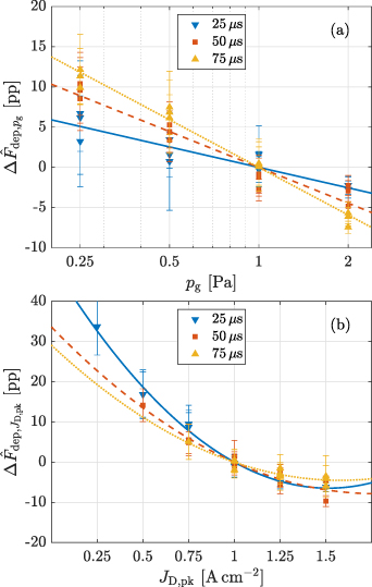
Figure 5. The effects of (a) working gas pressure and (b) peak discharge current density on the deposition rate fraction for the 25 , 50 , and 75 long pulses. Also shown are the measured values with the remaining terms in equation (4) subtracted.


Download figure:
Standard image High-resolution image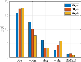
Figure 6. The values of the deposition rate fitting parameters obtained for the 25 , 50 , and 75 long pulses. The normalisation is chosen such that the values of A10 and A20 correspond to a change of 0.5 A cm−2 with respect to the reference peak current density (1 A cm−2), and the value of A01 to a reduction of the working gas pressure by a factor of two with respect to the reference pressure (1 Pa). Note that signs for A10 and A01 have been inverted to simplify comparisons.


Download figure:
Standard image High-resolution imageAs can be seen in figures 5(a) and (b), the fits accurately reproduce the measured deposition rate fraction to within a margin of without the need for an interaction term, indicating that the effects of peak discharge current density and working gas pressure are well separable. At the chosen reference point of and Pa, the deposition rate fraction is in the range 16%–18% (see figure 6) showing comparatively little variation between the three pulse lengths. Both increasing peak discharge current density and increasing pressure have a negative effect on the deposition rate fraction. Figure 5(a) suggests decreases linearly with the logarithm of the pressure, a reduction by a factor of two corresponding to, depending on pulse length, an increase of 3 pp–6 pp, and that the pressure effect is stronger for longer pulses, as can also clearly be seen by the increasing value of in figure 6. The effect of increasing peak current density, visualised in figure 5(b), is negative and can be well approximated by a second order polynomial. The effect is strongest for the 25 pulses and decreases with increasing pulse length. A decrease of the peak discharge current density by 0.5 A cm−2 to () leads to an increase in the range of and an increase by 0.5 A cm−2 to () to a decrease in the range of , highlighting that the deposition rate penality is initially high but diminishes as the peak current density is increased further. This can also be seen when looking at the steepness of the curves in figure 5(b).


3.2. Ionised flux fraction
The measured ionised flux fraction is shown in figures 7(a)–(c) grouped by pulse length, again together with fitted surfaces to serve as a visual aid. Generally, there is an increasing trend with increasing and a decreasing trend with increasing . However, the situation is much less clear than for the deposition rate fraction. Therefore, splitting the change into different effects in a similar fashion to equation (4) proves especially helpful


where again and /(1 Pa), and where B00, B10, B20, B01, and B11 are fitting parameters. The addition of an interaction term () was necessary to be able to approximate the measurements with reasonable accuracy. In consequence, the interpretation of the parameter values is unfortunately less straightforward. This can be somewhat remedied by considering to be a correction to B10 as suggested in equation (5). The resulting response surfaces are shown in figures 7(a)–(c). The main effects related to working gas pressure and peak discharge current density are displayed in figures 8(a) and (b), which also show that all measurement points lie within of the fitted values. Compared to the deposition rate, the deviations are noticeably larger. This is to be expected due to both the larger range of values and inherently larger uncertainty associated with the measurement of compared to .


Figure 7. The measured ionised flux fraction (symbols) together with the fitted response surfaces for (a) 25 , (b) 50 , and (c) 75 long pulses. The meshes show lines of constant and . The direction of the working gas pressure axis is reversed to allow for a better view. The reference discharge Pa) is marked with the corresponding measured value.


Download figure:
Standard image High-resolution image
Figure 8. The effects of (a) peak current density and (b) working gas pressure on the ionised flux fraction for the 25 , 50 , and 75 long pulses. Also shown are the measured values (symbols) with the remaining terms in equation (5) subtracted.


Download figure:
Standard image High-resolution imageThe strength of the individual effects are compared in figure 9. At the reference point (, Pa), the ionised flux fraction is typically in the range to 41% and increases with increased pulse length. The decrease associated with an increase in pressure by a factor two is roughly the same across the different pulse lengths at to . There is a strong increase with increased and the changes are much more pronounced for the 50 and 75 pulses as indicated by the corresponding bars of B10 and B20 in figure 9. Increasing the peak discharge current density from the reference point (, Pa) by 0.5 A cm−2 to () leads to an increase of pp to 36 pp while a decrease by the same amount down to () results in a reduction by to . At this point, it should be noted that extrapolation to low peak current densities is problematic and instead a dcMS-like behaviour where generally is close to zero, as reported elsewhere [23], should be assumed. The negative value of B20 indicates diminishing returns or even slight decreases at the high end, which again is more pronounced for the 50 and 75 pulses. Finally, the values of B11 tell us, that, while for the 25 pulses the effect of changing the peak current density is approximately independent of pressure, the associated variation is larger at higher pressures for the longer pulses.


Figure 9. The values of the fitting parameters obtained for the 25 , 50 , and 75 long pulses. The normalisation is chosen such that the values of B10 and B20 correspond to a change of 0.5 A cm−2 with respect to the reference peak current density (1 A cm−2), and the value of B01 to a reduction of the working gas pressure by a factor of two with respect to the reference pressure (1 Pa). The value of B11 can be interpreted as a pressure dependent change in the linear peak discharge current effect B10. Note that signs for B20 and B01 have been inverted to simplify comparisons.


Download figure:
Standard image High-resolution image4. Discussion
4.1. Comparison to earlier works
There have been a number of studies of the plasma parameters of a HiPIMS discharge with a copper target, including Langmuir probe studies that report on the electron density and electron energy [41–43], and mass spectrometry studies to determine the ion flux and ion energy [44–46]. In particular, Vlček et al [45] demonstrated that the Cu+ ions can dominate the ion flux and reported that Cu+ ions constitute up to 92% of the total ion flux onto the substrate. The ionisation region model (IRM) has been applied to model HiPIMS discharges with a copper target [38]. These studies confirmed that the discharges are dominated by self-sputter recycling [47] at high discharge currents, and that the ion flux into the diffusion region is dominated by Cu+ ions (i.e. ). This agrees with the fact that gas-less self-sputtering from a copper target in a HiPIMS discharge has been achieved [48, 49] using a vacuum-arc discharge to ignite the discharge at a background gas pressure of 10−3 Pa. These reports indicate that should be high for at least some HiPIMS discharge conditions, but not how and the deposition rate change.


While the authors are not aware of any systematic investigations of how the deposition rate and ionised flux fraction are influenced by the external process parameters in HiPIMS discharges of copper, some work has previously been done for other material systems.
In their investigation of HiPIMS discharges of Al and Ti at different working gas pressures ({0.5 Pa, 2 Pa}), and for different pulse lengths (), Lundin et al [22] found ionised flux fractions in the range of 23%–78% and 23%–65%, for Al and Ti, respectively, while varying the average pulse discharge current density in the range of 0.5 A cm−2 to 2 A cm−2. For Al, depending on the chosen pressure and pulse length, they reported an increase of 16 pp to 26 pp when going from around 0.5 A cm−2 to 1 A cm−2. In the corresponding Ti discharges, the increase was slightly lower or 10 pp to 22 pp, which corresponds to a relative increase of about 35%–80%. The difference between the average pulse discharge current density used in the earlier study by Lundin et al [22] and the peak discharge current density can however be quite large (see e.g. Butler et al [34]), which complicates the comparison somewhat. For reference, while the peak discharge current densities explored in the present study range from 0.25 A cm−2 to 1.5 A cm−2, the corresponding average pulse discharge current densities were considerably lower or in the range from 0.1 A cm−2 to 1.2 A cm−2.

A more direct comparison can be made with the measurements on Ti HiPIMS discharges by Shimizu et al [37] carried out in the same deposition chamber and using the same magnetron assembly as used for this work. They varied the peak dicharge current density and the pulse length while keeping the average power constant. For pulse lengths between 25 and 75 and at a working gas pressure of Pa, their data shows an increase of the ionised flux fraction in the order of 8 pp–14 pp and a decrease of the deposition rate fraction in the range of −8 pp to −11 pp when increasing the peak discharge current density by 0.5 A cm−2. Furthermore, the changes of both and are larger for shorter pulse lengths. For the 25 pulses, a one-to-one comparison can be made by interpolating the values found for copper to the peak discharge current densities and working gas pressure used in the work by Shimizu et al, as shown in figures 10(a) and (b). At Pa, the corresponding increase in ionised flux fraction is in the range of 27 pp to 35 pp and decrease in deposition rate fraction in the range of −11 pp to −19 pp. As such, the effects are noticeably larger for copper than for Ti.


Figure 10. Comparison of (a) the deposition rate fraction and (b) ionised flux fraction in HiPIMS discharges of Ti (blank) and Cu (filled) at otherwise identical conditions ( Pa). The values for Ti are taken from Shimizu et al [37] and the values for Cu have been obtained from the measurements in the present work using equations (4) and (5). In subplot (b), only two, respectively one, points are shown for the 50 and 75 Cu discharges, since the ionised flux fraction can not reasonably be extrapolated to low peak current densities.


Download figure:
Standard image High-resolution imageShimizu et al [37] also noted a decrease in both deposition rate and ionised flux fraction when the pulse length was increased. This is not supported by the presented findings. However, it should be noted that the pulse lengths investigated in the present work are rather short. Conversely, if one were to look only at the Ti discharge with pulse lengths between 25 to 75 , no obvious trend would be noticeable either for the cases with and . In fact, the range from 25 to 75 has deliberately been chosen for the present work, exactly because it corresponds to the deposition rate maximum for Ti observed by Shimizu et al [37], and because both and were expected to decrease when increasing the pulse length—which is confirmed by the additional measurements at 100 and 150 shown in appendix


4.2. Influence of the external discharge parameters
While there are no clear direct trends regarding the pulse length in the investigated range, there are notable differences in how the discharges with shorter (25 ) and the longer (50 and 75 ) pulses are affected by changes in the other process parameters. Looking at the discharge current waveforms in figure 3, what distinguishes the short pulses is that they are all triangular. For the longer pulses, the shapes vary more and the discharge current waveform can no longer be described simply by the peak discharge current and the pulse width. In consequence, the response surfaces seen in figure 7 are more complex.


The effect of increasing the peak discharge current observed herein is, on the other hand, much clearer and in accordance with expectations. The material pathways model [51, 52], which is briefly described in appendix


Let us now turn to the effect of the working gas pressure. That lower pressure can be beneficial has previously been suggested by Lundin et al [22], and more recently been supported by measurements of the angular distribution of the neutral and ion fluxes in Ti HiPIMS discharges by Renner et al [39] at different working gas pressures. The present results confirm that reduced pressure increases both the ionised flux fraction and the deposition rate fraction. As seen in section 3, the influence of on both and takes in fact a rather simple form, while, however, at the same time eluding a simple explanation in terms of the material pathways model. The estimates in appendix


4.3. Decrease in ionised flux fraction at high peak discharge current densities
The response surface of the ionised flux fraction for the 75 pulses shown in figure 7(c) suggests a decrease at peak discharge current densities above , which is not seen for the shorter pulse lengths investigated. This is not just an artefact due to fitting with a quadratic function. The ionised flux fraction measured for the discharges at are indeed consistently lower than those measured for the at otherwise identical conditions. Later measurements at and again , displayed in figure B.12, show with one exception also all lower ionised flux fractions than the discharge at the same pressure. It should be noted, however, that by the time these measurements were performed the target had been significantly eroded and the setup had undergone some changes. A similar unexpected decrease at high peak discharge current densities has already been observed in previous measurements, which were performed to obtain ionised flux fraction for locking the IRM [38] and are included in the supplementary data.


One possible reason for this unexpected trend could be due to limitations of the ionmeter. As illustrated in figure 1, the QCM is biased across a 500 Ω resistor and in consequence a large bias current can introduce a significant voltage drop. During the present measurements, the bias voltage was monitored and was observed to reach values as low as 20 V during the afterglow in some cases. However, under the assumption that the portion of high energy ions () in the afterglow is comparatively small, this would still not explain the significant decreases in .


Assuming that this effect is indeed real, another possible explanation can be found in the shape of the discharge current waveform. Lower ionised flux fractions for the 1.5 A cm−2 than for the 1.25 A cm−2 discharges have been observed for the 75 pulses at 0.5 Pa, 1.0 Pa, and 1.5 Pa which all have in common that the discharge current maximum occurs much earlier than the end of the pulse (see figure 3). Since during the pulse a lot of ions are recycled and the amount of ions released in the afterglow is mainly determined by the current density at the end of the pulse, this could negatively impact the ionised flux fraction [32].

One of the motivations for this study was the observation of this unexpected decrease in ionised flux fraction at high peak discharge current densities in previous, less systematic, measurements shown in the supplementary data. For this work, the bias voltage applied to the ionmeter has been monitored and overloading of the bias power supply can be excluded as the cause. However, it is still not possible to say with certainty that the observed effect is real. To this end, a follow-up study which, in addition to different direct methods (e.g., retarding field energy analyser (RFEA), gridded QCM), uses an indirect method to qualitatively judge the metal ion content in the film-forming flux, for example by measuring the coverage of vias or trenches in biased substrates, could be used to confirm this effect. Additionally, the deposited films could also be used to link the observed changes in ionised flux fraction and deposition rate to film properties. In particular, it can be expected that there will be an increase in compressive film stress at low pressure, which could introduce further optimisation constraints depending on the application [55].
5. Conclusion
In order to facilitate optimisation and improve our understanding of HiPIMS of copper in an argon atmosphere, a detailed map of the external process parameter space covering both most commonly used process points as well as more extreme cases has been produced.
To this end, the deposition rate and ionised flux fractions in copper HiPIMS discharges have been measured over a wide range of process parameters and fitted using a polynomial model. Both fractions have been found to linearly increase with the negative logarithm of the pressure, meaning that low working gas pressure is beneficial for both of these quantities. Furthermore, the pressure and peak discharge current dependencies of the deposition rate fraction have been found to be well separable, meaning that the increase in deposition rate fraction gained by decreasing the pressure is approximately independent of the peak discharge current density. In the explored range, the dependence of the ionised flux fraction and the deposition rate fraction on the peak discharge current density is well described by a second order polynomial, where the overall effect of increasing is generally positive for and negative for .


In the more extreme cases, very high ionised flux fractions above 80% have been observed, confirming that previously questioned values as described by Kouznetzov et al [18] are indeed attainable. Furthermore, the expected and well known trend of increasing ionised flux fraction with increasing peak discharge current density has been shown, however a new and surprising decrease at very high peak discharge currents has been observed as well.
While the possibility of this effect not being real but rather the result of an issue with the measurement apparatus or method cannot be excluded at this point, possible next steps to confirm these unexpected results have been proposed.
The presented data set also offers a great opportunity to more closely investigate the inner workings of the Cu HiPIMS discharge using computational methods such as the IRM, which can use the measured values as a model constraint, in order to properly explain the observed effects.

Additional open questions that could be addressed in future work are how well these results can be generalised and to what extent they depend on the geometry and the magnetic field strength and topology.
Acknowledgments
This work was partially funded by the Swedish Research Council (Grant No. VR 2018-04139), the Swedish Government Strategic Research Area in Materials Science on Functional Materials at Linköping University (Faculty Grant SFO-Mat-LiU No. 2009-00971), the Icelandic Research Fund (Grant No. 196141), and Evatec AG.
Data availability statement
All data that support the findings of this study are included within the article (and any supplementary files).
Conflict of interest
The authors have no conflicts of interest to disclose.
CRediT
Joel Fischer: conceptualisation, investigation, methodology, formal analysis, visualisation, writing—original draft, writing—review & editing. Max Renner: investigation, writing—review & editing. Jon Tomas Gudmundsson: writing—review & editing. Nils Brenning: writing—review & editing. Martin Rudolph: writing—review & editing. Hamid Hajihoseini: writing—review & editing. Daniel Lundin: supervision, funding acquisition, resources, formal analysis, writing—review & editing.
Appendix A: The material pathways model
The material pathways model was first introduced to explain the reduction in deposition rate in the HiPIMS process [51] and later applied to directly estimate the ionised flux fraction in discharges where the pulses were sufficiently long to reach a steady state [52]. In the present work, an updated version of the model which allows for direct comparisons with dcMS discharges [56] is used. The two most important parameters are the target atom ionisation probability αt, which describes the likelihood of a sputtered atom being ionised, and the target ion back-attraction probability βt, which is the likelihood that an ionised target ion cannot escape the cathode potential fall and is accelerated back to the target. Since the spatial distribution of ions and neutrals is generally not the same, an additional parameter , the ratio of the neutral and ion transport parameters [57], is needed to describe the ionised flux fraction [56]
and the sputter rate normalised deposition rate fraction
From a practical point of view, is of lesser interest and, unlike the deposition rate fraction , also experimentally not easily accessible. To get from to , the relative differences in the sputter rate and the neutral transport parameter between HiPIMS and the corresponding (same pressure and average power) dcMS discharge need to be taken into account as well:


While the target atom ionisation probability αt and the target ion back-attraction probability βt might not be interesting for the deposition process itself, they create a link to the discharge physics and thus the process parameters [31]. They are experimentally not readily accessible, but can be estimated from the measured ionised flux fraction and deposition rate fraction by inverting equations (A.1)–(A.3) to give the target atom ionisation probability


and the back-attraction probability
where
and
where and are the discharge voltages for the corresponding HiPIMS and dcMS discharges, respectively, and where the fraction of the ion current at the target surface that is carried by Ar+ ions is


The assumed values for the transport parameter ratios
and
are taken from Rudolph et al [56].
For a detailed explanation of the different quantities, please refer to the original publication outlining this procedure [56]. The values for the sputter yields and were taken from Anders [58] and are the same as used in the IRM code [38]. The present estimate differs slightly from Rudolph et al [56]. Since the peak discharge current density and working gas pressure vary over a large range, instead of assuming a constant value, the working gas ion current contribution ζ was allowed to vary. It was taken to be proportional to the ratio of the maximum current that could be carried by argon ions [59] and the peak discharge current . The value of the proportionality constant in equation (A.8) was set to . However, it can be noted that the value of has little influence on αt and βt, since the sputter yields of copper and argon are relatively close in the investigated voltage range. For reference, the maximum relative difference between calculated with and is below 10%.


The ionisation probability obtained from the measurement data using this approach is displayed in figure A.11. Over the investigated range of peak discharge current densities, the estimated value of αt increases from around 60% at 0.25 A cm−2 to close to 100% at 1.5 A cm−2, and depends little on parameters other than the peak discharge current density, even though and , which were used to compute , both show non-trivial dependencies on the working gas pressure and pulse length.


Figure A.11. The ionisation probability αt for the investigated discharges as calculated according to equation (A.4) (symbols). Different working gas pressures are not distinguished using different symbols. Also shown are a fit of the form proposed by Rudolph et al [20] (solid line) and a second order polynomial fit (dotted line).
Download figure:
Standard image High-resolution imageAppendix B: Measurement data
The ionised flux fractions and deposition rate fraction for all investigated discharges, including the additional measurements that were performed later on, are displayed in figures B.12 and B.13, respectively. Plots showing the separate total and neutral rates used to compute and have been included in the supplementary data.


Figure B.12. The measured ionised flux fraction as a function of the peak discharge current density grouped by pulse width (in ) for working gas pressure of (a) 0.25 Pa, (b) 0.5 Pa, (c) 1 Pa, and (d) 2 Pa. Blank symbols correspond to repeated or additional measurements.


Download figure:
Standard image High-resolution image
Figure B.13. The measured deposition rate fraction (normalised to the dcMS discharge at the same average power and the same respective pressure) as a function of the peak discharge current density grouped by pulse width (in ) for working gas pressure of (a) 0.25 Pa, (b) 0.5 Pa, (c) 1 Pa, and (d) 2 Pa. Blank symbols correspond to repeated or additional measurements.


Download figure:
Standard image High-resolution image
Footnotes
- 7
For a description of the transport parameters and the normalised sputter yield, please refer to appendix A.