
Abstract
The possibility to optimize a high-power impulse magnetron sputtering (HiPIMS) discharge through mixing two different power levels in the pulse pattern is investigated. Standard HiPIMS pulses are used to create the ions of the film-forming material. After each HiPIMS pulse an off-time follows, during which no voltage (or, optionally, a reversed voltage) is applied, letting the remaining ions in the magnetic trap escape towards the substrate. After these off-times, a long second pulse with lower amplitude, in the dc magnetron sputtering range, is applied. During this pulse, which is continued up to the following HiPIMS pulse, mainly neutrals of the film-forming material are produced. This pulse pattern makes it possible to achieve separate optimization of the ion production, and of the neutral atom production, that constitute the film-forming flux to the substrate. The optimization process is thereby separated into two sub-problems. The first sub-problem concerns minimizing the energy cost for ion production, and the second sub-problem deals with how to best split a given allowed discharge power between ion production and neutral production. The optimum power split is decided by the lowest ionized flux fraction that gives the desired film properties for a specific application. For the first sub-problem we describe a method where optimization is achieved by the selection of five process parameters: the HiPIMS pulse amplitude, the HiPIMS pulse length, the off-time, the working gas pressure, and the magnetic field strength. For the second sub-problem, the splitting of power between ion and neutral production, optimization is achieved by the selection of the values of two remaining process parameters, the HiPIMS pulse repetition frequency and the discharge voltage of the low-power pulse.
Export citation and abstract BibTeX RIS

Original content from this work may be used under the terms of the Creative Commons Attribution 4.0 licence. Any further distribution of this work must maintain attribution to the author(s) and the title of the work, journal citation and DOI.
1. Introduction
The dc magnetron sputtering (dcMS) discharge is typically operated at a cathode voltage of a few hundred volts and discharge current densities in the range of 4–60 mA cm−2 which result in power densities of a few tens of W cm−2. The degree of ionization is very low resulting in a deposition flux composed of mainly neutral atoms and the majority of ions bombarding the substrate are ions of the noble working gas [1]. In high-power impulse magnetron sputtering (HiPIMS), a high ionized flux fraction in the deposition flux onto a substrate is achieved by short pulses of high power, which are applied to a standard magnetron sputtering device [2, 3]. The peak power densities are >500 W cm−2 and the peak discharge current densities are commonly >0.5 A cm−2. The significant ionization of the deposition flux results in a number of desirable properties of the produced thin films, as reviewed in a few different works [4–7], but it comes at the cost of a reduction in deposition rate to typically 30%–85% of the dcMS rates, when depositing at the same average power [8]. The loss in deposition rate depends strongly on the target material [8]. However, it also depends on other process parameters including the working gas pressure, the magnetic field strength, the HiPIMS pulse amplitude and the HiPIMS pulse length [9–15]. A problem is that increasing the deposition rate quite often leads to a lower ionized flux fraction of the sputtered material [14, 16, 17], i.e., by partly sacrificing the initial reason to use HiPIMS instead of dcMS. For this reason, a high deposition rate, taken alone, is not a suitable criterion for the quality and/or optimization of a HiPIMS discharge. Also the ionized flux fraction is needed to give the complete picture [18].
The present work builds on a recent study by Brenning et al [18], herein called paper I, on how to optimize HiPIMS discharges in a way that takes into consideration both the ionized flux fraction and the deposition rate. Paper I describes the optimization of conventional HiPIMS discharges generated by isolated high amplitude pulses, during which both the ions and the atoms in the flux to the substrate are created. We will here extend the study to a more advanced pulse pattern, involving also a dcMS-like stage of the discharge, which opens the possibility to create ions and neutrals in different time windows. The approach of combining a pulse of high power density with a dcMS discharge dates back to the earliest reports on high-power pulsed magnetron sputtering discharges, which were then referred to as high-current low-pressure quasi-stationary discharges in a magnetic field [19, 20]. There a high-power pulse was superimposed onto a dcMS discharge that maintains the discharge between the pulses. This is now referred to as pre-ionized HiPIMS [21–23], which involves maintaining a low-power dc discharge (voltage below 300 V and a discharges current of a few mA) that provides seed charge at the beginning of the HiPIMS pulse and ensures a faster rise of the discharge current when the high-power pulse is applied.
As a suitable background to the present work, we will first briefly review how optimization of conventional HiPIMS discharges to maximize the deposition rate was treated in paper I for any given combination of ionized flux fraction and average discharge power. To this purpose the Ti/Ar system was used as an example. Datasets from multiple experimental HiPIMS studies were combined with computational modelling of the internal discharge plasma chemistry using the ionization region model (IRM) [24]. The deposition rates and the ionized flux fractions were then determined as functions of four experimental process parameters: the HiPIMS pulse length tHiP, the HiPIMS peak discharge current IHiP, the working gas pressure pgas, and the magnetic field strength, quantified as the magnetic field strength Brt at the racetrack center. In paper I it was concluded that the three parameters Brt, pgas and tHiP should be minimized, each as far as being compatible with the choice of the two others and with the need to ignite the discharge. The fourth parameter IHiP was reserved for choosing the optimum balance between a high ionized flux fraction and a high deposition rate, referred to as the HiPIMS compromise, which is based on the idea that a fully ionized material flux is not necessarily needed to achieve significant improvement of the (application-dependent) thin film properties [25]. In this aspect, a sufficiently high IHiP was required to reach the desired ionized flux fraction. Further increase of IHiP would lead to unnecessarily low deposition rates.
With the more advanced pulse pattern presented here, the average discharge current during the HiPIMS pulse 〈IHiP〉 becomes available as an additional free parameter for optimization. This work explores the possible gains through this extra degree of freedom. The pulse pattern suggested here is shown in figure 1. Standard HiPIMS pulses are used to create the ions of the film-forming material. After each HiPIMS pulse an off-time follows, during which no voltage (or, optionally, a reversed voltage, such as used in bipolar HiPIMS [26–29]) is applied, letting the remaining ions in the magnetic trap escape towards the substrate. Applying a reversed positive voltage pulse to the sputter target, right after the high-power negative sputter pulse, turns the target into an anode that when positively biased increases the plasma potential and thereby provides a knob to control the ion bombarding energy towards the growing film [28, 29] but does not influence the sputter process. After these off-times, a long second pulse at lower voltage and discharge current amplitudes, in the dcMS range, is applied. During this pulse, which is continued up to the following HiPIMS pulse, mainly neutrals of the film-forming species are produced. This pulse pattern makes it possible to maximize the efficiency of the ion production, during the HiPIMS pulses, independent of the choice of the optimum ionized flux fraction.
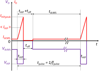
Figure 1. A pulse pattern showing the time-evolution of the discharge voltage, and the discharge current, where the production of ions and neutral fluxes to the substrate is separated in time, and therefore can be optimized independently. The figure also defines the process parameters VHiP, 〈IHiP〉, VdcMS, IdcMS, tHiP, toff and tpulse = 1/fpulse. The HiPIMS discharge current waveforms are here given a triangular form, which is commonly observed for short pulses, as those proposed in this work.
Download figure:
Standard image High-resolution imageThe whole optimization process thus becomes separable into two sub-problems, which are addressed in section 2. Section 2.1 describes the first sub-problem concerning the minimization of the energy cost for putting ions onto the substrate. This means choosing the optimum values of a first set of process parameters: Brt, pgas, tHiP, toff, and 〈IHiP〉. The second sub-problem is treated in section 2.2, which deals with making the HiPIMS compromise between the ionized flux fraction and the deposition rate, and describes an optimization method to determine the two remaining process parameters fpulse and VdcMS. Section 3 contains a discussion of the results by working through a numerical example, and section 4 contains a summary and conclusions. Details of the modeling referred to in this work are given in the appendix
2. Theory and observations
2.1. Sub-problem 1: minimizing the cost of ionization
We will here proceed in two steps. First, in section 2.1.1, the energy cost per ion from the HiPIMS pulses that is deposited onto the substrate,  ti,HiP, is expressed as a function of three dimensionless internal parameters which we take from the materials pathway model as summarized by Gudmundsson et al [3], namely αt, βt and ξt, where αt is the ionization probability of sputtered target species, βt is the fraction of these ions that return to the target (back-attraction probability), and the transport parameter ξt [30] is the fraction of the remaining ion flux of target species which is deposited onto the substrate. From the latter definition it also follows that the fraction
  of the ion flux of target species from the ionization region (IR) to the diffusion region is lost to the chamber walls. Then, in section 2.1.2, a process flow chart model is used to analyze the influence routes as follows: from the process parameters Brt, pgas, tHiP, toff, and 〈IHiP〉, through the internal parameters αt, βt and ξt, and finally to the figure of merit
  . This will provide insight into how to vary the process parameters in order to minimize
  .
.
2.1.1. A figure of merit for the HiPIMS pulses
The first goal is to derive an expression for the energy cost per ion of the film-forming species that is deposited onto the substrate. Ions of the sputtered target species are here assumed to be produced only within the dense plasma (the IR) that is maintained during the HiPIMS pulses. The total electric energy delivered to the discharge during one pulse is

where the HiPIMS power source is assumed to keep the voltage VHiP constant throughout the pulse and the integration is taken over the HiPIMS pulse only. To simplify, we will now also assume that 〈IHiP〉 is given by the total ion current at the target surface, neglecting the small contribution from secondary electrons [24, 31]. Note that this approach applies to an arbitrary discharge current waveform.
We also need to estimate the number of ions, of the target species, that are deposited onto the substrate from each HiPIMS pulse. These originate as atoms, sputtered by ions bombarding the target during a pulse, that are subsequently ionized. The total number of ions bombarding the target during a pulse is 〈IHiP〉tpulse/e, with e being the elementary charge. As a simplification, we here assume that the ions are only singly charged. In a HiPIMS pulse the effective sputter yield depends on the ion composition in the ion current onto the target. Following Hajihoseini et al [14], we define ζ to be the working gas fraction of these ions and (1 − ζ) the sputtered species fraction. In our case, with Ar working gas and a Ti target, we have an effective sputter yield Ysput,eff per ion given by

where the indices are such that Ar+ → Ti denotes Ar+ as the bombarding ion species and Ti as the target material and Ti+ → Ti denotes self-sputtering of the target. The number of sputtered atoms per HiPIMS pulse is then

A fraction αt of this number becomes ionized, and of these ions a fraction βt is back-attracted to the target. Consequently the number of target species ions per pulse that enters the diffusion region, where the substrate is placed, is Nsput,HiP αt(1 − βt). The number of ions that is finally deposited onto the substrate per HiPIMS pulse becomes

where ξt is the transport parameter as defined above. The energy cost per target species ion that is deposited onto the substrate is obtained by combining equations (1)–(4) to give

where WE,HiP is the electric energy delivered to the HiPIMS pulse as a whole, i.e., it also includes for example the energy used to produce the neutral flux component. All of this energy is necessary for the pulse even if we are focusing on the ions—and therefore, for simplicity, we refer to  as the 'energy cost' for the ions. For ion energies typical for magnetron sputtering discharges we can make the simplification that the sputter yields are approximately proportional to the square root of the ion energy [32–34]. We further assume that most of the applied potential falls over the cathode sheath, so that the ion energies are proportional to VHiP. The sputter yields can then be written as

for sputtering by the working gas ions and for self-sputtering

where  and
and  are material-dependent coefficients specific to these two ion/target combinations. Combining equations (2), (6) and (7) gives
where Ksput,eff is the effective sputter yield coefficient

Combining equations (5) and (8) finally gives

This is the figure of merit, which gives the energy per ion of the film-forming material deposited onto the substrate. A discharge that is arranged so that  is minimized will deliver ions to the substrate at the lowest possible energy cost per ion. We can note here that this expression contains only one external parameter, VHiP, which is easily obtained in a studied discharge. The remaining four parameters αt, βt, ξt and Ksput,eff are internal to the discharge, and more difficult to assess. Tuning of αt and βt using accessible process parameters will be explored in the next section, while the parameters ξt and Ksput,eff are addressed in section 3.
2.1.2. A flow chart analysis of the process parameters
The optimization task can, at this step, be formally identified as minimizing  . In practice, however, it is not obvious how to go about this. What we have available to vary in an experiment are not the internal discharge parameters in equation (10), but a set of external process parameters. Of these, we will in this section discuss five. Two of those parameters refer to the discharge setup, Brt and pgas, and the remaining three parameters define a HiPIMS pulse of the type shown in figure 1: tHiP, toff, and
  ; the more elaborate notation
  is here used for 〈IHiP〉 since we, in connection with this figure, will discuss how 〈IHiP〉 is selected by varying VHiP. The question is how these five parameters influence the variables in the expression on the right-hand side of equation (10).
Figure 2 shows a flow chart model, of a type earlier used in paper I, which gives a simplified overview of the network of mechanisms that are involved in the HiPIMS deposition process. The left column contains the external process parameters that can be varied, and the right column contains the figure of merit that is to be minimized. The middle column contains the two internal discharge parameters αt and βt. The arrows denote the mechanisms through which one parameter influences another parameter, and their color indicates the type of influence. A green (filled) arrow marks a co-correlation, i.e., an increase of the parameter at the start of a green arrow gives an increase in the parameter at the tip, and a decrease gives a decrease. A red (unfilled) arrow marks the opposite, a counter-correlation.
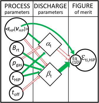
Figure 2. A flow chart that shows the main influences from the external process parameters (left column), through internal processes represented by the parameters αt
and βt
(middle column), and finally to the figure of merit  (right column), which is to be minimized. Green (filled) arrows mark a co-correlation and red (unfilled) arrows mark a counter-correlation as described in the text.
Download figure:
Standard image High-resolution imageWe will first go through the arrows one by one, and then discuss their interplay. We start with the three arrows on the right in the figure, those which end up at the figure of merit  . These three arrows are determined by equation (10) and are generic in the sense that they hold for any HiPIMS discharge, not only the Ti/Ar system studied here.
Influence
 . The pulse voltage VHiP is not an independent process parameter but used to obtain the desired discharge pulse current. This is the reason for the notation 〈IHiP(VHiP)〉 in figure 2. However, a change in VHiP also leads to a change in the sputter yield. The energy scaling of the sputter yield in equation (8) is such that it gives the proportionality
  in equation (10). An increase in VHiP thus gives an increase in
  , and we here get a green (filled) arrow.
Influence
 . According to equation (10) an increase in αt gives a decrease in
  by the same factor. Please note that no physics is involved here. This relation follows directly from the definition of the ionization probability αt. We get a red (unfilled) arrow.
Influence
 . In equation (10) an increase in βt gives a decrease of the factor
  in the denominator, and therefore an increase in
  . Typical values of βt for the studied Ti/Ar system are found to be in the range 0.6–1 [18]. Note that
  is very sensitive to changes in βt since it appears in the form
  in the denominator in equation (10). We get a green (filled) arrow. Again, no physics is involved; this follows from the definition of the back-attraction probability βt.
For the nine mechanisms represented by the remaining arrows in figure 2, which all start in the left column, the situation is different. Here the complicated and incompletely understood HiPIMS discharge physics comes into play. The colors of these arrows therefore strictly apply only to the Ti/Ar system studied here, being based on experimental data and discharge modelling. Also, they are established only within the parameter ranges studied: Brt from 10 to 25 mTesla, pgas from 0.5 to 2 Pa, tHiP from 40 to 400 μs, and peak current densities at the target from 0.7 to 2.5 A cm−2. The reader is referred to paper I for a description of the methods of analysis.
Five of the nine mechanisms have been discussed in detail in paper I and by Rudolph et al [15], i.e., those represented by the arrows 〈IHiP〉 → αt, Brt → βt, pgas → βt, tHiP → αt and tHiP → βt in figure 2. The analyses identifying these co- and counter-correlations are found in these papers. The remaining four mechanisms are:
Influence 〈IHiP〉 → βt. This is the first of two mechanisms, which were not analyzed earlier, where we have extended the study begun in paper I, as detailed in the appendix
Influence pgas → αt. This is the second mechanisms for which we have extended the data analysis from paper I. The modelling of the studied discharges reveals a significant effect from the pressure on the electron energy distribution function (EEDF), which is also supported by measurements of the effective electron temperature in the same discharges [40]. When the pressure decreases from pgas = 2 Pa to pgas = 0.5 Pa, the modeled electron temperature of the thermal electron population increases from Te ≈ 4 eV to the range 5.5–6 eV [41]. This has a dramatic effect on the electron impact ionization rate coefficient kiz, which, for the reaction Ti + e → Ti+ + 2e, increases by a factor of 2. In addition, a lower pressure gives a larger fraction of doubly ionized Ti2+ ions which, in contrast to Ti+ ions, emit secondary electrons from a Ti target upon bombardment (data given in [41]). The secondary electrons are accelerated across the cathode sheath and build up a hot electron population in the plasma. Thus, a lower working gas pressure boosts the hot electron population. These two effects of the lower pressure (higher electron temperature and increased secondary electron emission) both act in the same direction, towards a more energetic EEDF and a higher ionization rate. The arrow from pgas to αt is drawn by a red (unfilled) arrow in figure 2. Furthermore, a low working gas pressure has the additional advantage of decreasing the average number of collisions that the energetic plasma species, both ions and neutrals, undergo on their way to the substrate [42, 43] and subsequently increases the energy transferred to the growing film [44, 45]. It is for example well established that lower working gas pressure in HiPIMS leads to denser films and lower surface roughness [46].
The two remaining mechanisms to be assessed are the influences toff → αt and toff → βt. For these we have not yet any experimental data but can make the following considerations on what is a likely trend. The key is the fate of the 'reservoir' of ions, those that are left in the magnetic trap at the end of the HiPIMS pulse [15]. During the off-time no back-attracting electric field exists. The ions in the reservoir can therefore escape easier towards the substrate, corresponding to a lower βt. Since both sputtering and electron impact ionization cease abruptly at the end of the pulse, neither new atoms nor new ions are created, and therefore αt is not changed. When the dcMS-like voltage VdcMS is applied at the end of the off-time (figure 1), back-attraction sets in again for the ions remaining in the reservoir. A shorter toff therefore corresponds to back-attraction of a larger fraction of the ions that were produced during the HiPIMS pulse, i.e., a higher effective βt. In figure 2 we get a red (unfilled) arrow toff → βt and no arrow toff → αt.
Having determined the type of influence (the colors of the arrows) of the mechanisms in figure 2, we now turn to their interplay. The color coding of the arrows makes it easy to assess how the change of a process parameter influences the figure of merit  . Let us start with the three parameters Brt, pgas and tHiP. Two arrows of the same color, along a route, means that an increase in the initial process parameter leads to an increase in
  , and a decrease to a decrease. This is the case for both routes from pgas to
  . A lower working gas pressure therefore leads to a lower cost per ion onto the substrate, which is desired. For the two routes from tHiP to
  the situation is more complicated: the route through αt has arrows of different colors (a counter-correlation), and the route through βt the same color (a co-correlation). To quantify which route dominates, we have here extended the model study by Rudolph et al [15] on the effect of the pulse length. The result is shown in figure 3. The product αt(1 − βt) increases for shorter pulses. According to equation (10), this gives a lower cost of ionization
  for shorter pulses. Finally, from Brt to
  there is only one route, with two arrows of the same color, indicating a co-correlation. A lower magnetic field strength reduces
  . For these three parameters the optimization rules, not surprisingly, become the same as those proposed in paper I: weak Brt, low pgas and short tHiP. The remaining process parameter toff was not discussed in paper I. Here we have two arrows of opposite color, a counter-correlation. A longer toff therefore reduces
  . We note, however, that the process of emptying the ion reservoir should not take much more than the time τempty ≈ lc,IR/vi,slow, where lc,IR is a characteristic extent of the IR and vi,slow is the speed of the slowest ions. Off-times longer than τempty would give little extra benefits. For Ti, this time lies somewhere between 10 μs and 250 μs, where the lower limit is derived assuming an average kinetic energy of the ionized sputtered species of 15–20 eV [42, 47] and lc,IR = 0.05 m. The upper limit estimate is based on the thermal velocity of the ionized sputtered neutrals (keeping in mind that only a minority of the ions can be expected to be completely thermalized) and the same characteristic length lc,IR. The speed vz
in the direction away from the target corresponds to one third of the average energy 3kB
Tgas/2 per particle. Using
. We note, however, that the process of emptying the ion reservoir should not take much more than the time τempty ≈ lc,IR/vi,slow, where lc,IR is a characteristic extent of the IR and vi,slow is the speed of the slowest ions. Off-times longer than τempty would give little extra benefits. For Ti, this time lies somewhere between 10 μs and 250 μs, where the lower limit is derived assuming an average kinetic energy of the ionized sputtered species of 15–20 eV [42, 47] and lc,IR = 0.05 m. The upper limit estimate is based on the thermal velocity of the ionized sputtered neutrals (keeping in mind that only a minority of the ions can be expected to be completely thermalized) and the same characteristic length lc,IR. The speed vz
in the direction away from the target corresponds to one third of the average energy 3kB
Tgas/2 per particle. Using  gives a typical speed of
  227 m s−1, where kB is Bolzmann's constant, and the numerical value is evaluated for 300 K and for the titanium mass.

Figure 3. The effect of changing the pulse length on αt (1 − βt ). Results are obtained by IRM calculations based on experimental data, as described by Rudolph et al [15]. The two curves refer to HiPIMS discharges operated at two different peak discharge currents: 41 A and 76 A. A shorter pulse length gives a higher product αt(1 − βt), which appears in the denominator of equation (10).
Download figure:
Standard image High-resolution imageLet us now consider the interplay between the five arrows in figure 2 that are related to the average discharge current during the HiPIMS pulses 〈IHiP〉. Two routes from 〈IHiP〉 to  go through αt and βt. Both routes are represented by arrows of different color in figure 2, showing an anti-correlation. Higher 〈IHiP〉 should, if these were the only mechanisms, give a desired lower
  . However, in order to increase 〈IHiP〉, one has to increase the pulse voltage. The discharge current in a HiPIMS pulse is in practice regulated by the applied pulse voltage VHiP, but the relation is far from simple. As pointed out by Anders et al [48], a voltage–current–time representation is generally necessary to describe the discharge properties. The discharge current time profile is often triangular for short pulses, while for longer pulses it saturates at a plateau, sometimes at a level below a transient discharge current maximum [3]. The general trend, however, is that a higher peak discharge current is obtained at a higher pulse voltage. This is the only observation we need here for a qualitative discussion. Since the higher voltages, that are needed for a higher discharge current, increases
  (the direct green arrow from VHiP to
  in figure 2), there are two conflicting influences that connect 〈IHiP〉 to
  : a route of co-correlation through VHiP, and two routes of counter-correlation through αt and βt. In order to assess in which direction the net effect goes, we use experimental data from Lundin et al [40] in which the peak current density, the working gas pressure, and the pulse length were varied. The values of αt and βt have been determined by modelling as described in paper I. An extract from a larger data set is shown in table 1. In order not to overburden this table, only one pulse length (tHiP = 100 μs) out of two, only one working pressure (pgas = 0.5 Pa) out of two, and only two peak discharge current densities (JHiP,peak = 0.7 A cm−2 and 2.5 A cm−2) out of three are shown. We are here only interested in the trends, and these are the same for the other combinations. We see that an increase in VHiP from 450 V to 500 V leads to a peak current density increase from 0.7 A cm−2 to 2.5 A cm−2. The direct route
  increases the latter with a factor
  , but this is only 5%. The two opposing routes,
  and
and  , both give opposing (decreasing) factors. The latter dominate as shown by the combined factor given in the bottom row of table 1, which is taken from equation (10). Increasing the peak current density from 0.7 A cm−2 to 2.5 A cm−2 gives a lower energy cost
  by a factor 129/203, i.e. a reduction by 36%. We conclude that the negative effect of a less energy-efficient sputter yield for a higher VHiP is more than counteracted by the positive effects of increasing αt and decreasing βt at a higher 〈IHiP〉. The net effect is that the highest possible pulse discharge currents should be the goal, which was not expected a priori.
Table 1. Numerical values used in the discussion of the effect of varying the HiPIMS pulse discharge current amplitude. The data is taken from the experiments by Lundin et al [40] and the analysis by Butler et al [17, 41].
| pgas (Pa) | 0.5 | |
| tHiP (µs) | 100 | |
| JHiP,peak (A cm−2) | 0.7 | 2.5 |
| VHiP (V) | 450 | 500 |
| αt | 0.87 ± 0.01 | 0.96 ± 0.01 |
| βt | 0.88 | 0.82 |
| αt βt | 0.766 | 0.787 |

| 203 | 129 |
The sixth row in table 1 gives the product αt βt. It was pointed out by Čapek et al [9] that this combined parameter quantifies the return effect, in the sense that it gives a direct measure of the loss in deposition rate that can be attributed to ion back-attraction: a fraction αt of the sputtered atoms becomes ionized, and a fraction βt of these ions return to the target. There is, however, a drawback with using this product alone. The data in table 1 reveals that, in our case, an almost constant value of the product αt βt (only 3% difference) hides two separate, and desired, trends with increasing discharge current: a higher αt and a lower βt. This shows the importance of considering αt and βt separately, and not only the product. It can be noted here that Bradley et al [10] found similarly small changes in αt βt with discharge current, in the range 3%–13%, when the discharge current was varied by a factor of about two.
Table 2 summarizes the results so far concerning how to minimize  , both the goals for the process parameters and brief summaries of the physical mechanisms involved. Please keep in mind that these results are based on experimental data for the Ti/Ar system only, and for limited parameter ranges: Brt down to 10 mTesla, pgas down to 0.5 Pa, tHiP down to 40 μs, and JHiP,peak up to 2.5 A cm−2. The observed trends at these limits are favorable, however, and it should be worthwhile to extend experiments beyond these values.
Table 2. The goals for the five process parameters analyzed so far with the goal to minimize  , and the physical reasons for going in the proposed directions.
| Goals | Physical reasons for the goals (keeping in mind that a high αt and a low βt are beneficial) | References |
|---|---|---|
| Weak Brt | Reduces the back-attraction probability βt, | [11, 49] |
| possibly due to a weaker back-attracting field. | ||
| Low pgas | Increases the ionization probability αt | [18] |
| due to a more energetic EEDF and reduces βt for reasons not yet known. | ||
| High 〈IHiP〉 | Increases αt due to a higher plasma density in the | [14, 17] |
| IR and reduces βt for reasons not yet known. | ||
| Short tHiP | A small decrease in αt is due to a lower plasma density early in the HiPIMS pulse. This, | [15, 50, 51] |
| however, is more than counteracted by a reduction in βt because, for shorter | ||
| tHiP, proportionally more ions leave the IR after the HiPIMS pulse-end. | ||
| Long enough toff | Decreases the effective βt because a larger fraction of the ions has time to leave the IR after the | This work |
| to release most ions | HiPIMS pulse-end, and thereby escape back-attraction by the dcMS-like pulse. |
2.2. Sub-problem 2: the HiPIMS compromise, and optimization in practice
So far, the five process parameters that are listed in table 2 are locked at their optimum values by the procedure to minimize the energy cost per ion. This is what we call sub-problem 1, and the HiPIMS pulse shape is thereby locked. The two remaining process parameters to be decided are the pulse repetition frequency fpulse and the voltage of the second low-power pulse VdcMS. Let us begin with establishing the allowed ranges for these two parameters. We assume that there is a maximum allowed time-averaged electric power PE = PE,max. From equation (1) it follows that the electric power delivered to the cathode target from the HiPIMS pulses is

During a pulse time tpulse = 1/fpulse the lower amplitude dcMS pulse is only off for a time tHiP + toff and thus the duty cycle of the dcMS pulses is  . During the on-time of the dcMS pulses, the electric power is VdcMS
IdcMS. The time-averaged electric power delivered by the dcMS pulses is therefore
. During the on-time of the dcMS pulses, the electric power is VdcMS
IdcMS. The time-averaged electric power delivered by the dcMS pulses is therefore

The total power is consequently constrained by

In one extreme all the power goes to the HiPIMS pulses. Since the power in each pulse is fixed, the maximum allowed pulse frequency can be obtained from equation (11) by setting PE,HiP = PE,max as

At the pulse frequency fpulse = fpulse,max there is no power left to run the dcMS discharge pulses, and therefore VdcMS = 0, resulting in a conventional HiPIMS discharge. This setting gives the highest ionized flux fraction that can be achieved by varying fpulse. In the other extreme no power goes to the HiPIMS pulses, fpulse = 0, and VdcMS must be increased to give PE = PE,max. This latter case, obviously, is equivalent to a standard dcMS discharge, for which the ionized flux fraction is approximately zero [14, 40, 52]. Any desired ionized flux fraction between these two extremes can be obtained by choosing an appropriate pulse frequency in the range 0 ⩽ fpulse ⩽ fpulse,max, while for each frequency adjusting VdcMS to the value where PE = PE,max. The choice of fpulse thus determines how the power is split between the creation of all ions, and a minority of neutrals, during the HiPIMS pulses and the creation of the majority of neutrals during the dcMS pulses. Let us quantify this splitting of power by the HiPIMS power fraction

The frequency corresponding to a HiPIMS power fraction becomes

The question is how to choose the best FP,HiP in practice, i.e., make the HiPIMS compromise. We will here describe two ways, the empirical method and the analytical method. In both cases it is assumed that sub-problem 1 is already solved, meaning that the working gas pressure, the magnetic field strength, and the three HiPIMS pulse parameters 〈IHiP〉, tHiP and toff have been determined and are fixed.
The empirical method is suitable for an operator who has one single specific film property to optimize and wants a simple and goal-oriented method to do this. In this case, one can directly choose some identified (and, in most cases, application-dependent) film property as the deciding factor. The idea is to, first, make a series of thin film depositions by scanning through the whole range 0 < fpulse < fpulse,max, for each value adjusting VdcMS (which, following equation (12), adjusts PE,dcMS) to achieve PE = PE,max. The lowest value of fpulse that gives the desired film property gives the best choice of FP,HiP (i.e. maximizes the deposition rate). Drawbacks with this method are that the procedure must be repeated for each separate application and possibly requires making a compromise due to multiple desired film properties. Another drawback is a limited flexibility. One might, for example, want to vary the ionized flux fraction in a predetermined time pattern during a deposition process (see for example Sarakinos and Martinu [7]). This would require a better insight into the discharge physics than the empirical method provides.
The analytical method is more complicated but makes it possible to set the ionized flux fraction to a desired value. To do this, one needs to know Fti,flux(FP,HiP), the ionized flux fraction as a function of the HiPIMS power fraction. To derive this relation, we start with the ions of the target material. We denote the time-averaged ion flux to the substrate by  . The unit of
  is s−1 (particles per second to the substrate). Division of the time-averaged power to the HiPIMS pulses by the energy cost per ion (see equation (15)) gives

Now consider the neutrals. These are created both during the HiPIMS pulses and the dcMS pulses, giving time-averaged fluxes which we denote as  and
and  , respectively. We define the ionized flux fraction from the HiPIMS pulses as
  , so that the neutral flux from the HiPIMS pulses is

The neutral flux from the dcMS pulses is obtained in analogy to equation (17) as

where  is the energy cost for putting neutrals that are produced during the dcMS pulses onto the substrate. Here we assume that no ions of the film-forming material are created during the dcMS phase. The total time averaged ionized flux fraction is therefore

Combining equations (17)–(20) gives
This is the relation Fti,flux(FP,HiP) we sought. A comparison between equations (20) and (21) shows that the second term in the denominator represents the neutral flux that comes from the HiPIMS pulses. This term becomes locked in the first step of the optimization procedure, when the HiPIMS pulse parameters are chosen. The third term in the denominator represents the neutral flux that comes from the dcMS pulses. In this term we find our independent variable, the power fraction FP,HiP. Equation (21) shows, as expected, that increasing FP,HiP from zero to 1 increases the ionized flux fraction from zero to the highest possible value, Fti,flux,HiP. A more useful form of equation (21) is obtained by solving it for the power fraction,

so that the desired ionized flux fraction Fti,flux appears as the independent variable.
If we want to use equation (21) or equation (22) to achieve a desired ionized flux fraction, the three parameters  and
and  are needed. All three parameters can be obtained experimentally, e.g., by using the ion meter/QCM measurement technique described by Lundin et al [40]. From such measurements Fti,flux,HiP can be directly extracted. A considerable simplification is however possible since
  and
and  appear together in the form of the ratio
  . This quantity is directly obtainable from two deposition rates at the substrate position: Rdep,HiP in the pure HiPIMS mode (putting VdcMS = 0), and the deposition rate Rdep,dcMS in the pure dcMS mode (putting fpulse = 0). The needed relation is

Rdep,HiP and Rdep,dcMS need to be measured at the same average power, but they can be in arbitrary units because only the ratio is used in equation (22).
When Fti,flux,HiP and  are known, one can make the HiPIMS compromise in four steps as follows: (1) decide on the desired ionized flux fraction Fti,flux for the application in question, (2) use equation (22) to determine FP,HiP, (3) use equation (16) to obtain fpulse from FP,HiP, and (4) adjust VdcMS to obtain PE = PE,max.
3. Discussion
The energy cost  per ion onto the substrate is not only a good figure of merit for optimizing a hybrid HiPIMS/dcMS discharge, it is also useful in assessing the relative influences, from the various internal processes, on the deposition rate, which is so far lacking in the literature. To illustrate this, we take data from two of the discharges in the parameter study of Lundin et al [40]. For a well optimized discharge we, in accordance with the goals listed in table 2, select the lowest pressure, 0.5 Pa, the shortest HiPIMS pulse length, 100 μs, and the highest peak current density, 2.5 A cm−2 in that study. Three of the parameters needed for estimating
  (equation (10)) are found in the right-hand column of table 1: VHiP = 500 V, αt = 0.96, and βt = 0.82. We also need the effective sputter coefficient Ksput,eff for evaluation of equation (10). The formulas for sputter yield in Anders [34] give
  0.0298, and
  0.0258 for VHiP = 500 V. The argon ion fraction of the ion flux to the target (ζ) depends both on the discharge current and voltage, and on the self-sputter yield of the target. It also varies during the pulse. For targets with high self-sputter yield the density of metal ions tends to be higher than the density of argon ions. We herein assume an average 50%/50% mix over the pulse (ζ = 0.5), as estimated for Ar/Ti discharges in the HiPIMS range by Hajihoseini et al [14]. Equation (9) then gives Ksput,eff = 0.0278. We further assume that half of the flux that enters the diffusion region is deposited onto the substrate, corresponding to ξt = 0.5. We make this estimate based on our previous analysis of axial versus radial material fluxes in HiPIMS and dcMS [53]. It corresponds to a substrate at a distance of 7 cm from the target, and with the same area as the target, in this case circular with a diameter of 5 cm. With these numbers we obtain the energy cost per ion from equation (10) as
A lower  is probably achievable by optimizing the HiPIMS discharge outside the ranges of these experiments. As can be seen in figure 3, a shortening of the pulse length from 100 μs to 40 μs may increase the product αt(1 − βt) in the denominator of equation (24) by about 60%. Also, as shown in paper 1 [18], the value of (1 − βt) may be increased by a lower magnetic field strength (this was not varied in the parameter study of Lundin et al [40]). For example, Hajihoseini et al [14] report that αt was roughly constant while the parameter (1 − βt) increased by 30% with decreasing magnetic field strength (Brt decreased from 25 to 10 mTesla). Ongoing work from our group [49] has furthermore revealed that (1 − βt) has an increasing trend when unbalancing the magnetic field configuration. Increasing the degree of unbalance of a magnetron assembly therefore becomes one more goal, in addition to those listed in table 2, in the process of minimizing
  . Thus, an energy cost
  5000 eV per ion onto the substrate seems quite realistic to achieve.
For a poorly optimized discharge we take data from Lundin et al [40] for the highest pressure, 2.0 Pa, the longest pulse length, 400 μs, and the lowest peak current density, 0.5 A cm−2. The parameters needed to determine  are obtained in the same way as for the well optimized discharge above. The result is
We conclude that the energy cost for the ion production can substantially vary between a well optimized and a poorly optimized discharge. An interesting question is where this large difference arises. Table 3 quantifies the process of putting ions onto the substrate as a process in four steps, each giving its own contribution to the total energy cost  in the form of a factor in equations (24) and (25). The table lists the cost per ion, in eV, after each step (i.e., taking the previous steps into account). The table reveals that ion back-attraction is the main reason for the difference in ion energy cost between the two discharges: it increases from 840 eV to 4700 eV (i.e. a factor of 6) per ion for the well optimized discharge, and from 740 eV to 12 000 eV (i.e. a factor of 17) per ion for the poorly optimized discharge.
Table 3. The cost of ion production step by step, from sputtering to deposition onto the substrate taking the previous steps into account.
| Step in the process of ion production and delivery | Factor in the equation for 
| Energy cost per ion, after the step | |
|---|---|---|---|
| A well optimized discharge, equation (24) (eV) | A poorly optimized discharge, equation (25) (eV) | ||
| 1. Sputtering |

| 800 | 680 |
| 2. Ionization |

| 840 | 740 |
| 3. Back-attraction |

| 4700 | 12 000 |
| 4. Delivery to substrate |

| 9300 | 25 000 |
We have here assumed the same transport factor ξt = 0.5 for ions as for neutral atoms. For the ions there might be room for further improvement since they can be influenced by magnetic and electric fields [54, 55]. Some experiments show that it is possible to focus the ion flux onto the substrate, using an axial magnetic field in the diffusion region [54, 56, 57]. This may increase the deposition rate considerably, where Bohlmark et al [54] report an 80% rate increase by ion focusing. Another possibility is to influence the ions that leave the magnetic trap during the off-time by applying a reversed voltage, which is under development within bipolar HiPIMS [28, 29, 58, 59]. With suitably arranged magnetic field structures and reversed voltages, ions might be focused onto the substrate.
It is interesting to compare these energy costs per ion to the energy cost per neutral that is produced during the dcMS-like pulses. For atoms there is no loss factor  and, assuming the same transport coefficient ξt for atoms and VdcMS = 350 V, we obtain in analogy with equations (24) and (25)

This cost of depositing neutrals onto the substrate is much lower than the corresponding cost for ions from the HiPIMS pulses—even for the well optimized discharge above the difference is a factor 9300/1300 ≈ 7. This difference in energy cost is the key behind the loss of deposition rate, per unit power, in HiPIMS as compared to dcMS: for a given electric energy delivered to the discharge, the operator has a choice between depositing a number of neutrals, or depositing a much smaller number of ions.
A problem in the practical implementation of the optimization rules demonstrated in table 2 is that the goals for four of the five process parameters are partially in conflict, in the sense that the optimization of one parameter can have detrimental effects on the optimization of the other parameters. One such conflict is between a high 〈IHip〉 and a short tHiP. Short HiPIMS pulses often exhibit triangular discharge current pulses, as drawn schematically in figure 1, and in this case a shorter tHiP always corresponds to a lower average current 〈IHip〉 and vice versa. A compromise is needed to find the combination that minimizes  . The slope of the discharge current rise is the key parameter in this compromise: a steeper slope always allows better combinations of the two competing goals of a high 〈IHip〉 and a short tHiP.
One known way to increase the slope of the discharge current rise is to provide pre-ionization before the start of the HiPIMS pulses. A dc pre-ionizer reduces, or even eliminates, the formative time lag [60], which leads to faster plasma breakdown and an increase of the steepness of the current rise [22, 61]. We can note here that the dcMS-like pulses in the discharge pattern of figure 1 already provide such pre-ionization. The question is if there is room for improvement. Experimental data [62] shows that there is a threshold effect, such that a pre-ionized discharge up to a few mA (minimum 4 mA) increases the slope of the HiPIMS current rise considerably. Being typically in the range of hundreds of mA, the dcMS-like pulses probably provide pre-ionization well above this threshold. We conclude that the required pre-ionization is inherent in the HiPIMS/dcMS pulse pattern, and that there probably is no further gain to be expected in varying the power to the dcMS discharge.
The slope of the discharge current rise is also influenced by the two process parameters pgas and Brt. It is known from experiments that a lower working gas pressure pgas [63] gives a less steep slope, and that a weaker magnetic field has the same effect [14]. Thus, decreasing pgas and/or Brt which reduce  according to table 2 gives, as a side effect, a decrease of the rising current slope. This, in turn, changes the available combinations of 〈IHip〉 and tHiP in a direction which increases
  . The four process parameters 〈IHip〉, tHiP, Brt and pgas are thus coupled together in a complicated network, such that the simple first-order rules of optimization in table 2 become partially in conflict. Further studies are needed to establish where in the four dimensional parameter space (pgas, Brt, IHiP, tHiP) the conflicts outlined above balance each other in the sense that the lowest
  is achieved.
4. Summary and conclusions
We have investigated the possibility to optimize the HiPIMS discharge through using what we call a hybrid HiPIMS/dcMS pulse pattern. The pulse pattern constitutes a short HiPIMS pulse to create ions of the sputtered species, an off-time to release these ions, and a low-power pulse (in the dcMS operating range) to produce neutrals. The physical reason for this pulse pattern is that the efficiency of the HiPIMS pulse to create metal species that are eventually deposited as a film is very low due to significant metal ion recycling [64]. The low-power pulse is a much more efficient way of creating neutral atoms of the sputtered species. Therefore, the high-power pulse should be applied to create mostly ions.
We herein have analyzed how to select the values of seven process parameters available to the operator, which together define such a discharge: the magnetic field strength (here quantified by the value at the racetrack center) Brt, the working gas pressure pgas, and five pulse parameters which are all defined in figure 1: 〈IHiP〉, VdcMS, tHiP, toff and fpulse. After investigating the complicated interplay between these process parameters, we have arrived at an optimization scheme which maximizes the deposition rate for the hybrid HiPIMS/dcMS discharge under the following conditions:
- The geometry and the size of the magnetron sputtering discharge is given, and it is operated at the maximum allowed electric power, PE = PE,max,
- the working gas and the target material are given, and
- the desired properties (e.g. mass density, surface roughness, electrical resistivity, corrosion resistance, etc) of the deposited thin film are defined.
We propose a separation of the optimization task into two sub-problems, as summarized in figure 4. The first is to minimize the energy cost  for putting an ion of the film-forming material onto the substrate, and the second consists of making what we call the HiPIMS compromise: to find the best split of the applied discharge power between ion production during the HiPIMS pulses and neutral atom production during the dcMS-like pulses. Minimizing
  has to be done individually, for each magnetron assembly and combination of working gas and target material, but the result is then generic in the sense that the involved process parameters are optimized independent of the application and the desired properties of the thin film.
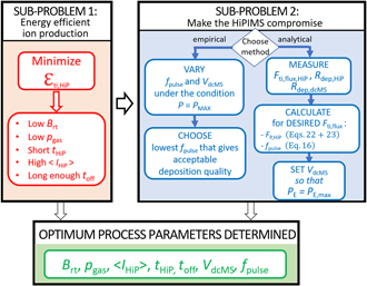
Figure 4. An illustration of HiPIMS discharge optimization in two steps: first, solving sub-problem 1, which minimizes the energy cost per ion placed on the substrate, and then solving sub-problem 2, making the HiPIMS compromise.
Download figure:
Standard image High-resolution imageFor the investigated Ti/Ar discharge we find that minimizing  requires: a low magnetic field strength, a low working gas pressure, a short HiPIMS pulse time, a high HiPIMS pulse discharge current, and a 'long enough' off-time after the HiPIMS pulses. By following these guidelines, we could reduce
  from about 25 000 eV in a poorly optimized HiPIMS discharge to about 9300 eV in an optimized discharge, with the possibility of reaching even lower values. Back-attraction of ionized sputtered species to the target is found to be the main reason for the difference in ion energy cost between the two discharges.
For the second sub-problem, called the HiPIMS compromise, the focus is shifted from the cathode target to the substrate. Here the task is to, for a given magnetron sputtering discharge in which  has been minimized, choose the lowest ionized flux fraction Fti,flux that gives the desired film properties for a specific application, as the deposition rate always decreases with increasing ionized flux fraction. We quantify the deposition rate loss by comparing the energy cost of depositing a neutral
  (1300 eV) versus an ion
  (9300 eV or more) onto the substrate. An unnecessarily high Fti,flux can therefore be seen as a waste of deposition rate which could have been higher. In practice, the second sub-problem can be expressed as finding the best combination of the two remaining process parameters: the HiPIMS pulse frequency fHiP and the dcMS voltage VdcMS. We propose two alternative methods to achieve this, which we call the empirical method and the analytical method. The empirical method is suitable for an operator who has one single specific application to optimize and wants a simple and goal-oriented method. The analytical method is more complicated but makes it possible to set the ionized flux fraction to a desired value, and to vary it in a predetermined way in time during the deposition process.
Acknowledgments
NB gratefully acknowledges the hospitality of CNRS and Université Paris-Sud, Orsay, where much of this study was conducted. NB also acknowledges the support of Svensk-Franska Stiftelsen. This work was partially supported by the Icelandic Research Fund (Grant No. 196141), the Swedish Research Council (Grant No. VR 2018-04139), the Swedish Government Strategic Research Area in Materials Science on Functional Materials at Linköping University (Faculty Grant SFO-Mat-LiU No. 2009-00971), and the Free State of Saxony and the European Regional Development Fund (Grant No. 100336119).
: Appendix.
We here give details for the influence 〈IHiP〉 → βt discussed in section 2.1.2. Figure 5 gives the relevant data, extracted from Butler [41]. It shows the effect of changing three parameters: the HiPIMS pulse length, the average pulse discharge current, and the working gas pressure. The diagram shows the fraction of the discharge voltage that drops over the IR f = VIR/VD versus the back-attraction probability of the ionized sputtered species.

Figure 5. Data extracted from Butler [41] which shows the fraction of the discharge voltage that is dropped over the IR f = VIR/VD versus the back-attraction probability βt of the ionized sputtered species. Four different series are given, where the working gas pressure and HiPIMS pulse length are varied. Each series contain results from three different average pulse discharge currents. The numbers in the boxes indicate the average discharge current 〈IHiP〉 during a HiPIMS pulse in units of A.
Download figure:
Standard image High-resolution image
As can be seen in figure 5, βt is influenced by the working gas pressure, the pulse length, and the average pulse discharge current, but we here only look for the effect of the discharge current. These four cases of interest are connected by lines. For all four combinations of working gas pressure and pulse length, βt is always lower for the high 〈IHiP〉 case (38 A) compared to the low 〈IHiP〉 case (9 A). There is consequently a clear trend such that a higher average discharge current during the pulse gives a lower ion back-attraction. This result is represented by a red (anti-correlation) arrow in figure 2.