Comparing equilibration schemes of high-molecular-weight polymer melts with topological indicators

Luca Tubiana; Hideki Kobayashi; Raffaello Potestio; Burkhard Dünweg; Kurt Kremer; Peter Virnau; Kostas Daoulas

doi:10.1088/1361-648X/abf20c

1. Introduction

Computer simulations of concentrated polymer solutions and melts based on microscopically-detailed models are an important numerical tool for tackling various questions in fundamental polymer physics [1, 2] and technological applications [3–8]. Frequently, however, these questions can be properly addressed only in a truly polymeric regime and require, therefore, simulations of high-molecular-weight (MW) polymers. Enabling equilibration of liquids comprising high-MW polymers at high concentrations, such as concentrated solutions and melts, is among the challenges of modern computational molecular physics.

Even though very efficient parallelized implementations are available [9–11], the generation of uncorrelated configurations with brute-force molecular dynamics (MD) requires considerable computational efforts. The reason is the protracted polymer dynamics in the entangled regime, where, for example, the reptation time (the largest of the characteristic relaxation times of molecular conformations) scales as τ_rep ∼ N³ [2, 12], where N stands for the polymerization degree. Even in the case of generic microscopic bead-spring models [13], the slow dynamics of long polymers limits the applicability of MD simulations to chains with about a thousand beads.

To circumvent the large relaxation times of brute-force MD, several alternative equilibration procedures have emerged in recent years. For example, advanced connectivity altering Monte Carlo (MC) algorithms [14, 15] can handle long polymers described either by generic [16, 17] or chemistry-specific [14, 15] models. Auhl et al [16] have proposed the so-called configuration assembly method, where the basic idea is to start with an ensemble of phantom chains and slowly introduce excluded volume interactions. Recently, powerful hierarchical backmapping strategies have been developed [18–25] enabling the equilibration of melts of unprecedented size, e.g. thousands of chains with length equivalent to several tens of entanglement lengths [18]. Some of these divide-and-conquer methods are based [18–22] on the idea of successively refining a blob-based model [26]. In this approach, stepwise fine-graining of configurations, first equilibrated at the lowest resolution, is employed until reaching a blob-based representation where the level of detail is sufficiently high to allow for reinsertion of microscopic features.

Configuration assembly and hierarchical backmapping methods yield [18] consistent results in terms of standard quantifiers of liquid structure and polymer conformations. Structural comparison is typically performed on the level of intra- and intermolecular pair distribution functions, whereas the consistency of conformations is validated comparing internal distance plots. The latter quantify the mean square distance between intramolecular monomers in space as a function of the difference of their ranking numbers along the chain backbone, i.e., the chemical distance. The deviations between internal distance plots in melts equilibrated by the two methods amount to a few percent [18, 19], at most. For many polymer properties such deviations translate into negligibly small effects. For example, the entanglement length N_e scales in melts of flexible chains as N_e ∼ ρ₀ p³ [27, 28], where ρ₀ is the average density of monomers and p is the packing length, defined [27, 29] as $p=N/{\rho }_{0}{R}_{\mathrm{e}}^{2}$ . Here ${R}_{\mathrm{e}}^{2}$ stands for the mean square distance between the ends of the polymer. Hence, deviations on the order of 1% in the internal distance plot indicate that the corresponding variations in estimations of N_e will be (at most) comparable to 3%. At the same time, recent studies [30] have demonstrated that such small deviations in internal distance plots still can result in substantial differences in topological properties of polymers expressed through the behaviour of molecular knots.

Knots are self-entanglements of chains which appear naturally in long [31–33] or confined polymers [34], as well as in dense polymer solutions, and biological systems [35–40]. Different knots appear with different probabilities and geometrical properties depending on various features of the polymers in which they are tied. This fact opens the possibility to use their relative frequency -called knot spectrum- as a fingerprint of the properties of a polymeric system, a technique which has been experimentally and computationally used to characterize the arrangement of DNA inside bacteriophage capsids [41–44].

Motivated by the observations above, here we compare the behaviour of polymer knots in melts prepared through configuration assembly and hierarchical backmapping methods. Evidence that knots are a good gauge for the overall structure of polymers has already been provided in a number of previous studies [40, 45]. We find that the two sets of melts show consistent knotting behaviour, providing additional evidence that the two techniques deliver equally equilibrated melts.

In contrast to single polymers [39, 40, 46–53] surprisingly little is known about knots in multichain systems. Therefore, quantifying knotting properties in polymer melts is of significant interest on its own. So far, knotting probabilities in melts of hard sphere chains have been determined [54, 55] to depict connections between intra- and interchain entanglements. Reference [45] demonstrates that knots are much less prevalent in melts than expected from a corresponding random walk model, indicating that ideal chains do not capture this structural aspect correctly. Building upon this work, a recent study showed [30] that knots in melts are well-described by mesoscale models with soft potentials if the length scale which characterizes polymer stiffness, i.e. the Kuhn length, is substantially larger than the size of typical excluded volume interactions. Vice versa, soft models typically perform poorly for flexible chains [30].

In our study, the analysis of knotting properties of melts of long chains leads to several findings of fundamental interest. For example, we demonstrate that the occurrence of knots is consistent with theoretical predictions [31, 32, 56] that the probability of observing an unknot should decrease exponentially with chain length. So far, this prediction has been validated only for single-chain systems.

2. Model

The microscopic description of homopolymer melts is achieved on the level of a generic bead-spring model [57]. This standard model is well-suited for fundamental studies of dynamics and rheology of polymeric liquids, because it encapsulates essential features such as hard excluded volume interactions, strong covalent bonds, and high monomer density. Each homopolymer is represented by a chain of N monomers (beads) linked by finitely extensible nonlinear elastic (FENE) springs. The stiffness (persistence length) of the chain is controlled by assigning to the angle θ formed by two sequential FENE bonds an angular potential U(θ) = κ_θ(1 − cos(θ)). Here κ_θ is a positive constant. Non-bonded interactions between monomers are captured through a Weeks–Chandler–Andersen (WCA) potential, U_WCA (r). The parameters of the FENE and WCA interactions are set to their standard values [18, 57, 58]. The configurations of the melts are cubic samples with volume V. They contain n chains such that the average density of the monomers is ρ₀ ≃ 0.85. Table 1 summarizes the number of chains, the polymerization degree, and stiffness parameters of the homopolymer melts that are analysed in this study with respect to knot properties.

Table 1. Number of chains n_α, polymerization degree N, and stiffness parameter κ_θ for the homopolymer melts considered in this study. For the number of chains, the subscript α = CA or BP denotes the equilibration method, i.e. configuration assembly or backmapping, respectively. The number of independent samples generated in each case via the two algorithms is also indicated.

N	n_CA	n_BP	κ_θ	Configuration-assembly	Backmapping
500	1000	4000	0.0	5	6
1000	1000	2000	0.0	5	3
1000	1000	2000	0.75	3	6
1000	1000	2000	1.0	4	7
2000	1000	1000	0.0	5	5

3. Equilibration algorithms

In this work, we add a new perspective to the analysis of polymer conformations in homopolymer melts equilibrated with an existing (i) configuration assembly [16, 58] and (ii) hierarchical backmapping [18–22] algorithm. Nevertheless, to facilitate the presentation of our topological analysis, it is useful to recapitulate the main features of these algorithms.

3.1. Configuration assembly algorithm

The configuration assembly method [16, 58] is by now an established stand-alone method for equilibrating polymer melts with moderate chain lengths. In the framework of the more powerful but less traditional hierarchical backmapping strategies, configuration assembly provides reference data for (i) parameterizing the blob-based model and (ii) validating equilibration of large samples obtained via hierarchical backmapping.

All reference data involved in our study were obtained [58] using a configuration assembly procedure [16] that first generates chains with conformations drawn from a distribution expected for the studied melt. Subsequently, these chains are treated as rigid bodies and arranged under relaxed constraints of excluded volume. An ensemble of randomly placed molecules is equivalent to an ideal gas of polymer chains so it exhibits density fluctuations that are unrealistically high for an interacting polymer liquid. To avoid significant conformational distortions during reinsertion of excluded volume on the monomer scale, these fluctuations are quenched through an MC procedure. After the density fluctuations are quenched, the configurations are subjected to a slow 'push-off' where the non-bonded WCA potentials are 'force-capped' according to the rule:

$\begin{align}\hfill & {U}_{\text{WCA}}^{\text{fc}}\left(r\right)=\begin{cases}\left(r-{r}_{\mathrm{c}}\left(\tau \right)\right){U}_{\text{WCA}}^{\prime }\left({r}_{\mathrm{c}}\left(\tau \right)\right)+{U}_{\text{WCA}}\left({r}_{\mathrm{c}}\left(\tau \right)\right),\quad r{\leqslant}{r}_{\mathrm{c}}\left(\tau \right)\quad \hfill \\ {U}_{\text{WCA}}\left(r\right),\quad \text{otherwise}\quad \hfill \end{cases}.\hfill \end{align} \tag{ 1 }$

Here r_c(τ) is the force-capping radius at step τ of the push-off and the original interactions are recovered when r_c(τ) → 0. During the push-off, realized using MD, the strength of the force capping is continuously adjusted through a feedback loop [58] to minimize the deviation of molecular conformations from those in the equilibrium melt. Because we will consider the behaviour of knots during such feedback loops, we provide a few more details on this procedure.

Specifically, after a few MD steps are performed with fixed r_c(τ), the conformational distortions are quantified using the descriptor:

$\begin{equation}I={\int }_{{n}_{\mathrm{1}}}^{{n}_{\mathrm{2}}}\left[\frac{\langle {R}^{2}\left(l\right)\rangle }{l}-\frac{\langle {R}_{\text{ref}}^{2}\left(l\right)\rangle }{l}\right]\mathrm{d}l.\end{equation} \tag{ 2 }$

Here ⟨R²(l)⟩ is the mean square distance between two monomers that belong to the same chain and have a chemical distance of l monomers. ⟨R²(l)⟩ is calculated in the melt configurations obtained with the given r_c(τ). Conversely, $\langle {R}_{\text{ref}}^{2}\left(l\right)\rangle$ is the reference value of mean square distance in melts of short chains that have been equilibrated with brute-force MD, i.e. without any conformational assembly. For bead-spring models, the integration boundaries in equation (2) are typically on the order of [58] n₁ = 20 and n₂ = 50–100. After a few MD steps, r_c is increased or decreased, depending on whether I is positive or negative.

3.2. Hierarchical backmapping algorithm

The hierarchical backmapping algorithm employs a hierarchy of blob-based models with different resolution, as illustrated in figure 1. The homopolymers described by the microscopic model are coarse-grained [26] into chains comprising soft spheres (blobs). For this purpose, each homopolymer is 'divided' into sub-chains consisting of N_b beads. Each sub-chain is replaced by a sphere; the coordinates of the centre of the sphere match the position of the centre-of-mass (COM) of the underlying subchain. In this way, each homopolymer is mapped on a CG chain with N_CG = N/N_b blobs. The resolution of the model at each level of the hierarchy is determined by the amount of microscopic monomers N_b underlying each sphere.

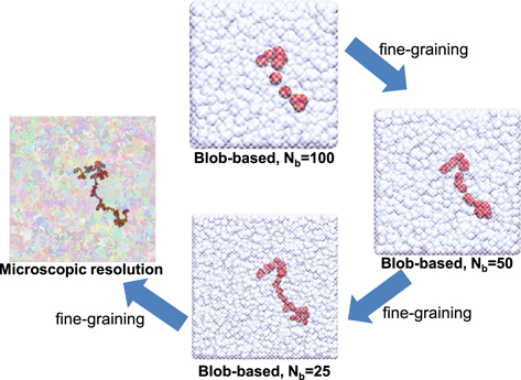
Figure 1. Refer to the following caption and surrounding text. — **Figure 1.** Schematic illustration of the hierarchical backmapping strategy [18]. The homopolymer melt is initially equilibrated using a blob-based model where each blob represents a large number of N_b monomers (in this sketch N_b = 100). After equilibration, the melt is sequentially fine-grained by reinserting the degrees of freedom of finer blob-based models (here N_b = 50 and 25). The microscopic features are reinserted once the blobs become sufficiently small. Colours are randomly chosen in the last microscopically-resolved configuration to improve the visibility of different chains.
Download figure:
Standard image High-resolution image

The description of the bonded and non-bonded interactions between the blobs has been elaborated in detail in several earlier studies [18–20, 22, 26, 59]. We briefly summarize that N_CG blobs are connected into a chain by simple harmonic bond and angular potentials, motivated by universal properties of random walks [60]. In the first implementations of hierarchical backmapping [18–20], non-bonded interactions between blobs were described by Gaussian potentials with fluctuating variance $\bar{\sigma }$ . These fluctuations of $\bar{\sigma }$ represent [26] fluctuations of the instantaneous radius of gyration of microscopic subchains underlying the interacting blobs. Here, we employ a later version [22] of the blob-based model where the non-bonded potentials are extracted from integral equation (IE) theory [61, 62]. Compared to empirical Gaussian potentials, non-bonded interactions defined via IE theory allow for a more straightforward parameterization [61, 62] for each choice of N_b.

Once the blob-based models are defined, large samples of melts with long polymer chains are efficiently equilibrated using the model with the crudest resolution (in figure 1 this crude model corresponds to N_b = 100). For this initial equilibration, we subjected the crude model to MD runs [22] lasting about nine Rouse times of the blob-based chains (chain dynamics is Rouse-like because of soft non-bonded interactions). Such long runs ensure proper sampling of topological properties of blob-based chains. After equilibration, the melt configuration is subjected to sequential fine-graining which descends the levels of the hierarchy by doubling the resolution at each step [18]. At each fine-graining step, each blob in the melt is replaced by a pair of two smaller ones, so that the COM of this 'dumbbell' coincides with the COM of the substituted blob. After this substitution, the local polymer conformations and the liquid structure must be re-equilibrated. However, this procedure involves only relaxation on local scales, whose associated times are short.

The configurations of the coarse-grained melt obtained from the last fine-graining step in the hierarchy of blob-based models (in figure 1 the finest blob-based model corresponds to N_b = 25) are used to recover the microscopic description. Initially, each soft-sphere polymer is replaced by a microscopic chain where the molecular architecture is controlled by the full set of the microscopic bonded potentials (cf section 2). However, all non-bonded interactions, except those between intramolecular nearest neighbours, are deactivated at this stage. The conformations of the soft-sphere polymer and its replacing microscopic chain must be consistent with each other. Therefore (i) the positions of the COM of each microscopic subchain must coincide with the COM of the corresponding blob and (ii) the radius of gyration (squared) of each microscopic subchain must equal the radius (squared) of the corresponding blob. Both requirements are achieved by 'driving' the substituting microscopic polymer into the substituted soft-sphere chain with the help of two pseudo-potentials [18]. This step is very fast, because the system at this stage presents an ensemble of non-interacting chains in external fields (the pseudo-potentials).

Finally, the microscopically resolved configuration is subjected to the push-off procedure [16, 58], already described in the context of the configuration assembly algorithm. After the push-off, the sample is locally re-equilibrated. The push-off and re-equilibration require only short MD runs, provided that the number of microscopic monomers underlying the blobs in the melt, where the microscopic details are reinserted, is sufficiently small. In particular, N_b must be smaller than the microscopic entanglement length N_e, i.e. N_b < N_e. In this case, the time scale required for re-equilibration is comparable to the Rouse time, τ_e, of a subchain with N_e monomers [12].

In the first implementations [18, 19] of hierarchical backmapping, the various stages were realized through a mixture of MC [59] and MD algorithms. Currently, the entire procedure of hierarchical backmapping is available [22] on the efficient ESPResSo++ platform [11] and is realized using only MD.

4. Knot analysis

Mathematically, knots are topological objects defined on closed, non-intersecting curves. Two closed curves contain the same knot if one of them can be transformed into the other without cutting it temporarily open. When no such transformation is possible, the two curves contain different knots. Conventionally, knots are pictured projected onto a plane, and tabulated according to the minimum crossing number, n_c, with which they can be represented, see e.g. reference [2]. Thus, the unknotted curve is called 0₁ as it can be pictured as circle; the simplest knot, the trefoil, is called 3₁ as it can not be projected with less than three crossings. The subscript in this notation is just a label to distinguish prime knots which have the same n_c, as e.g. 5₁ and 5₂ in figure 2. Prime knots can be joined together to form composite knots. For example, the knot with the label 3₁#3₁ in figure 2 is obtained by 'gluing' together two 3₁ knots. One can think of composite knots as being obtained by tying several prime knots onto a string, before joining its ends to circularize it.

Figure 2. Refer to the following caption and surrounding text. — **Figure 2.** (a)The minimal representation of knots up to six crossings, together with their standard notation based on the minimal number of crossings. Note that removing a single crossing from all these knots, except 5₁, is enough to unknot them. (b) Minimal representation of two composite knots, 3₁#3₁ and 3₁#4₁.
Download figure:
Standard image High-resolution image

Projections of a knot having n_c crossings are called minimal projections. The minimum crossing number n_c is the simplest example of topological invariant: a function of the curve whose value depends only on the type of knot tied on it, and not on its particular geometrical conformation. n_c is a weak topological invariant, as there are several knots for which it has the same value.

Knot theory provides us with powerful invariants to distinguish different knots. These are often based on polynomials built by assigning different mathematical forms to different crossings in the projection of a knot. In this study, we adopt two invariants. The first is the Alexander determinant; a fast polynomial-based invariant which is able to distinguish knots with up to seven crossings [33]. The second is given by the Dowker–Thistlethwaite code: tabulated sequences of integers which can be computed from minimal knot projections and identify prime knots up to 16 crossings [63, 64]. We refer the interested reader to the introductory book by Adams [64] and to more technical reviews written for physicists [33, 34] and biophysicists [36].

While mathematically knots are defined only on closed curves, physical knots appear most frequently on open chains. Furthermore, their tightness or looseness affects both the knot's and the polymer's mechanical and rheological properties. For example, tight knots have been shown to reduce polymers' tensile strength [65]; knotted DNA filaments are more compact than their unknotted counterparts, and take a long time to unravel [66]. Understanding knots' emergence and behaviour is particularly relevant for emerging technologies such as DNA sequencing. Both experimental and computational studies have shown that knots' behaviour, including their average size, diffusion constant and untying time, depend both on the polymer and on the knot properties, see e.g. references [67–71]. Furthermore, when more than one prime knot are present on a polymer, they tend to interact, and have a high probability of becoming intertwined [52, 72, 73].

To characterize physical knots' properties, one has to locate and classify them on open chains. Those are notoriously challenging tasks, since all the tools provided by knot theory are defined only for closed curves. To apply them to physical knots it is thus necessary to first circularize the open chains. In our analyses, we adopted the minimally interfering closure [74] to join the ends of open chains, and specifically its implementation in Kymoknot (www.kymoknot.sissa.it, source available from https://github.com/luca-tubiana/KymoKnot), a webserver and software package to localize knots on linear or circular chains [75]. The minimally interfering closure works by computing the convex hull of the (portion of) chain to be circularized, the distance between the two ends of the chain, and the distance between each of those and the surface of the convex hull. If the two ends are closer to the surface of the convex hull than they are to one another, each of them is connected to its closer point on the hull and the chain is circularized outside the convex hull. Otherwise, the ends are simply bridged [74]. This effectively minimizes the length of the fictitious circularizing curve within the convex hull.

Our knot analysis pipeline proceeds as follows. First, we circularize each chain in the melt independently of the others, and evaluate its topological status (knot) using both the Alexander determinants implemented in Kymoknot, and the Dowker codes implemented in KNOTFIND [63]. This first step allows us to construct the knot spectra of melts by constructing the histograms of the knot frequencies across different configurations of the same melt (see table 1).

Having identified the knotted chains, we proceed to localize their knotted portion using the stand-alone version of Kymoknot. Specifically, for each chain we perform a 'bottom-up' search which identifies the smallest region of the chain having the same Alexander determinants in t = −1 and t = −2 as the whole chain (see e.g. references [33, 75] for details). This means that in the case of a composite knot, the algorithm returns the shortest portion of the chain containing all the prime components of the knot. To speed up this step, we perform a mild smoothing of the chains by removing subsequent beads whose removal does not result in a crossing of the chain with itself. To maintain a good precision on the identified knotted region, we do not remove more than five consecutive beads. This smoothing procedure is described in detail in reference [75].

To avoid spurious differences in the analysis performed on samples obtained from the configuration assembly algorithm and those obtained from the backmapping algorithm, the whole pipeline (chain circularization, KNOTFIND-based knot identification, Kymoknot-based knot localization, data pooling) is completely scripted and executed automatically in the same way for both sets of melt configurations.

5. Results

In this section we present and discuss results obtained from our analysis. We start by describing some characteristic structural and conformational features of polymer chains in melts prepared with the two different algorithms and perform a comparison of the two; subsequently, we focus on topological properties, which constitute a particularly stringent fingerprint of melt equilibration.

5.1. Comparison of structural and conformational properties

Previous studies [18–22] have demonstrated that melts equilibrated with configuration assembly and hierarchical backmapping are consistent with each other in terms of standard conformational and structural properties. As an illustration, in the remainder of this subsection, we consider a representative system: a melt of chains with length N = 1000 beads and strength of the angular potential κ_θ = 1. Focussing on this particular case serves a twofold purpose: on the one hand, we illustrate the agreement between configuration assembly and backmapping; on the other hand, we introduce the typical quantitative descriptors employed to perform the comparison and showcase their usage.

We start by verifying the agreement of the liquid structure in the two approaches through a comparison of the monomer–monomer pair-distribution functions g(r). In figure 3(a) we report data obtained from melts generated with configuration assembly (blue line) and hierarchical backmapping (red symbols): the curves are practically indistinguishable from each other, as the data points overlap well within the point size. An even stronger evidence on the consistency of the liquid structure in the two approaches is provided in figure 3(b), which presents the intermolecular part of the pair-distribution function, g_inter(r). The almost perfect agreement of the plots confirms that the packing of the liquid on larger scales, that is the correlation hole between polymer chains, is also reproduced.

Figure 3. Refer to the following caption and surrounding text. — **Figure 3.** (a) Monomer–monomer pair distribution function g(r) in melts equilibrated using configuration assembly (blue line) and hierarchical backmapping (red symbols). The length of the chains and the strength of angular potential are N = 1000 and κ_θ = 1, respectively. (b) Intermolecular monomer–monomer pair distribution function g_inter(r) for the same systems as in panel (a).
Download figure:
Standard image High-resolution image

Subsequently, we turn to larger-scale intra-chain properties, that is, the internal distance plot. This quantity corresponds to the ratio C(l) ≡ ⟨R²(l)⟩/l (the definitions of ⟨R²(l)⟩ and l are the same as in section 3.1). Figure 4(a) presents the internal distance plots obtained with the two methods. We quantify their consistency by computing the relative deviation between the two datasets defined as:

$\begin{equation}\delta \left(l\right)=\frac{C\left(l\right)-{C}_{0}\left(l\right)}{{C}_{0}\left(l\right)},\end{equation} \tag{ 3 }$

where C(l) and C₀(l) indicate the internal distance plot calculated in backmapped and assembled melts, respectively. The data on δ(l) are presented in figure 4(b) and demonstrate that the relative deviation of the internal distance plots between the two methods does not exceed 1.5%.

Figure 4. Refer to the following caption and surrounding text. — **Figure 4.** (a) Internal distance plots ⟨R²(l)⟩/l calculated for melts equilibrated using configuration assembly (blue squares) and hierarchical backmapping (red circles). The length of the chains and the strength of the angular potential are N = 1000 and κ_θ = 1, respectively. Error bars, when not visible, are smaller than the symbols. (b) Relative deviations δ(l) of internal distance plots reported in panel (a) (cf equation (3)). The error bars of δ(l) are represented by the shaded area. Both in panel (a) and (b) error bars correspond to 1.96σ, i.e. a 95% confidence interval.
Download figure:
Standard image High-resolution image

5.2. Comparison of knotting behaviour

We now turn our attention to the comparison of topological properties of melts generated using configuration assembly and hierarchical backmapping, cf table 1. An example conformation of the simplest knot, the 3₁ is reported in figure 5. Our analysis considers the main topological characteristics that are commonly investigated in single-chain studies, namely the unknotting probability, i.e. the probability that a chain contains no knots, P_un, the knotting probabilities of the most common knots (knot spectra), and the linear size of the knotted portion, the knot length l_knot. The investigation is carried out for melts of flexible chains of length N = 500, 1000, and 2000; for the case N = 1000 three different values of bending stiffness are explored, that is, κ_θ = 0.0, 0.75, 1.0.

Figure 5. Refer to the following caption and surrounding text. — **Figure 5.** A tight trefoil knot located far from the ends of the chain; the knot contour is highlighted in red. This snapshot corresponds to a configuration generated with the hierarchical backmapping strategy; similar tight knots have been observed in chains generated with the configuration assembly method.
Download figure:
Standard image High-resolution image

Before presenting our results on knotting properties, we discuss some details related to the statistical analysis of related data. Although both the melt equilibration and the knot analysis strategies are state-of-the-art, a proper quantification of some properties, e.g. the knot length distribution, requires large amounts of knotted chains, which are not always available to us. In fact, while our samples contain thousands of chains, only a fraction of them are knotted; in table 2 we report the total number of knotted chains n_knotted that have been considered for each system. In the following, if not otherwise stated, error bars are set to 95% confidence intervals. These correspond to 1.96σ, with σ the standard deviation of the mean of the observable. For the unknotting probabilities, the standard deviation has been computed based on the binomial statistics for Bernoulli trials: $\sigma =\sqrt{{P}_{\text{un}}\left(1-{P}_{\text{un}}\right)/n}$ , where P_un is the unknotting probability and n the total number of chains considered. For all studied melts P_un and n are listed in table 2. The same strategy has been used to evaluate the confidence level of the probabilities of specific knots. For the average knot lengths, σ has been calculated directly as the standard deviation of the sample of average values obtained from each melt realization, cfr. table 1.

Table 2. Knot statistics for the various melts considered in this study. For each pair of parameters N and κ_θ we report, for both equilibration strategies, the total number of chains considered, n, the total number of knotted chains n_knotted, the unknotting probability, P_un, and the average knot length ⟨l_knot⟩. Errors represent 95% confidence intervals.

Melt properties
N	κ_θ	Method	n	n_knotted	P_un	⟨l_knot⟩
500	0.00	Backmapping	24 000	929	0.961 ± 0.002	160 ± 7
500	0.00		Conf. assembly	5000	208	0.958 ± 0.006	172 ± 14
1000	0.00	Backmapping	6000	698	0.884 ± 0.008	247 ± 15
1000	0.00		Conf. assembly	5000	553	0.890 ± 0.009	257 ± 17
1000	0.75	Backmapping	12 000	1998	0.834 ± 0.007	233 ± 9
1000	0.75		Conf. assembly	3000	492	0.836 ± 0.013	245 ± 17
1000	1.00	Backmapping	14 000	2558	0.817 ± 0.006	213 ± 7
1000	1.00		Conf. assembly	4000	777	0.806 ± 0.012	231 ± 14
2000	0.00	Backmapping	5000	1251	0.750 ± 0.012	378 ± 21
2000	0.00		Conf. assembly	5000	1274	0.746 ± 0.012	403 ± 21

Figure 6(a) shows the unknotting probability in a melt as a function of chain length N. These data confirm, in the case of polymer melts, a hypothesis formulated in the early 1960s, the so-called Frisch–Wassermann–Delbrück [76,77] conjecture, which essentially states that the equilibrium conformation of any sufficiently long polymer chain will contain one or more knots. Indeed, this conjecture was shown to hold for many different polymer models in simulations (e.g. in [56]) and was even proven mathematically in 1988 for self-avoiding polygons on a simple cubic lattice [31,32]. In the latter work, it was also shown that, for long enough chains, the unknotting probability must decay exponentially:

$\begin{equation}{P}_{\text{un}}\propto \mathrm{exp}\left(-N/{N}_{0}\right),\end{equation} \tag{ 4 }$

with a characteristic size N₀ depending on the physical properties of the polymer, on its degree of confinement, and on the density of the solution or melt [33, 34, 78, 79]. As demonstrated in figure 6(a) and in table 2, equation (4) describes the unknotting probability of flexible open polymers in a melt equilibrated with the backmapping and the configuration assembly methods equally well, and the results obtained in the two cases are in excellent agreement with each other. The unknotting lengths are compatible within the standard error of the fit: N₀ = 6030 ± 48 for backmapping and N₀ = 6060 ± 300 for configuration assembly. Furthermore, the probabilities of the two most common knots, 3₁ and 4₁, agree throughout the investigated range of chain lengths within a 95% confidence interval, see figure 6(b).

Figure 6. Refer to the following caption and surrounding text. — **Figure 6.** (a) Unknotting probability P_un as a function of polymer contour length N (logarithmic scale) for melts obtained from configuration assembly (blue) and hierarchical backmapping (red). (b) Probabilities of observing the two most common knots, 3₁ and 4₁. Error bars represent 95% confidence intervals.
Download figure:
Standard image High-resolution image

The consistency between the two methods remains excellent when we fix the chain length, N = 1000 and consider different values of bending stiffness, as can be seen from the results reported in figure 7. We notice here that the unknotting probability decreases with increasing chain rigidity, that is, stiffer chains display stronger propensity to form knots, as shown by the histograms in panel (b). This result, while counter-intuitive at first sight, is in line with what has been observed in computer simulations of flexible and semiflexible single chains, both for lattice and off-lattice polymers [80–84]. These works have highlighted the competing role of energy and entropy in knot formation: while a knot restricts the accessible conformational space of a chain, its presence straightens it locally, thus relaxing the average bending energy. The competition of these two effects leads to a non-monotonic behaviour of the knotting probability as a function of the chain stiffness: for very small values of the persistence length the knot formation is entropically unfavourable; a large rigidity disfavours knots as it pushes the system towards extended, ideally circular conformations; in between there is an 'optimum' stiffness for which the two effects coherently favour the formation of self-entanglement, thereby increasing the knotting probability. Most remarkably, although our chains are still too flexible to observe the non-monotonic behaviour, our results suggest that this effect persists also in dense polymer melts.

Figure 7. Refer to the following caption and surrounding text. — **Figure 7.** (a) Unknotting probability as a function of chain stiffness κ_θ computed for chains in melts equilibrated with configuration assembly (blue squares) and backmapping (red circles) methods. (b) Knotting probability for 3₁ and 4₁ knots as a function of polymer stiffness for melts of chains with length N = 1000. Errors have been computed as in figure 6.
Download figure:
Standard image High-resolution image

Finally, we turn our attention to the geometrical properties of the knots themselves, namely the number of beads of the polymer that actually constitute the knotted portion, the so-called 'knot length', l_knot. We notice here that this quantity is well-defined for prime knots, while our sample can include composite knots as well. Nonetheless, in all our melts the latter appear with a frequency lower than 0.4% and thus do not affect the results. The agreement between configuration assembly and hierarchical backmapping can be appreciated by comparing the distributions of knot lengths obtained by the two strategies. These are reported using boxplots in figure 8. Specifically, figure 8(a) shows the l_knot distributions for flexible chains of different length, while figure 8(b) those for different values of κ_θ. Boxplots effectively capture the basic properties of a distribution: the boxes correspond to the first quartiles below, Q1, and above, Q3, the median of the distribution, and thus capture 50% of the observations. The median value is shown with a line and the mean value with a square. Finally, the whiskers report the outliers. In our case, they extend from the median to the lowest and highest outlier within 1.5IQR, with IQR = Q3 − Q1. As l_knot distributions are fat-tailed, the upper whiskers in figure 8 correspond effectively to the median of l_knot plus 1.5IQR; further outliers are ignored for clarity.

Figure 8. Refer to the following caption and surrounding text. — **Figure 8.** Box plots for knot length distributions as a function of chain length (a) and chain stiffness (b). As can be verified from table 2, the discrepancies between the boxes and whiskers for the two methods at κ_θ = 0.75 and κ_θ = 1.0 correlate with lower numbers of samples obtained from configuration assembly.
Download figure:
Standard image High-resolution image

In figure 8(a) the boxes are almost completely overlapping, while the difference in the whiskers' lengths can be ascribed to limited statistics, as observed in table 2. This is true, in fact, for most systems. A similar level of agreement is observed for the knot lengths obtained by fixing the degree of polymerization to N = 1000 and varying the stiffness of the chains, κ_θ, see figure 8(b). The agreement between the two methods is particularly evident for the system for which we have the largest amount of knotted configurations (in both cases), i.e. N = 1000, κ_θ = 1.0, reported in figure 9(a).

Figure 9. Refer to the following caption and surrounding text. — **Figure 9.** (a) Knot length histograms obtained for the melt N = 1000, κ_θ = 1.0 equilibrated using configuration assembly (blue line) and backmapping (red line). For this system we have 777 and 2558 knotted chains in melts generated with configuration assembly and hierarchical backmapping, respectively. (b) Knot length histograms for melt of flexible polymers of different lengths obtained through the backmapping equilibration strategy.
Download figure:
Standard image High-resolution image

The behaviour of the average knot length, ⟨l_knot⟩, has been studied extensively in the case of single chains in solution: one of the main results of these investigations is that knots are weakly localized [50, 85]; quantitatively, this means that their average length grows as a power law of the chain length, l_knot ∝ N^α, with 0 < α < 1, for both flexible and semiflexible polymers. The average knot lengths for all systems are reported in table 2 and show good agreement between configuration assembly and hierarchical backmapping. Interestingly, a decrease of ⟨l_knot(κ_θ)⟩ is observed for chains of increasing stiffness, compatibly with computational studies of semiflexible polymers in solution [81]. Furthermore, it is clear from the values of ⟨l_knot⟩ reported in table 2 that the knots are weakly localized in our melts, as observed by [86], as ⟨l_knot⟩/N decreases with N. Lastly, we notice that, although the differences between ⟨l_knot⟩ in melts prepared with the two methods are within the 1.96σ error bars, the trends in table 2 and figure 8 suggest that ⟨l_knot⟩ in backmapped melts is slightly smaller than in those prepared using configuration assembly. Observing slightly more compact knots in backmapped melts is consistent with the comparison of internal distance plots in figure 4. There, on intermediate scales, 10 ⩽ l ⩽ 100, chains in backmapped melts are effectively 'stiffer' than their counterparts in assembled melts. Such marginal differences might stem from technical details during the implementation of different algorithms, such as the speed with which excluded volume increases during the push-off stage. Exploring the effect of such technical details warrants a separate study.

The large number of knotted chains available for the melts equilibrated with backmapping, cfr. table 2, allows us to observe that the distribution of l_knot changes with increasing chain length (figure 9). As observed in previous computational studies on single knotted polymer chains, the most probable knot length is independent of the chain length N, while the average knot length grows with N due to the fact that the distributions are fat-tailed [72, 87] with their tails growing with the size of the polymer. This behaviour reflects the fact that the maximum knot length corresponds to the polymerization degree of the polymer, and that the number of ways in which a knot of size l_knot can be placed on a chain of size N is given by a combinatorial function, which decreases when l_knot increases.

Our consideration of knotting properties raises one important question. Blob-based models describe polymer conformations only down to length scales as small as the blob size. The reinsertion of microscopic beads bridges the gap between the resolution of the last blob-based model of the hierarchy and the microscopic description. In the beginning of the reinsertion, subchains with lengths comparable to N_b underlying the last blob-based model (in figure 1 this length is N_b = 25) are essentially ideal chains (cf section 3.2) and have [45] significantly more knots than non-ideal subchains in melts. Because the MD-based push-off realizes local dynamics, these spurious knots could, in principle, become 'locked' during the growth of excluded volume and lead to melts with unrelaxed topology.

Therefore, in figure 10 we present the evolution of P_un during the push off for a melt with κ_θ = 1 and N = 2000 (red line). The evolution of r_c controlling the excluded volume is reported on the same plot (grey line, with values on the right y-axis). The data for P_un confirm our expectations: the push-off starts from an ensemble of chains with significant number of knots. However, the number of knots decreases rapidly before the excluded volume recovers full strength. In other words, the insertion of the bead–bead potential only slowly introduces topological constraints on conformational rearrangements. Similar behaviour of knots during push-off has been observed in an earlier study [45]. Whereas the stage of push-off is present in both configuration assembly and hierarchical backmapping methodologies (cf sections 3.1 and 3.2), it starts in these two cases from qualitatively different initial configurations. Hence, the convergence of configuration assembly and hierarchical backmapping to melts with consistent knotting properties supports that the topology of chains is equilibrated in both cases.

Figure 10. Refer to the following caption and surrounding text. — **Figure 10.** The unknotting probability, P_un as a function of push-off time τ_LJ, measured in Lennard–Jones (LJ) units of time, is reported in red and on the left axis. The parameter controlling the excluded volume, r_c(τ_LJ) is reported in grey and on the right axis. The full strength of excluded volume, i.e. r_c = 0, is recovered at τ_LJ = 650.
Download figure:
Standard image High-resolution image

6. Conclusions

Our work considered two state-of-the-art schemes that are currently available for the equilibration of large samples of high-MW polymer melts: the configuration assembly [16, 58] and the hierarchical backmapping method [18–22]. These methods have been validated in earlier studies through an extensive comparison of standard quantifiers of liquid structure and polymer conformations. Here, we added a new perspective by comparing intramolecular topological properties—polymer knots—in melts with the same architectural and volumetric properties prepared using the two methods independently. A broad range of knotting properties was quantified, including the probability of the unknotted state, the probability of observing the two most common knots (3₁ and 4₁), and geometrical features of knots. For all topological properties we observed very good agreement. This consistency across samples prepared with two different methods provides additional evidence that both of them indeed converge to equilibrated melts.

The mutual agreement of all investigated topological properties in melts prepared with the two strategies is a remarkable fact, because knots capture both local (geometric) and global (topological) properties of polymers. Furthermore, knots are fine indicators: changing a single crossing is enough to change their topological signature. As a consequence, it would not be possible to conjecture our results only by observing that both configuration assembly and hierarchical backmapping produce melts with comparable internal distances and structural correlation functions. Our result is particularly important for the relatively new, and less explored, hierarchical backmapping method which has opened the way for equilibrating melt samples of unprecedented size and length [18–22]. Our analysis gives additional trust to recent extensions of these methods to interfacial polymer systems, such as homopolymer films [88].

Apart from providing an additional validation of the hierarchical backmapping method, our study delivered results that are interesting for the general theory of molecular knots. The large polymerization degrees considered enabled us to demonstrate, for the first time, that the probability of obtaining an unknotted state in polymer melts decreases exponentially with chain length. This observation is consistent with earlier mathematical predictions [31, 32] and simulations of single polygons [33, 56].

By confirming that hierarchical backmapping procedures can equilibrate polymer melts even on the level of self-entanglements, our study opens new opportunities for exploring topological properties of multi-chain systems, inaccessible to earlier equilibration techniques.

Acknowledgment

We thank Guojie Zhang and Torsten Stuehn for their assistance in accessing and properly interpreting pre-existing data on configurations of equilibrated melts. We are grateful to the Deutsche Forschungsgemeinschaft (DFG, German Research Foundation) for funding this research: Project Number 233630050-TRR 146. We would also like to acknowledge the contribution of the COST Action EUTOPIA (CA17139). LT acknowledges support from the MIUR grant Rita Levi Montalcini. HK and BD acknowledge support from the European Union Horizon 2020 research and innovation program under the Grant Agreement No. 676531 (project ECAM). HK acknowledges support from the Leverhulme Trust through research project Grant Number RPG-2017-203.

Dates

Peer review information