

Abstract
Carbon monitoring is critical for the reporting and verification of carbon stocks and change. Remote sensing is a tool increasingly used to estimate the spatial heterogeneity, extent and change of carbon stocks within and across various systems. We designate the use of the term wet carbon system to the interconnected wetlands, ocean, river and streams, lakes and ponds, and permafrost, which are carbon-dense and vital conduits for carbon throughout the terrestrial and aquatic sections of the carbon cycle. We reviewed wet carbon monitoring studies that utilize earth observation to improve our knowledge of data gaps, methods, and future research recommendations. To achieve this, we conducted a systematic review collecting 1622 references and screening them with a combination of text matching and a panel of three experts. The search found 496 references, with an additional 78 references added by experts. Our study found considerable variability of the utilization of remote sensing and global wet carbon monitoring progress across the nine systems analyzed. The review highlighted that remote sensing is routinely used to globally map carbon in mangroves and oceans, whereas seagrass, terrestrial wetlands, tidal marshes, rivers, and permafrost would benefit from more accurate and comprehensive global maps of extent. We identified three critical gaps and twelve recommendations to continue progressing wet carbon systems and increase cross system scientific inquiry.
Export citation and abstract BibTeX RIS

Original content from this work may be used under the terms of the Creative Commons Attribution 4.0 license. Any further distribution of this work must maintain attribution to the author(s) and the title of the work, journal citation and DOI.
1. Introduction
The Paris Climate Agreement requires net neutral carbon emissions by reducing fossil fuel emissions and balancing sources and sinks by 2100 [1]. Monitoring, reporting, and verification (MRV) are foundational for tracking emission reductions from land-use change and carbon removal attributed to reforestation and afforestation [2, 3]. Oceans, coasts, and wetlands are essential components of the global carbon cycle and are considered critical to achieving emission reductions necessary for fulfilling a variety of Sustainable Development Goals (figure 1) [4–6]. Carbon monitoring of wetlands, water bodies, and oceans pose unique challenges because of their complex ecosystem structure, seasonality, and susceptibility to climate impacts such as sea-level rise, drought, and increased storms [7, 8].
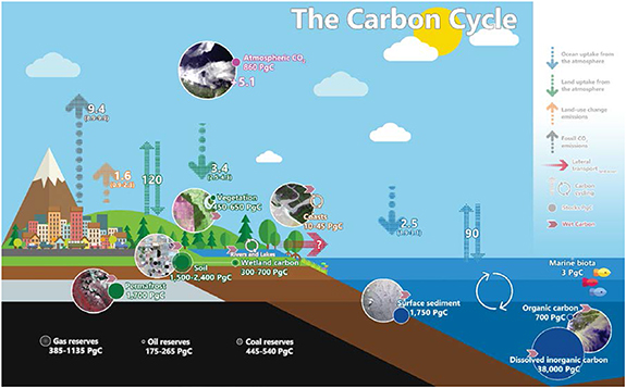
Figure 1. The global carbon cycle adapted from [9]. Wet carbon systems are highlighted with the interaction symbol from systems ecology [10]. Vegetation and soil are both denoted as wet carbon systems, but only a portion of these carbon stores are wet carbon. Images are Planetscope (permafrost, soil, vegetation, coasts), Sentinel-3 (atmospheric and organic carbon), and surface sediment camera system (photo credit Kevin Stokesbury). Wetland soil carbon value from Bridgham et al [11]. Photo credit: Kevin Stokesbury. Reproduced with permission.
Download figure:
Standard image High-resolution imageThis review focuses on the fluxes and stocks of carbon in wet carbon (WC) systems, a term used hereinafter to include all freshwater, saline, and brackish aquatic and wetland ecosystems, e.g. peatlands, mangroves, and oceans. This term is not a paradigm shift away from 'blue carbon' but a broader grouping of carbon cycle systems with shared data needs, restoration and preservation priority, and research direction. 'Blue carbon' is a term used to describe carbon-dense coastal wetland ecosystems and has aided significant research progress, with an expansive agenda for monitoring and applications [12]. However, focusing exclusively on 'blue carbon' ecosystems emphasizes ∼20% of global wetlands (1520–1620 Mha) and excludes terrestrial wetlands, permafrost, lakes, riverine, and marine systems [13, 14]. We primarily consider the oceans a WC system due to the interconnectedness between the oceans and other WC systems, i.e. the land–ocean aquatic continuum (figure 1) [15]. Here, we conducted a synthesis review of these interconnected systems to identify shared data needs, convergent research directions, and carbon monitoring goals.
Carbon monitoring research has rapidly expanded over the last 10–20 years due to international agreements targeted at reducing carbon emissions and establishing the need for accurate MRV of carbon. In 1997, the Kyoto Protocol prioritized the need for agricultural soils and forests to be managed as natural carbon sinks [16], followed by the development of Reduce Emissions from Deforestation and Forest forest Degradation (REDD) and REDD+ in 2009. The Paris Climate Agreement promotes wetland and coastal ecosystem management and provides a mechanism for developing and implementing their nationally determined contributions (NDCs) [16, 17]. The goal of carbon-neutral land-use change set forth as part of the Paris Climate Agreement has added additional exigency for developing MRV methods to inform carbon offsets and facilitate the inclusion of WC ecosystems within NDCs. To continue the further expansion of carbon offsets to WC systems requires high-quality remote sensing enabled MRV, a core goal of the NASA Carbon Monitoring System (CMS) Program [18].
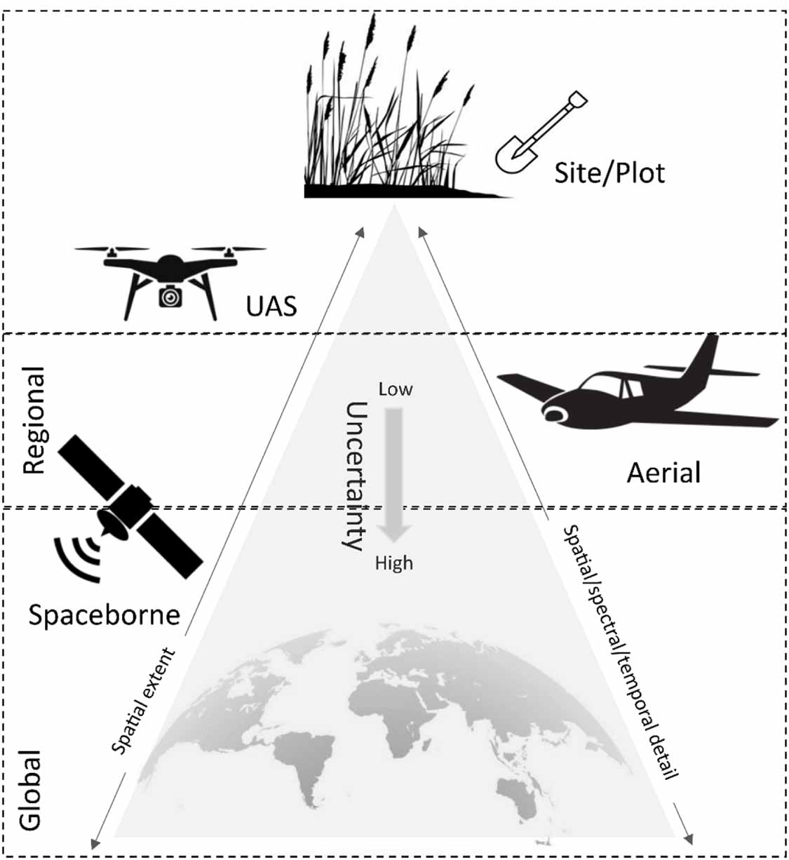
Remote sensing data provide spatial and temporal observations that can support carbon monitoring at local, regional, and global scales. WC monitoring of terrestrial and coastal wetlands are concerned with both aboveground and subsurface carbon as most of these systems' carbon stock is below the surface [19]. Tier 3 Intergovernmental Panel on Climate Change (IPCC) estimates require the inclusion of modeled, local processes that impact emissions and reduce uncertainty [20]. Therefore, spatially resolving subsurface carbon requires modeling of hydrological, biophysical, and topographic indicators [21]. At local scales, carbon MRV can be conducted exclusively with in situ data. However, WC monitoring at regional and global scales requires combinations of in situ measurements and remote sensing observables. Remote sensing introduces uncertainty but helps resolve spatial variability that in situ estimates cannot (figure 2). Enabling our end goal of global continuous monitoring of all WC systems and their interactions.
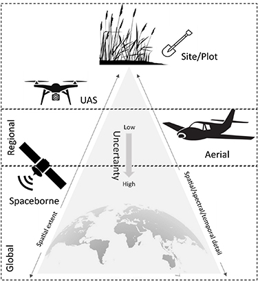
Figure 2. Terrestrial carbon monitoring extents, platforms in relation to uncertainty and remote sensing spatial, temporal, and spectral resolution domains.
Download figure:
Standard image High-resolution imageThe NASA CMS program seeks to prototype methods for MRV of the entire carbon cycle, and these WC systems represent an essential component with unique data needs and methodologies. As part of this review, we surveyed nine WC systems to determine earth observation-based WC monitoring status within each. The inclusion of more systems into global carbon budgets can reduce uncertainty, improve modeling outputs, and diversify climate mitigation solutions. WC monitoring is a relatively new field that we explore through a systematic review of the literature identifying gaps in our understanding, including location, ecosystem function, and methodological. We set forth the current state of carbon monitoring science within a subset of WC systems, including mangroves, peatlands and permafrost, tidal marsh and flats, terrestrial wetlands, oceans, coastal and continental shelf seas, lakes and ponds, rivers and streams, and submerged aquatic vegetation (SAV) (including seagrasses, kelp). We focus on natural WC systems due to their connections and shared data needs; it should be noted that anthropogenic WC systems, such as, rice paddies, are also important, but beyond the scope of our review. We discuss the current state of carbon monitoring data, stakeholder engagement, and provide recommendations to inform the future of WC monitoring, the NASA CMS program, and carbon accounting.
2. Systematic review
2.1. Methodology
The Web of Science was used to conduct this review with the inclusion of the CMS literature archive, and Google Scholar searches. Our search descriptions and strings can be found in supplemental table 1 (available online at stacks.iop.org/ERL/17/025009/mmedia). This example search string resulted in 466 references within the Web of Science and cumulatively all searches amounted to 1622 records. The system terms used included salt marsh, tidal marsh, mangroves, wetland, coral, seagrass, forested wetland, riparian, bog, peat, benthic, ocean, tidal flat, mudflat, marsh, bog, vernal pool, salt flat, submerged aquatic vegetation, beach, kelp, and playa. The Google Scholar results, and CMS program outputs were screened with an automated text selection algorithm, ensuring that all abstracts had a remote sensing and WC system term. The resulting studies were input into Cadima, a webtool for facilitating systematic reviews. All abstracts were screened by at least two reviewers to identify if they fulfilled three requirements.
- (a)The study used remote sensing data
- (b)The study reports carbon monitoring findings (land cover mapping or solely in situ finding were excluded)
- (c)The study at least partially focuses on a WC system
If all these questions were answered in the affirmative, we included that paper in the data extraction step of the literature review. If reviewers disagreed on an abstract's relevancy, a three-reviewer panel adjudicated its inclusion with most references being passed to the next step i.e. full review by an expert on that system. This process found 496 relevant references. Additional references were added based on expert knowledge resulting in a total of 574 (supplemental data 1). The references were divided into WC systems including mangroves (n = 79), tidal marsh and flats (n = 47), (SAV; n = 45), mineral wetlands (n = 55), peatlands (n = 129), permafrost (n = 80), lakes (n = 64), rivers (n = 33), oceans (n = 102), and ocean shelf (n = 30). References were allowed to have multiple system designations.
3. Results
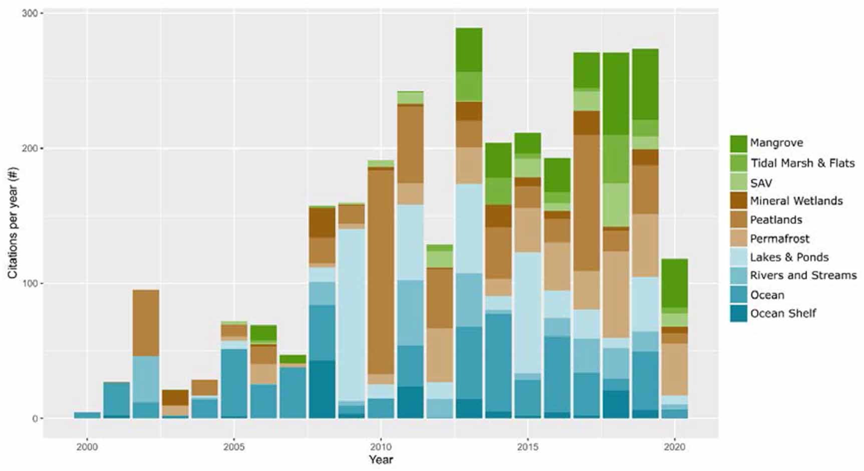
Since 2010, studies of WC monitoring with remote sensing have increased substantially (figure 3). The research growth tracks with major literature milestones, e.g. Nellemann et al [22], which first coined the term 'blue carbon,' and Page et al [23], which demonstrated the importance of tropical peatland carbon. Interest further developed with a call for the use of remote sensing to identify land-use change, priority areas for protection, and methods for measuring C stocks within sediments [24]. However, growth was not consistent between WC systems, with some having more research interest, including oceans, peatlands, and mangroves.

Figure 3. The results of the systematic review. References separated by year and WC system. We have separated peatlands and permafrost from terrestrial wetlands to demonstrate the disparity in research interest.
Download figure:
Standard image High-resolution imageDisparate levels of research interest across remote sensing monitoring of WC systems are evident in this result. In the past, 'blue carbon' research and media coverage were highly skewed towards coral [25]. Realignment of research interest, media attention, and funding is critical for understanding understudied WC systems and providing scientific justification and public support for WC mitigation. However, total yearly citations demonstrate that WC research utilization has remained relatively consistent since 2010 (figure 4) despite more studies. Many systems are still developing remote sensing methodologies to enable carbon monitoring (see sections 3.1.2, 3.1.3, 3.2.1 and 3.3.2). A shared language of carbon monitoring was evident across our WC systems. The use of earth observation to capture spatial heterogeneity is apparent in the two most common keywords, i.e. dynamics and variability. These keywords were identified in clusters across the literature and were areas of shared interest (figure 5). Thematic mapping of the literature revealed that climate change, dynamics, and carbon were the most fundamental research themes and that forested WC systems were prominent in multiple clusters. These two forest-related clusters correspond with peatlands and mangroves, two systems with considerable growth in research interest from 2000 to 2019 (figure 3). An emerging cluster associated with coastal remote sensing was evident, likely due to a recent focus on the data requirements for monitoring coastal systems. These keywords were apparent within our detailed reviews of WC systems and framed our discussion of the status of carbon monitoring.

Figure 4. Total average citations per year by publication year and WC system category.
Download figure:
Standard image High-resolution image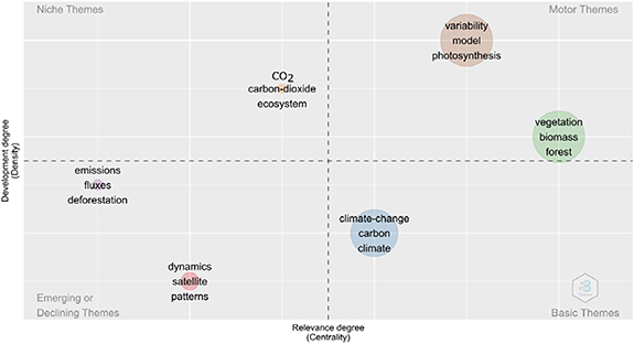
Figure 5. Thematic map created using keywords of WC research. We plotted relevance i.e. connection to the body of research on the x axis and development i.e. connections within a cluster on the y axis—each cluster's three most common keywords represent it. The Bibliometrix package in R 4.1.1 [26, 27].
Download figure:
Standard image High-resolution image
WC systems were separated into three categories for this review: coastal wetlands, inland wetlands, and ocean and shelves. Coastal wetlands included mangroves, SAV, and tidal marshes and flats. Inland wetlands comprised of mineral wetlands, peatlands and permafrost, whereas, inland waterbodies, lakes and ponds, and rivers and streams. Each of these system sections discusses the status of carbon monitoring within the system.
3.1. Coastal wetlands
Coastal wetlands are located along the terrestrial-aquatic interface and influenced by ocean and freshwater processes [28]. 'Blue carbon' ecosystems (seagrass, mangroves, tidal marshes and forests) comprise a portion of coastal wetlands. Coastal wetlands have consistently lost extent across the 19th and 20th century (−0.228% yr−1), slightly less than inland wetland loss (−0.391% yr−1) [29].
3.1.1. Mangroves
In total, we found 79 papers relevant to carbon monitoring with remote sensing in mangrove ecosystems. Mangroves have some of the highest carbon (C) density (401 ± 48 Mg C ha−1), with between 49%–98% of carbon stored in the soils [30]. Mangroves are a small fraction of global forest area (0.3%–0.5%) but a significant global C stock (5–10.4 PgC) [21, 31–36]. Recently, Global Mangrove Watch identified 137 600 km2 of mangrove extent in 2010 and has since measured change from 1996 to 2017 [35, 37]. These forests are under significant threat from anthropogenic activity and sea-level rise [38–40]. In general, mangroves are difficult to survey, but remote sensing has increased our capacity to monitor their extent, C stocks, and change. We have grouped our synthesis of the status of carbon monitoring in mangroves into three sections: (a) carbon monitoring status, (b) data and applications.
3.1.1.1. Carbon monitoring status
Not long ago, mangrove biomass and carbon estimates relied upon the extrapolation of field data, environmental conditions, and partial extent maps [e.g. 31, 41–45]. Giri et al [46] created the first global mangrove map using Landsat imagery. This map and other advances in remote sensing have enabled regional-to-global-scale analyses of mangrove carbon stocks and carbon stock change [21, 36, 38, 40, 47–49]. Mangrove carbon monitoring combining field-based surveys and remote sensing occurs across; local [e.g. 50–56], regional [e.g. 49, 57–62] and global [21, 34, 36, 63–67] scales. Continued advancement, including machine learning, have led to recent studies classifying species [68–71], quantifying height distributions and biomass [36, 72–74], change in extent [40, 47, 49, 75] and stand age [60], and productivity [76, 77].
Passive sensors are used to map mangrove extent, change, and extrapolate C storage with field data [8, 59, 60, 78–81]. Active sensors (e.g. light detection and ranging and radar) can measure mangrove structural attributes, such as canopy height. Simard et al [56] first derived accurate height estimates in the Everglades with Shuttle Radar Topographic Mission (SRTM). Subsequently, canopy height was estimated using satellite stereo images, Synthetic Aperture Radar (SAR) interferometry, and lidar [56, 60, 82–84]. Canopy height enables estimates of aboveground biomass [e.g. 36, 85–88]. Additional active spaceborne sensors (e.g. SRTM, Sentinel-1, TanDEM-X, ICESat, and GEDI) have improved canopy height models [e.g. 82, 84, 89] enabled the identification of change hotspots [39, 40, 49], and the development of mangrove carbon monitoring initiatives [37, 47, 60, 90]. The Japanese Aerospace Exploration Agency L-band SAR sensors (ALOS and ALOS-2) are an important active sensor for mangrove mapping, including the identification of invasive species [58], prediction of aboveground biomass (AGB) [74, 91], and long-term monitoring [39, 92]. Medium resolution sensors have enabled global-scale analysis but can miss small mangrove patches and edges or small-scale restoration efforts.
The recent increase in the resolution and accessibility of satellite imagery has provided fine-scale mangrove data products suitable for MRV. The European Space Agency's (ESAs) Sentinel-1 and Sentinel-2 launched in 2014 and 2015, respectively, increased the spatial resolution of new mangrove maps from 30 m (i.e. Landsat) to 10 and 20 m [53, 93, 94]. Moreover, access to high-resolution satellite, aerial, and unoccupied aerial systems (UAS) imagery has further increased the spatial resolution of mangrove maps (<5 m) [51, 59, 60, 70, 71, 79, 94, 95]. Data fusion with combinations of multispectral, hyperspectral, lidar, radar, and high-resolution data have been applied to increase the spatial and temporal resolution of mangrove carbon storage and flux estimates [60, 88]. The increased temporal resolution also facilitates monitoring of short-term disturbance and recovery [8, 49].
Coarse spatial resolution sensors such as MODIS are also informative and often used with other satellite imagery [96]. The high temporal resolution of MODIS is particularly beneficial when tracking net primary productivity (NPP) [76] or gross primary productivity (GPP) change [55, 77], including due to disturbance events like hurricanes [97] and insect outbreaks [77].
3.1.1.2. Data and applications
Field and climate studies provided the first global mangrove carbon models [41, 63] and continue to be essential for monitoring mangrove carbon [30, 66, 98, 99]. Mangrove height and biomass models have increased in accuracy, providing improved estimates of aboveground C stocks and change through restoration [100, 101], afforestation and encroachment [50, 51, 59, 102, 103], natural disturbances [40, 49, 57, 58] and local anthropogenic impacts [40, 49, 57, 58]. Anne et al [104] modeled mangrove soil carbon with hyperspectral data, which improved on Landsat-based models. Global mangrove carbon density has been extrapolated from 250 m to 30 m with a combination of machine learning, earth observation, and ancillary data [e.g. 21, 34].
Remote sensing further complicates the quantification of uncertainty in carbon monitoring (figure 2). Simard et al [36, 56] demonstrate that allometric equations can introduce considerable bias (>100%). However, the remote sensing canopy height model error was low with a root mean square error (RMSE) of 2 m). In situ carbon monitoring samples are limited globally. If these samples are not representative, uncertainty will be high and unquantified. Extrapolating carbon stocks and fluxes from relatively few in situ measurements makes the accurate quantification of spatial uncertainty extremely important. For example, Sanderman et al [21] used the existing 250 m SoilGrid data, in situ training data, and Landsat imagery to create a 30 m organic carbon stock (OCS) map. The study resulted in an average uncertainty of 40.4% of the mean OCS [21]. Remote sensing methods can quantify the spatial uncertainty improving stakeholder understanding of regional carbon estimates and accuracy.
Despite comprising only 0.3% of global coastal ocean area, mangroves contribute ∼55% of air-sea CO2 exchange from the world's wetlands and estuaries, 60% of dissolved inorganic carbon (DIC) and 27% of dissolved organic carbon (DOC) from tropical rivers to the coastal ocean [105–107]. Over half of mangrove carbon production was unaccounted for until recently [45, 108], when mangrove carbon export (particularly DOC and DIC) were quantified [106, 107]. Only 14 TgC yr−1 of mangrove NPP is buried in soils, while export to coastal oceans is approximately an order of magnitude higher (158 TgC yr−1) [107]. Mangroves export an estimated 15 Tg particulate organic carbon (POC) yr−1, 51 Tg DOC yr−1, and 124 Tg DIC yr−1 to coastal oceans [106, 107]. Models of river and tidal flow through mangroves informed by remote sensing have improved estimates of carbon export [126], identifying relationships between environmental conditions (tidal height, river-flow, precipitation, biogeochemical constituents of water) and carbon export associated with tidal pumping [45, 126], particularly of DIC [127]. Furthermore, ocean color techniques can identify the source of organic matter through absorption coefficients [109, 110], allowing for detection of mangrove derived chromophoric dissolved organic matter (CDOM) and DOC [111]. Carbon export from mangroves is spatially and temporally heterogeneous, and remote sensing can help resolve this variability indirectly through characterizing water flow and directly through the identification of CDOM.
Remote sensing has been essential for carbon monitoring of mangroves due to their unique landscape position, structure, and spectral characteristics. These data have enabled relatively precise quantification of mangrove extent, carbon stocks, and carbon fluxes from local-to-global scales (table 1). Mangroves are among the most carbon-dense ecosystems (table 1) [107] and are likely to become increasingly impacted by anthropogenic and natural disturbances [112]. Continued remote sensing carbon monitoring is necessary with a particular focus on climate-related range-shifts associated with sea-level rise (coastal contraction and inland expansion [113, 114]) and poleward range expansion [115–118].
Table 1. Global carbon monitoring value for mangroves from the literature. Method refers to four categories, modeled, data synthesis, extrapolation (in situ combined with extent to upscale estimates), and remote sensing (mapping or predicting spatial heterogeneity for an indicator).
| Carbon indicator | System | Value | Units | Method | Source |
|---|---|---|---|---|---|
| System Extent | Mangroves | 0.137–0.16 | 106 km2 | Remote Sensing | [35, 46, 47] |
| System Extent Change | Mangroves | 0.16%–0.39% (2000–2012), 2.1% (2000–2016) * only losses, does not include gains, 0.214% (1995–2016) | Percent loss yr−1 | Remote Sensing | [35, 40, 47, 119] |
| Carbon stock | Mangrove (total) | 7.29–15.4 | PgC | Remote Sensing, Extrapolation | [21, 67, 120] |
| Mangrove (aboveground) | 1.75–2.83 | PgC | Remote Sensing, Extrapolation | [63, 120] | |
| Mangrove (belowground) | 2.6–6.4 (1 meter), 11.2–12.6 (2 m) | PgC | Remote Sensing, Extrapolation | [21, 34, 67] | |
| Carbon burial | Mangroves | 22.5–34.4 | Tg OC yr−1 | Extrapolation | [24, 108, 121] |
| Emissions | Mangrove (total emissions) | 0.01–0.52 | PgC yr−1 | Extrapolation, Remote Sensing | [19, 48, 122] |
| Mangrove (belowground emissions) | 2–8.1 | TgC yr−1 | Remote Sensing, Extrapolation | [21] | |
| CH4 Flux | Mangrove | 0.191 | Tg CH4 yr−1 | Extrapolation | [121] |
| Net Primary Productivity | Mangrove | 0.5–1.5 | PgC yr−1 | Extrapolation | [44, 123–125] |
3.1.2. Tidal marsh and flats
In total, we found 47 papers relevant to carbon monitoring with remote sensing in tidal marsh and flat ecosystems. Tidal marshes and flats share several characteristics, including tidal inundation and a relatively low energy environment; they may be salt, brackish, or fresh water. These ecosystems provide carbon storage and other valuable ecosystem services [128]. Tidal wetlands, like mangroves, are carbon-dense systems providing some of the highest carbon burial rates [24]. Global estimates of salt marsh and tidal flat extents are 54 950 km2 and 127921 km2, respectively [129, 130]. Freshwater tidal wetlands also exist with ∼2000 km2 around the great lakes [131]. Due to the results of our review, this section's primary focus was on salt marshes. However, carbon accounting of freshwater tidal and non-mangrove forested tidal wetlands would benefit from remote sensing integration. Tidal ecosystems are changing due to anthropogenic drivers, including sea-level rise [132], coastal development [133], and reduced sediment input [130, 134–136]. Coastal wetlands can also be a variable source of methane emissions [137]. These emissions can be classified as anthropogenic in cases where built impoundments block tidal flow, leading to artificial freshening and enhanced methane emissions [138]. We have grouped our synthesis of the status of carbon monitoring in tidal marsh and flats into three sections: (a) carbon monitoring status, and (b) data and uncertainty.
3.1.2.1. Carbon monitoring status
Tidal marsh studies utilized earth observation data to constrain and upscale in situ data, predict biomass and soil organic carbon (SOC) stocks, and model productivity. Land-use change was a primary theme, including migration, invasion, and long-term monitoring. The most common carbon indicators were GPP and biomass. Other indicators included sedimentation, leaf area index (LAI), vegetation fraction, nitrogen, and gas fluxes [104, 139–141]. Temporal dynamics of spectral indicators of biomass, i.e. normalized difference vegetation index, were explored in tidal flats, too [142, 143]. Most tidal system studies (n = 33) pertained to marshes dictating this section's focus.
GPP is a common carbon indicator for tidal systems (n = 8). MODIS combined with eddy covariance towers was used to predict GPP in tidal environments [144–146]. Less common were gas flux chambers and incubation [139, 143]. Feagin et al [147, 148] improved on the MOD17 GPP product with an ecosystem-specific model. Tidal inundation is a source of uncertainty within GPP estimation, and studies addressed the tidal stage with spectral index filtering and tidal modeling [143, 145, 149]. These studies primarily rely on MODIS at a minimum spatial scale of 250 m, biomass, derived from Landsat or other high-medium resolution sensors is often used to track finer scale change.
In the 1980s, tidal marsh AGB was first predicted with in situ spectral measurement and expanded to Landsat imagery [150–152]. Since those foundational studies, researchers have assessed other sensors' capacity to predict AGB, including Worldview-2, Hyperion, UAS, lidar, MODIS, AVIRIS-NG, Planetscope, and data fusion [141, 153–160]. A major limitation of biomass prediction in tidal marshes is the site and species-specific limitations of the modeling results. Studies have sought to address this limitation with model transfer but resulted in inaccurate predictions [157], though regionally trained models have been successful [161–163]. AGB prediction scope and accuracy have increased since the first modeling approaches, but scale and uncertainty limit their applicability to global carbon monitoring.
Tidal marsh change was a frequent research topic, including tracking invasive species [164], determining marsh migration [165], time-series change analysis [166], and multitemporal regional change [167]. Studies frequently upscaled carbon measurements with land-use maps [167–170]. Braun et al [171] determined that geomorphic change can dictate whether and how freshwater coastal wetlands serve as sources or sinks for terrestrial carbon and how carbon stocks can fluctuate on a geologically rapid timescale. A few studies used remote sensing data to constrain in situ sampling with land-use maps [165, 172]. The lack of baseline data availability and a focus on local methods limited regional monitoring applications.
3.1.2.2. Data and uncertainty
The lack of a global extent map and change estimates limits the use of remote sensing in tidal marsh carbon estimates (table 2). CMS has supported the development of the US coastal wetland greenhouse gas inventory [173]. In the contiguous US between 2006 and 2011, coastal wetlands emitted 10.3 Tg CO2e yr−1 (1.6–21.3 Tg CO2e yr−1), and a robust sensitivity analysis demonstrates major sources of uncertainty where remote sensing could improve the model, including coastal salinity classifications—and resulting CH4 emission categories—and the depth of soil deposits lost to erosion [174, 175]. Improved predictions on the fate of soil carbon following marsh loss events could combine earth observations and additional ocean physical modeling. Carbon stock values are well constrained compared to the uncertainty of methane emissions and loss events [174, 175]. So far, strategies for mapping US coastal wetland soil carbon stocks using nationally available soil and wetland maps have not outperformed simpler strategies of applying a single average value for carbon stocks. Holmquist et al [175, 176] utilized an extensive soil core database to predict tidal marsh soil carbon to 1 m depth (0.72 PgC) within the Contiguous United States (CONUS). The study also showed a way to improve future mapping would be to generate maps based on environmental drivers that differentiate between organic and inorganic soils, differentiated by a threshold of 13% organic matter by dry mass. Elevation relative to the tidal amplitude [177, 178], and long-term rates of relative sea-level rise [179] could be potential predictors of carbon stock. These CMS funded studies demonstrate the need for connecting earth observations and models between land, wetland, and open water; further in situ data collection of environmental driver data such as salinity and tidal elevation; and the development of tidal marsh class and change products that can be applied globally.
Table 2. Global carbon monitoring values for tidal marsh and tidal flat systems from the literature. Tidal marsh and salt marsh were considered interchangeably. Tidal flat and unvegetated sediments were also considered interchangeable. Method refers to four categories, modeled, data synthesis, extrapolation (in situ combined with extent to upscale estimates), and remote sensing (mapping or predicting spatial heterogeneity for an indicator). When available uncertainty is reported 95% confidence intervals in parenthesis and standard error after ±.
| Carbon indicator | System | Value | Units | Method | Source |
|---|---|---|---|---|---|
| System extent | Tidal marsh | 0.055 | 106 km2 | Field and remote sensing | [129] |
| Tidal flats | 0.128 (0.124–0.132) | 106 km2 | Remote sensing | [130] | |
| System extent change | Tidal marsh | Not available | |||
| Tidal flats | 0.5 | % yr−1 | Remote sensing | [130] | |
| Carbon burial | Tidal marsh | 0.028–0.070 | PgC yr−1 | Extrapolation | [180] |
| Tidal flats | 0.126 | PgC y−1 | Extrapolation (total coastal burial in unvegetated sediments) | [181, 182] | |
| Carbon stock | Tidal marsh | 1.84 | PgC | Extrapolation | [107] |
| Tidal flats | Not available | ||||
| Carbon Loss | Tidal marsh | 0.016 (0.005–0.065) | PgC yr−1 | Extrapolation | [19] |
| Tidal flats | Not available | ||||
| CH4 Flux | Tidal marsh | 0.85 ± 0.32 | TgC yr−1 | Extrapolation | [183] |
| Tidal flats | Not available | ||||
| Net Primary Productivity | Tidal marsh | 0.17–0.42 | PgC yr−1 | Extrapolation | [180] |
| Tidal flats | 0.01 ± 0.013 | PgC yr−1 | Extrapolation (unvegetated sediments) | [184] |
Additionally, global carbon export from tidal marshes to estuaries is uncertain. The connection between tidal marshes and coastal waters is a long-standing consideration. Teal [185] identifies outwelling as an important potential component of the system, and its magnitude and role have been debated since [186]. The magnitude of C export is highly variable, with tidal marshes being both a sink and a carbon source to coastal waters [187]. Salt marshes export an estimated 3.3 Tg POC yr−1, 14 Tg DOC yr−1, and 29 Tg DIC to coastal oceans [107]. Remote sensing of ocean color to estimate DOC and CDOM can discern spatial and temporal patterns of tidal marsh export [188]. Gao et al [144] explored the connection between tidal marsh productivity and detritus export using in situ sampling of detritus. Monitoring coastal waters is a difficult remote sensing task (see sections 3.1.3 and 3.3.1). The use of ocean color methods and fine-scale satellite imagery could enhance the capacity to monitor C export from tidal marshes.
3.1.3. Submerged aquatic vegetation
In total, we found 45 papers relevant to carbon monitoring with remote sensing in SAV with a primary focus on seagrass. Seagrass is found along all continents except Antarctica and refers to seventy-two species, including Zostera marina, Posidonia oceanica, Thalassia testudinum, and Zostera noltei [189]. Seagrass is estimated to store 10%–20% of the ocean's carbon within 0.2% of the total ocean area [24, 125, 190]. However, seagrass extent decreased ∼30% in the last century [191]. During deterioration, seagrass beds can release their carbon into the atmosphere [192]. Improvements in mapping seagrass extent, structure, and carbon storage will enable management by valuing and including seagrass beds in REDD+ type programs. We have grouped our synthesis of the status of carbon monitoring in SAV into two sections: (a) carbon monitoring status and (b) data and limitations.
3.1.3.1. Carbon monitoring status
Seagrass biomass is below the water's surface; therefore, atmospheric and coastal water conditions influence mapping [190]. Similarly, temporal and spatial variability in water quality and depth hinder seagrass identification e.g. [193–197]. These difficulties can result in misclassification between seagrass and algae [197–201]. Due to the remote sensing challenges, seagrass mapped extent is an order of magnitude less than modeled extents [202, 203]. Consequently, scientists lack a global map of seagrass extent, and recent estimates are uncertain (160 387–266 562 km2) [204]. Seagrass aboveground carbon stocks are even more uncertain due to mapping error and regional, intraspecies, and interspecies variability in biomass [199, 203, 205, 206]. Globally, two-thirds of seagrass living carbon (2.52 ± 0.48 Mg C ha−1) is belowground, and seagrass SOC is ∼65 times greater (165.6 Mg C ha−1) [190].
Novel methods for linking remote sensing and in situ data have improved our understanding of seagrass cover and carbon storage. For example, seagrass cover estimates from UAS and in situ images can bridge the scale differences of AGB samples and remote sensing imagery [194, 196, 197]. Seagrass extent mapped with UAS imagery has been used to scale in situ carbon samples to the landscape by percent cover [207]. Zoffoli et al [208] used a linear model to predict biomass with in situ radiance (RMSE = 5.31 g m−2) and applied that to Sentinel-2 imagery, successfully capturing seasonality. Modeling optical properties of seagrass has led to the development of a model to estimate LAI that does not require in situ data [209, 210]. In addition to satellite and aerial platforms, ship-based acoustic sensors can identify species [211] and estimate biomass [205]. Data fusion between ship-based sensors, satellites, and UAS has improved seagrass extent maps [212] and benefit biomass mapping.
3.1.3.2. Data and limitations
Mapping was the primary seagrass research topic reviewed due to the challenges of modeling seagrass carbon and the need to address data gaps in known seagrass extent. These challenges have resulted in high uncertainty in seagrass extent estimates (table 3). For example, high-resolution imagery, informed by a species distribution model, was used to manually digitize seagrass beds within a single bay, resulting in a 44% increase in mapped seagrass extent [213]. Poursanidis et al [214] map change between submerged vegetation and other benthic substrate following the cyclone season. Both Landsat and Sentinel-2 have the capacity for regional to global mapping of seagrass.
Table 3. Global carbon monitoring value for seagrass from the literature. Method refers to the categories, modeled, data synthesis, extrapolation (in situ combined with extent to upscale estimates), and remote sensing (mapping or predicting spatial heterogeneity for an indicator).
| Carbon indicator | System | Value | Units | Method | Source |
|---|---|---|---|---|---|
| System extent | Seagrass | Confirmed: 0.15–0.35; potential: 1.6* | 106 km2 | Extrapolation | [190, 202, 204, 215]* |
| System extent change | Seagrass | 0.9% (1879–1940), 7% (1990–2006) | Percent loss yr−1 | Extrapolation | [216] |
| Carbon stock | Seagrass | 4.2–8.4 | PgC | Extrapolation | [190] |
| Carbon burial | Seagrass | 48–112 | TgC yr−1 | Extrapolation | [125] |
| Emissions | Seagrass | 0.014–0.09 | PgC yr−1 | Extrapolation | [19, 190] |
| CH4 Flux | Seagrass | Not Available | |||
| Net Primary Productivity | Seagrass | 0.06–1.94 | PgC yr−1 | Extrapolation | [180] |
Additionally, higher spatial resolution sensors, such as Planetscope, have improved classification accuracy compared to Sentinel-2 [197]. UAS imagery (<5 cm) has shown the capability to map local seagrass extent and carbon [207, 217]. Object-based methods help separate areas of similar seagrass cover, water quality, and depth [212] but do not necessarily improve accuracy [217]. Recent advancements in acoustic measurements of photosynthesis-derived oxygen bubbles [218] and tracking seagrass grazing animals [219] have increased seagrass mapped extent. Furthermore, machine learning has improved seagrass bed identification [195, 220, 221]. Remote sensing methods, including object-based image analysis, machine learning, physics-based modeling, and integration of multiple scales of training data, have improved carbon monitoring of seagrass.
Estimating seagrass carbon fluxes with remote sensing is difficult due to varying light, tides, currents, water quality, [e.g. 192, 197, 203] and biogeochemical process (i.e. carbon fixation and CaCO3 [201, 222–225]), even with in situ CO2 flux measurements [226]. Furthermore, the major drivers of sediment carbon changes within regions from autochthonous to allochthonous based on seagrass canopy complexity, turbidity, and wave environment, further complicating carbon flux monitoring [227]. Water depth is an important factor in estimating seagrass carbon storage [227–229]. Thomas et al [230] demonstrate a data fusion approach using ICESat-2 and Sentinel-2 to map bathymetry in shallow, optically clear coastal water addressing a key data gap in most optical seagrass mapping approaches. Carbon fluxes are challenging to monitor, but modeling and remote sensing have improved our understanding of the biogeochemical processes and site characteristics contributing to flux variability.
The carbon impacts of seagrass loss are hard to quantify due to a lack of precise mapping and carbon storage information. Local estimates of seagrass loss range from highs of ∼2.8% yr−1 [191, 231] to lows of 1.2% yr−1 [206], and globally, since 1990, seagrass loss rate is estimated to be ∼7% yr−1 [24]. The major drivers of seagrass loss are direct anthropogenic impacts [232–234] from boats, development, dredging, and marine pollution [191, 235], as well as overgrazing due to alterations to the food web [236]. Marine heat waves due to climate change can exacerbate seagrass loss [192, 237], and temperature increases are likely to drive future losses [206]. Seagrass beds experience multiple stressors associated with water quality, temperature increases, and overgrazing which can shift seagrass beds from stable ecosystems to rapid deterioration [192, 206, 217]. However, both improvements in water quality [207, 231, 238] and planting have successfully restored seagrass and increased carbon storage and ecosystem services [239, 240]. High but uncertain loss rates and the success of restoration necessitate improved remotely sensed and in situ quantification of seagrass baseline and change in extent to facilitate its inclusion into carbon monitoring and offset programs.
3.2. Inland wetlands
In total, we found 55 papers relevant to carbon monitoring with remote sensing in mineral wetlands. We found an additional 129 papers relevant to carbon monitoring with remote sensing in peatlands and 80 in permafrost due to the current status and prevalence of the research themes we have separated these into two sections. Wetlands are defined by vegetation type, hydrology, and soil properties [241] and classified in the US based on hydrogeomorphic position and vegetation [242]. These landscapes are dynamic with highly variable carbon fluxes, changing hydrology, and impacted by anthropogenic disturbance such as draining for agricultural development and deforestation [29, 243]. Palustrine wetlands span organic soil peatlands to mineral soil saline wetlands in arid regions [242]. By this definition, inland wetlands disproportionately contribute to carbon storage, storing 30% (202–754 PgC) of the global SOC stock (1500 PgC) while only occupying 8%–11% of the land surface [11, 244, 245]. Due to the magnitude of carbon storage in inland wetlands, Nahlik and Fennessy [245] referred to this carbon as 'teal carbon.' However, there is a distinction within inland wetlands between peatlands and mineral soil wetlands. Peatland is a general term used to describe a wetland with an organic soil; however, the definition of an organic soil varies by country and region. We have grouped our synthesis of the status of carbon monitoring in inland wetlands into two sections: (a) mineral wetlands and (b) peatlands and permafrost.
3.2.1. Mineral wetlands
As previously mentioned, wetlands are defined by vegetation, soils, and hydrology but remotely mapping wetland extent requires indirectly associating these attributes with remote sensing data and introduces additional uncertainty. The extent of wetlands is a long, sought-after metric and has changed greatly over time [246]. The United States National Wetland Inventory demonstrated that baseline mapping followed by subsequent updated digitization from aerial imagery can be utilized to create robust wetland change estimates [247]. Mineral wetlands are difficult to map due to their high diversity, hydrologically dynamic, and variable size. These factors impact carbon monitoring uncertainty and increase from local to global extent (figure 2). Mineral wetland carbon is challenging to measure, upscale, and monitor over both large spatial extents and at fine scales. Recent research has utilized time-series analysis of satellite imagery to estimate inundation extents and hydroperiods and, therefore, a variable approximation of wetland extent at the site level [248, 249]. Ignoring temporal variability, lidar has been used to map wetland extent via landform delineation. Lidar has been especially effective for mapping wetlands under a forested canopy [250, 251]. SAR has also been increasingly used in wetland extent mapping research, e.g. using the L-Band frequency to detect inundation at various spatial scales [252]. We have grouped our synthesis of the status of carbon monitoring in mineral wetlands into two sections: (a) carbon monitoring status and (b) data and uncertainty.
3.2.1.1. Carbon monitoring status
Wetland belowground carbon is primarily determined with field-intensive surveys to collect soil core samples, e.g. the National Wetland Condition Assessment in the United States [245]. Remote sensing has been increasingly deployed to upscale field observations from sample points to the plot or study area scale. For example, distribution maps of soil carbon stocks have been created from soil core measurements using satellite imagery [253, 254]. Satellite imagery has also aided measurements of carbon accumulation in sediments [255, 256]. Other fine-scale approaches have used UASs and Ground Penetrating Radar [257–259]. Despite these advances, high uncertainty in soil carbon estimates from remote sensing remain due to a lack of consistent depth measurements, including the depth of the upper horizons where most carbon is stored and can differentiate more mineral soil wetlands from peatlands [245].
The prediction of carbon storage in AGB with remote sensing is well studied, particularly in forested ecosystems. For mineral wetlands, studies have used remote sensing to upscale plot-level data of AGB to wider extents, such as the watershed-scale [260–262] including forested riparian wetlands [263]. Lidar has been used extensively in forest biomass research, and mineral wetland applications are increasing [264]. Studies scale site-level aboveground carbon metrics from estimates of AGB or carbon through land-use maps and spectral indices from Landsat [265], MODIS [266], Hyperion [267], and commercial satellites [268]. Budzynska et al [269] predicted other carbon indicators, e.g. LAI and % soil moisture, with SAR and optical data. Riegel et al [264] estimated aboveground carbon using aerial lidar and aerial imagery. Productivity rates, including both GPP [270, 271] and NPP [261], have been measured and upscaled to local, regional, and global scales.
Carbon gas fluxes, in particular methane (CH4) emissions, have been of interest in recent research for mineral wetlands [272]. Most of this research has focused on peatlands in northern latitudes with fewer measurements and less a focus on mineral soil mineral wetlands [241]. In terms of scale, CH4 has been evaluated with remote sensing at the regional or country level by combining satellite imagery with process models [273]. Inundation detection has been a key component to broad-scale CH4 mapping with many models using the Global Inundation Extent from Multi-Satellites dataset [274, 275]. However, more recent research has used fine-scale, 3 m resolution satellite imagery to map inundation detection at the watershed scale to evaluate CH4 fluxes [276]. Lu et al [277] used eddy covariance data from flux towers to demonstrate that mineral wetlands are net sinks and identify a need to incorporate remote sensing to predict CO2 flux spatially.
3.2.1.2. Data and uncertainty
Global assessment of mineral wetland carbon is limited by in situ carbon measurements and wetland map coverage. Recent assessments of global wetland coverage have utilized coarse-scale inundation mapping downscaled by topographic metrics [257, 278]. However, inundation approaches do not distinguish wetland types, e.g. these maps often include peatlands (section 3.2.2) and mineral wetlands. Thus, the best-estimated extent comes from Lehner and Döll [279] and the Global Lakes and Wetlands Database, which estimated that non-peatland marshes, swamps, and forested wetlands cover 3.7 × 10⁶ km2 or ∼2.5% of the terrestrial land surface [13].
Global scale carbon measurements have yet to account for these changes in areal extent estimates. For example, Bridgham et al [11] used an average of two older sources [280, 281] for freshwater mineral soil wetland area (2.315 × 10⁶ km2) to upscale carbon burial, carbon soil stock, and CH4 flux (table 4). Similarly, Roehm [282] utilized two older sources [283, 284] to combine areal extent estimates of northern and tropical marshes and swamps (3.5 × 10⁶ km2) to upscale NPP and CO2 flux (table 4). This latter estimate is closer to the Lehner and Döll [279] estimate than the one used in Bridgham et al [11]. Carbon monitoring research interest in CH4 is high due to its global warming potential. Thus, the global assessment of a CH4 flux has been parsed by wetland type and separated from peatlands [275].
Table 4. Global carbon monitoring values for inland wetlands from the literature. Method refers to categories: modeled, extrapolation (in situ combined with extent to upscale estimates), data synthesis, and remote sensing (mapping or predicting spatial heterogeneity for an indicator).
| Carbon indicator | System | Value | Units | Method | Source |
|---|---|---|---|---|---|
| System extent | Global Inland Wetlands on Alluvial Soils | 3.7 | 106 km2 | Remote Sensing | [13, 279] |
| North America Inland Mineral Soil Wetlands | 0.93 | 106 km2 | Mixed | [241] | |
| System extent change | Global Long-term (Pre-1900s to 2000) | −0.39 | % yr−1 | Extrapolation | [29] |
| Global Short-term (1990 to 2000s) | −0.48 | % yr−1 | |||
| Total loss of North America Inland Mineral Soil Wetlands | 28.62 | % | Extrapolation | [241] | |
| Carbon burial (sediment accumulation) | Inland Freshwater Mineral Soil Wetlands | 39 ± 39 | TgC yr−1 | Extrapolation | [11] |
| Carbon stock (Soil) | Inland Freshwater Mineral Soil Wetlands | 46 ± 9 | PgC | Extrapolation | [11] |
| North America Inland Mineral Soil Wetlands | 29.3 | PgC | Mixed | [241] | |
| Carbon emissions (CO2 Flux) | Inland Freshwater Mineral Soil Wetlands | 2.2 | PgC yr−1 | Extrapolation | [282] |
| Net Ecosystem CO2 Exchange (Net CO2 flux) | North America Inland Mineral Soil Wetlands | −64.3 | TgC yr−1 | Mixed | [241] |
| CH4 Flux | Inland Freshwater Mineral Soil Wetlands | 68 ± 68 | TgC yr−1 | Remote Sensing and Modeling | [11] |
| North America Inland Mineral Soil Wetlands | 25.2 | TgC yr−1 | Mixed | [241] | |
| Net Primary Productivity | Inland Freshwater Mineral Soil Wetlands | 3.2 | PgC yr−1 | Extrapolation | [282] |
3.2.2. Peatlands and permafrost
Peatland extent comprises ∼3% of the globe's terrestrial area [285], and their carbon stock is estimated to be between 528 and 600 Pg [286], representing 30% of the global belowground soil organic C stock [287–289]. Generally, peatland refers to a class of wetlands where the long-term rate of primary production is greater than the decomposition rate and losses from other sources such as wildfire and dissolved carbon export [290]. Thus, peatlands have soils with deep accumulations of organic matter, but the minimum thickness necessary to be considered peat varies significantly (∼30–50 cm) [285, 290]. The accrual of peat over millennia leads to the formation of deep peat deposits, which may reach depths of 15–20 m [291–293]. We discuss peatlands by bioregion (tropical, temperate, and boreal). Considering peatlands by climatic region is necessary due to the latitudinal gradient in carbon accumulation, with colder regions having higher peat accumulation rates to a point [294, 295], also higher in tropical mountain peatlands [296]. We have grouped our synthesis of the status of carbon monitoring in peatlands into five sections: (a) tropical peatlands, (b) temperate peatlands, (c) boreal peatlands and permafrost, (d) peatland fires, and (e) data and uncertainty.
3.2.2.1. Tropical
Tropical peatland carbon indicators included AGB, degradation, subsidence, and canopy height. Southeast Asia (n = 34) was the primary focus of tropical peatland research, with additional studies focused on South America and Africa. South American studies mapped carbon stocks [296–299], extent and degradation [300], and mountain peatland stocks using SAR and multispectral imagery [301, 302]. In Africa, research focused on mapping the extent, depth [302, 303] and estimating carbon stocks [304]. In Southeast Asia, degradation, loss, and recovery were major research topics enabled by lidar, SAR, and multispectral imagery. Studies have used lidar to detect illegal logging and carbon sequestration [305], map peat depth [306], and estimate AGB for tropical peatlands [307]. Minasny et al detail an open data and mapping methodology with the ability to predict peat depth at a lower cost than lidar [308]. SAR particularly useful in tropical peatlands due to cloud and forest canopy penetration and its sensitivity to inundation and biomass [290, 296]. SAR applications included dinSAR to map subsidence across Southeast Asia [309] and predict AGB [310]. Studies have addressed remote sensing limitations by using multiple satellites to expand spatial and temporal coverage of fires [311] and the utilization of lidar to expand training data [310]. Despite the significant research interest, tropical peatlands lack regional and global scale monitoring due in part to data availability, extent uncertainty, and resources.
3.2.2.2. Temperate
Historically, temperate peatlands have frequently been managed for fuel, drained for agriculture, or other land-use [288, 312, 313]. Temperate peatland indicators included GPP [313, 314], water table dynamics [315], erosion [316], disturbance [317], peat depth [318], and moisture [313, 314]. Due to the prevalence of past anthropogenic disturbance, restoration and recovery are common research topics [319–322]. High-resolution imagery is common for site-scale studies, including satellite [316, 323, 324], UAS [325], aerial [326], and handheld spectrometers [314]. Aitkenhead and Coull [318] conducted a regional carbon monitoring system creating a national map of peat depth and Scotland's carbon content. The variety of temperate peatland vegetation and the importance of subsurface carbon stocks are challenges for regional and global monitoring.
3.2.2.3. Boreal and permafrost peatlands
The boreal and tundra regions (n = 35) are data-poor due to remoteness and the short field season limiting in situ data collection. There are also significant human development pressures in parts of the boreal zone for petroleum exploration, mining, forestry, agriculture, and infrastructure operations. Even low impact disturbances such as seismic lines will increase the fragmentation of wetlands and have ecological impacts [345]. Most degraded peatlands are tropical [288] but boreal peatlands and permafrost will change significantly with warming and changes to precipitation [346].
Optical remote sensing data in boreal environments is limited due to sun angle, cloud cover, and the short growing season [347]. The floristic similarity between peatlands and non-peatland ecotypes makes identifying landform and hydrology with active sensors particularly important. The focus on topography and landform included identifying permafrost peat mound degradation with aerial and high-resolution imagery [348], classifying boreal bogs with microtopographic variation from lidar [349], mapping thermokarst lakes with spectral imagery [350, 351], detecting freeze thaw dynamics with SAR [352], detecting permafrost extent with electromagnetic imaging [353], and mapping lake extent with multispectral imagery [354]. An integration of multi-season SAR and multispectral imagery was complementary in detecting vegetation and hydrologic differences in bogs versus fens in the boreal zone [290, 355]. Carbon monitoring efforts included modeling gas fluxes [272, 328, 356], upscaling in situ emission estimates with land cover maps [350, 329, 330, 357], and peat extent [358]. Major change drivers within the system include increasing temperatures [351, 331, 332, 359] and fire [333, 360]. Boreal systems are critical for understanding the global carbon cycle, and unique challenges to in situ and remote sensing data collection are being addressed by science programs such as the NASA Artic-Boreal Vulnerability Experiment [361].
3.2.2.4. Fires
The global importance of peatland fires in Southeast Asia has long been acknowledged, with peak yearly emissions equaling 13%–40% of the mean annual global carbon emissions from fossil fuels [23]. Earth observation has enabled and verified peatland fires. Page et al [23] primarily used fire extent mapped from Landsat to understand peatland fires carbon emissions (2002). Lidar has been used to map fire scars and burn depth improving emission estimates [362]. Emission estimates and burn area models have used satellite-derived peatland fire data from the Global Fire Emissions Database for verification [334, 335, 363]. SMAP soil moisture data has been used to provide fire warnings, predict burn area [364], and as an input in emission models [365]. Drought can worsen emissions from forest fires within temperate/subtropical peatlands (0.32 PgC) [366]. Thus, earth observation is critical for modeling and verifying this important source of CO2 emission. CMS has supported several fire mapping efforts of which peatlands are the focus [367] or included in more general fire data [368].
Fires in permafrost regions are also a major climate concern with remote sensing monitoring applications. Remote sensing has identified fires as the most prevalent disturbance in the permafrost region [369], leading to widespread permafrost thawing [370]. SAR has been used to track subsidence following vegetation loss in permafrost regions, including subsidence of 0.5–3 cm yr−1 in deforested areas [371] and the rapidly developed thermokarst following fires with rates of subsidence up to 6.2 cm yr−1 [372]. Studies have used SAR interferometry to model recovery and loss estimating that 4 m of permafrost is lost in a fire event and recovery takes up to 70 years [373]. For wildfire effects, algorithms were developed for assessing peat burn severity (depth) using Landsat-5 [293] and Landsat-8 [374]. Projections suggest rapid thawing will release 60–100 PgC, and gradual thaw regions will release another 200 PgC by 2030 [375]. Peramafrost thawing will release significant mercury into the environment [376].
3.2.2.5. Data and uncertainty
Globally, peatlands represent a massive SOC stock (table 5) and a remote sensing challenge due to their disparate data needs and global range. Peatland extent is ∼4.0106 × 10⁶ km2 and 4.5104 × 10⁴ km2 in the northern and southern hemispheres, respectively [287, 290]. Boreal regions of the northern hemisphere are 25%–30% peatland and comprise most of the global extent [290, 377]. Tropical peatland carbon (88.6 Pg) is estimated to be 15% of the global peatland carbon, with boreal and temperate peatland carbon estimated to be 521.4 Pg [343]. Temperate peatland carbon is understudied and as a result has high uncertainty in the carbon estimates [378]. The area of tropical peatlands is uncertain (387 201–657 430 km2), and the largest area (56%) and most of the carbon stock (77%) are in Southeast Asia [327], followed by the Amazon basin [379]. Africa's lowland peatland area is largely unknown except for the Congo Basin [303]. Tropical alpine peatlands are numerous in the Andes, many islands, and Africa [290, 380, 381]. Permafrost peatlands are estimated to contain 277 PgC and are changing rapidly due to global warming and fire [336, 337, 382]. The carbon store within the permafrost region is estimated to be ∼1300 Pg (1100–1500 Pg) with 500 Pg within the active layer [383].
Table 5. Existing global carbon monitoring indicator values for peatlands and permafrost. Method refers to the categories, modeled, data synthesis, extrapolation (in situ combined with extent to upscale estimates), and remote sensing (mapping including remote sensing derived spatial heterogeneity). No isolated values for CH4 flux or carbon export found.
| Carbon indicator | System | Value | Units | Method | Source |
|---|---|---|---|---|---|
| System Extent | Total Peatlands | 4.2 | 106 km2 | Various | [285] |
| Tropical Peatlands | 0.387–1.7 | 106 km2 | Various | [327, 338] | |
| Temperate/Boreal Peatlands | 4.06 | 106 km2 | Various | [287] | |
| Permafrost | 22.0 | 106 km2 | Modeled | [339] | |
| System Extent Change | Peatlands | 0.5 | % yr−1 (1990–2008) | Various methods | [13, 340] |
| Carbon burial | Peatlands | 0.14 ± 0.007 | PgC yr−1 | Extrapolation | [341] |
| Tropical Peatlands | 0.02 | PgC yr−1 | Extrapolation | [287] | |
| Temperate/Boreal Peatlands | 0.09 | PgC yr−1 | Extrapolation | [287] | |
| Permafrost | −0.55 | PgC yr−1 | Modeled | [342] | |
| Carbon stock | Tropical peatlands | 81.7–91.9 | PgC | Extrapolation | [343] |
| Temperate/Boreal Peatlands | 473–621 | PgC | Various | [287] | |
| Permafrost | 1700 | PgC | Extrapolation | [9] | |
| Carbon emissions | Tropical peatlands | 1.26 ± 0.77 (includes CH4) | Pg CO2e yr−1 (2015) | Extrapolation | [344] |
| Temperate/Boreal peatlands | 0.27 ± 0.03 (includes CH4) | Pg CO2e yr−1 (2015) | Extrapolation | [344] | |
| Permafrost | Not available | ||||
3.3. Inland waterbodies
3.3.1. Lakes and ponds
In total, we found 64 papers relevant to carbon monitoring with remote sensing in lakes and ponds. Freshwater lakes are an important component of the global carbon cycle, but this has not always been acknowledged [384–388]. This oversight is primarily due to the small fraction of the earth's surface area covered by lakes, the large number, the diversity of freshwater lake type, and the complex carbon cycle of individual lakes [384, 386, 387, 389]. Recent work suggests that the carbon cycle of individual lakes can vary significantly across time and space depending on thermal stratification, allochthonous loading, trophic state, and degree of anthropogenic influence [15, 388, 390, 391]. Large lakes are common in the boreal region and freshwater lakes play a crucial role in transforming and storing carbon [386]. We have grouped our synthesis of the status of carbon monitoring in lakes into two sections: (a) carbon monitoring status and (b) data and applications.
3.3.1.1. Carbon monitoring status
Phytoplankton photosynthesis is the primary process by which carbon dioxide is fixed from the water column and overlying atmosphere. Remote sensing applications to estimate phytoplankton photosynthesis or primary production in the marine environment are numerous (see section 3.4). However due to the spatial variability and optical complexity, applications to freshwater systems are scarce. Advances in remote sensing platforms and algorithm development have allowed for the characterization of phytoplankton abundance and productivity in various freshwater environments [e.g. 392–397]. Remote sensing approaches hold much promise for sampling many lakes on the planet [398] and understanding global trends in phytoplankton [399].
Globally, freshwater lakes exhibit a wide range in size and shape, creating a unique challenge for applying remote sensing methods. Accurate estimates of freshwater phytoplankton biomass require remote sensing data with specific wavelengths associated with spectrally narrow chlorophyll-a absorption features and high signal-to-noise ratios [400]. Satellite sensors with these spectral requirements often target oceans and typically have a coarser spatial resolution (300 m–1000 m), limiting their ability to observe smaller freshwater features. These requirements limit how carbon monitoring of freshwater lakes. The Plankton, Aerosol, Clouds, ocean Ecosystem will address spectral needs of ocean color remote sensing but is still too coarse (<1 km2) to discern small-scale waterbodies [401]. Instead, data fusion using high-resolution imagery and ocean color remote sensing are likely necessary to improve mapping of phytoplankton biomass in lakes and ponds.
3.3.1.2. Carbon fixation
Several recent works have used a mechanistic carbon fixation model adapted for use in the Laurentian Great Lakes [396, 397] to estimate carbon fixation in the world's large lakes [402]. Additionally, a simple depth integrated model approach (DIM) was refined to estimate growing season carbon fixation of ∼80 000 freshwater lakes [403]. The DIM approach relies on the light-utilization index, which relates to latitude providing a straightforward method to estimate carbon fixation rates when minimal limnological data is available. The marine standard Vertically Generalized Production Model has also been applied to estimate carbon fixation in large lakes [409]. Remote sensing approaches to estimate freshwater phytoplankton carbon fixation have been developed and applied for small lakes [410, 411].
Lake carbon budgets are highly dependent on carbon fixation rates, yet these rates are unknown for most lakes. McDonald et al [412] estimated that there are over 60 million lakes. Estimating carbon fixation in all these lakes would be impossible with in situ methods. Therefore, the development of remote sensing methods to estimate carbon fixation rates is a current focus. Still, global-scale estimates remain elusive due to the lack of readily available remote sensing products appropriate for optically and spatially complex inland lakes. However, several recent works have estimated global scale freshwater carbon fixation for satellite observable lakes [402, 403]. These works also examined carbon fixation on multiple temporal scales ranging from a single year growing season snapshot for ∼80 000 lakes [403] to a 15 year time-series for the world's eleven largest lakes [402]. The latter work revealed significant changes in carbon fixation for several lakes, likely in response to changes in climate. The use of remote sensing to understand spatial variability across lakes is lacking in many of the existing global carbon monitoring values (table 6).
Table 6. Global carbon monitoring values for lakes. Method refers to the categories, modeled, extrapolation (in situ combined with extent to upscale estimates), data synthesis, and remote sensing (mapping including remote sensing derived spatial heterogeneity).
| Carbon indicator | System | Value | Units | Method | Source |
|---|---|---|---|---|---|
| System extent | Lakes | 5 | 106 km2 | Remote sensing | [404] |
| Carbon burial (sediment accumulation) | Lakes and Reservoirs | 0.15 (0.06–0.25) | Pg CO2–C yr−1 | Modeling | [405] |
| Carbon fixation | Lakes | 0.376 | PgC yr−1 | Remote sensing | [403] |
| Carbon fixation | Lakes | 1.3 | PgC yr−1 | Modeling | [406] |
| Carbon storage | Lakes | 820 | PgC | Extrapolation | [384, 407] |
| Carbon Flux | Lakes | 0.75–1.65 | PgC yr−1 | Extrapolation | [384] |
| CH4 Flux | Lakes | 71.6 | Tg CH4 yr−1 | Extrapolation | [408] |
Additionally, common carbon monitoring measurements in lakes include chlorophyll-a, DOC, CO2 flux, and GPP. Kuhn et al [413] calculated boreal lake GPP with aerial and satellite imagery and verified the result with in situ measurements. Remote sensing combined with in situ measurements clarified that boreal lakes may have a limited role in carbon mineralization [414]. Lake color in the region has been tracked with the satellite record identifying increased connection with the surrounding landscape [415]. The combination of electromagnetic imaging and satellite imagery has mapped the temporal dynamics of hydrological connectivity between boreal lakes and permafrost [416]. Remote sensing is critical for understanding the effect of climate change on the carbon cycle in permafrost regions.
Methods to estimate chlorophyll-a concentrations range from empirical and semi-analytical approaches and, more recently, machine learning and artificial intelligence-based techniques (Reviews in [417, 418]). Initial work has been done to estimate global freshwater lake chlorophyll concentrations [398]. However, more robust methods to account for the varying optical complexity of lakes should be developed. The GloboLakes initiative has developed a freshwater chlorophyll retrieval algorithm, generated a global time-series of chlorophyll concentrations for ∼1000 lakes, and provided monitoring products for the ESA Climate Change Initiative [419].
DOC and CDOM are also frequently monitored in lake environments with remote sensing. CDOM algorithm comparisons found that remote sensing algorithms did not predict the highs or lows well [420], but continued algorithm refinements are promising [421]. Brezonik et al [422] demonstrated a strong relationship between CDOM and DOC but were cautious about assuming a consistent relationship. Geographically diverse study sites suggest the possibility of applying these methods globally [423].
CO2 flux has been estimated with partial pressure of CO2 (pCO2) in coastal oceans [424]. Simple relationships have also been developed between bio-geochemical properties and freshwater carbon flux through comparisons with Eddy-covariance flux tower measurements [425]. While these methods show promise, applications in freshwater lakes are infrequent. Similarly, very few efforts have been made to fully characterize carbon fractions in freshwater systems, although initial efforts seem promising [426] and are worthy of continued research.
3.3.2. Rivers
In total, we found 33 papers relevant to carbon monitoring with remote sensing of rivers. Rivers and streams receive a large amount of carbon from terrestrial ecosystems and actively cycle carbon through them by outgassing CO2 and CH4 into the atmosphere, burying particulate carbon in the riverbed, and exporting organic and inorganic carbon into estuaries and coasts [15, 384, 427–434]. Meanwhile, the flowing waters in river networks link the carbon cycle in non-flowing (or slowly flowing) waterbodies and wetlands. Here we summarize and discuss carbon monitoring of rivers and streams based on the literature. We do not include terrestrial carbon inputs due to the lack of direct observations as that carbon flux is often inferred through mass balance analysis by assuming no accumulation of carbon in inland waters [435]. We have grouped our synthesis of the status of carbon monitoring in rivers into three sections: (a) carbon export, (b) outgassing of CO2 and CH4, and (c) carbon burial.
3.3.2.1. Carbon export
Riverine C export is well constrained using global streamflow discharge and measurements of aqueous carbon concentrations [384, 433]. Stream gauge and water quality data can provide the necessary data for the extrapolation of C export at continental scales [436] and global scales [437, 438]. Mass balance analysis and data initiatives have refined global estimates [15, 439]. Many studies have established empirical relationships between surface organic C concentrations (e.g. POC, DOC, and phytoplankton) and remote sensing data across various aquatic systems, including river reaches [e.g. 440–447].
Remote sensing derived C concentrations have been used to estimate riverine export to estuaries and coasts. For example, Chunhock et al [448] calculated river-to-ocean fluxes with remote sensing derived DOC concentrations near the river mouth in conjunction with discharge data. Liu et al [449] used Landsat-derived POC concentrations and monthly river discharges near the mouth of the Yangtze River to assess long-term patterns of riverine POC fluxes from 2000 to 2017. Successful application of remote sensing methods requires continual monitoring of constituent concentrations and a large enough water body (e.g. river with a width larger than 90 m) to be observed from satellite imagery [450], making it challenging to apply them in small rivers and streams. High-resolution UAS imagery was applied to detect water quality parameters in small rivers/streams, such as chlorophyll-a, Secchi disc depth, and turbidity, with limited success [451, 452]. Therefore, carbon monitoring of rivers and small streams with remote sensing requires further research and technological advancement.
3.3.2.2. Outgassing of CO2 and CH4
In the past two decades, quantification of regional and global CO2 outgassing from streams and rivers has made great progress. Richey et al [453] in a pioneering study of regional-scale CO2 outgassing in the Amazon River basin, used field observations to estimate CO2 emissions per unit area in mainstem and floodplains. They used JERS-1 L-band SAR to estimate areal coverage and inundation status of rivers and floodplains (>100 m in width) and developed empirical relationships for smaller streams. Since then, multiple studies have continued to use remote sensing to refine estimates of CO2 emissions from the running waters in the Amazon. For example, Johnson et al [454] constrained their analysis to seasonally inundated areas based on SAR detected high and low water periods. De Fátima et al [455, 456] used a 100 m DEM to improve the surface area calculation. Recently, Sawakuchi et al [431] used model estimates of surface area to estimate outgassing in the lower Amazon River Basin. These advances have resulted in an estimate of ∼0.96 PgC yr−1 CO2–C outgassing from the rivers and streams in the Amazon [433], nearly double the estimate by Richey et al [453], which included both rivers and floodplains. In another salient example of regional carbon accounting, Butman and Raymond [457] used numerous USGS field observations and the National Hydrography Dataset plus [458] river networks to estimate surface water area. These studies demonstrate the need for high-resolution river networks and water surface area data to monitor CO2 outgassing from rivers reliably.
At the global scale, Richey et al [453] upscaled their estimates of CO2 outgassing in the Amazon River Basin to calculate outgassing from rivers and floodplains in the global humid tropics. This was much higher than contemporary estimates not informed by remote sensing [384, 459]. Battin et al [460] analyzed the net heterotrophy (respiration—GPP) of 130 rivers and streams and extrapolated the results to the global scale by multiplying average emissions of streams and rivers by global surface area. Utilizing remote sensing data including hydrological data derived from the SRTM, Raymond et al [430] reported a 1.8 PgC yr−1 of CO2 outgassing from global streams and rivers. Recently, the global relevance of dry inland waters to the carbon cycle has been identified [461–463], representing unreported CO2 emissions [430].
Progress has also been made for accounting CH4 emissions from global freshwaters. Bastviken et al [408] synthesized and calculated average areal field observations of CH4 fluxes of various types of freshwaters (including lakes, reservoirs, wetlands, and lakes) by different latitudes to estimate a total of 103.3 Tg CH4 yr−1, of which rivers contributed ∼1.5 Tg CH4 yr−1 (or ∼10 Tg C (CO2−e) yr−1. The scarcity of observed data points and the exclusion of small streams in the river surface area likely contributed to low river flux [464]. Overall, CH4 emissions from streams and rivers are less studied than CO2 emissions.
In general, current riverine CO2 and CH4 outgassing estimates are subject to large uncertainties due to difficulty in accurately measuring surface water area, partial pressure of CO2, and gas exchange rates [427]. More field data and high spatial resolution remote sensing are needed to refine surface water area and gas exchange rates. The global studies rely on river networks primarily based on NASA's global SRTM DEM at 90 m. In the US, 10 m DEM-derived high-resolution hydrological data is available [465]. Still, higher resolution lidar derived DEM with (∼2 m) can improve river network delineation [466]. Additionally, SAR, multispectral, and hyperspectral data collected from aerial, satellite, and UAS, have been used to map surface water area and characterize river channel morphology [467–470]. Although those applications achieved noticeable success, upscaling them to continental or global scales face many challenges [471].
The Surface Water and Ocean Topography (SWOT) satellite mission [472], will measure terrestrial water at a spatial resolution of 50 m and provide river vector products that represent reaches with a collection of nodes spanning every 200 m [473, 474]. Researchers estimate gas exchange coefficient with remote sensing derived width and water surface slope measurements, while surface water area can be multiplied with estimated gas emissions per unit area to estimate total C degassing. Note that small streams are difficult to discern at SWOT's spatial resolution; therefore, data fusion of SWOT river vectors with high-resolution DEMs holds promise to provide more accurate data regarding rivers and streams.
3.3.2.3. Carbon burial
Global estimates of aquatic organic C burial are between 0.15 and 1.6 Pg CO2–C yr−1 [405, 475]. These studies focus on sedimentation in reservoirs, lakes, and wetlands, without explicit global-scale C burial in rivers and streams. Watershed models that explicitly integrate terrestrial and aquatic carbon cycling processes are being developed to quantify the burial of particulate organic carbon (OC) in rivers. For example, Qi et al [476, 477] incorporated OC deposition, resuspension, and diagenesis processes in the soil and water assessment tool and showed that a significant fraction of terrestrially originated POC is deposited on the bed of small streams and further decomposes into CO2 and CH4. These results indicate that the inclusion of C burial in rivers and streams would improve the accounting of global C burial in inland waters. High-resolution riverine networks will be critical for updating and improving existing carbon monitoring (table 7). Additionally, certain carbon pathways are relatively unknown, e.g. how much carbon enters wetlands and subsequently enters rivers.
Table 7. Global carbon monitoring values for rivers. Method refers to three broad categories, modeled, extrapolation (in situ combined with extent to upscale estimates), data synthesis (combination of data sources and methods), and remote sensing (mapping including remote sensing derived spatial heterogeneity).
| Carbon indicator | System | Value | Units | Method | Source |
|---|---|---|---|---|---|
| System extent | Rivers and streams | 0.773 ± 0.08 | 106 km2 | Remote sensing/modeling for rivers less than 90 m in width | [478] |
| Carbon input | Inland waters | 2.7–5.1 | PgC yr−1 | Data synthesis | [15, 385, 427, 433] |
| Carbon export to estuaries | Rivers and streams | 1.06 | PgC yr−1 | Data synthesis | [439] |
| Carbon flux to atmosphere | Rivers and streams | 1.8 ± 0.25 | PgCO2 yr−1 | Extrapolation | [430] |
| CH4 Flux | Rivers and streams | ∼1.5 | Tg CH4 yr−1 | Extrapolation | [408] |
3.4. Ocean and shelves
In total, we found 102 papers relevant to carbon monitoring with remote sensing of oceans. Earth observation-derived oceanic carbon indicators have been used to characterize a variety of carbon-related properties and processes. The global oceans represent a substantial sink for anthropogenic CO2, accounting for more than 40% of the global sink of anthropogenically produced CO2 (figure 1) [9]. Moreover, the magnitude of the ocean sink appears to be increasing with the buildup of CO2 in our planet's atmosphere. Approaches to estimate the ocean sink have relied on a combination of global ocean biogeochemistry models (GOBMs) along with comparison to observation-based estimates, including pCO2-based interpolations. These interpolations, in some cases, have relied on remote sensing products as described in Rödenbeck et al [479], involving regression to remotely sensed external drivers such as sea surface temperature, sea surface salinity, and chlorophyll-a concentration. Many of the GOBMs also use remote sensing for model implementation and model-data comparisons [e.g. 480–482].
Several studies have examined regional time-series changes in values averaged over the 17 biomes of Fay and McKinley [483], which were defined based on various environmental datasets including the SeaWiFS chlorophyll-a product. These times-series have revealed substantial interannual and decadal variability as well as regional patterns in atmosphere-ocean CO2 fluxes [9, 484, 485]. Interannual and multi-year variability can be related to climate oscillations including El Niño as well as decadal scale oscillations in the North Pacific and Southern Ocean, as described by Liao et al [486] in a NASA CMS-supported study. The Liao et al [486] simulations expanded on prior observational studies that have identified negative anomalies in eastern Pacific surface pCO2 during El Niño events as well as other seasonal and interannual variations and regional patterns [e.g. 479, 487–489]. More recently, Watson et al [490] provided a revised estimate of observation-based CO2 atmosphere-ocean fluxes, accounting for temperature gradients between the surface and sampling at a few meters' depth, or for the effect of the cool ocean surface skin. Their estimate resulted in an upward revision of the net flux into the oceans of 0.8–0.9 PgC yr−1, with a best estimate for the period 1994–2007 of −2.5 ± 0.4 PgC yr−1 (where negative values denote net uptake into the ocean) that is consistent with ocean interior inventory increases [491]. This estimate is considerably less than that of Wang et al [492], who applied an atmospheric inversion approach to GOSAT and in situ observations of atmospheric CO2 and derived estimates for ocean fluxes of −3.1 ± 0.5 PgC yr−1. Considerable progress has been made in the assessment of oceanic CO2 flux, with different approaches converging.
3.4.1. Sedimentation/benthic-pelagic coupling
Satellite observations have also been used to observe coupling between surface and benthic biogeochemical processes with implications for carbon transport from the surface to the deep ocean. Waga et al [493] found evidence of linkages between surface phytoplankton size structure, derived with ocean color proxies, and deep ocean benthic macrofaunal distributions. Corliss et al [494] reported lower benthic foraminiferal diversity in North Atlantic latitudes coinciding with high seasonality in primary production as inferred from SeaWiFS satellite imagery. Surface patterns of SeaWiFS-derived chlorophyll-a were also found to be related to regional differences in macrobenthic community structure in the deep Gulf of Mexico [495]. Satellite observations have also been used to assess transport to offshore waters of unattached benthic algae and found to be associated with a substantial carbon footprint [496]. These studies highlight the apparent coupling between surface ocean carbon dynamics, as observed by remote sensing, and deep ocean biogeochemistry.
3.4.2. Ocean chlorophyll and primary production
Oceanic NPP, estimated as diurnal photosynthesis minus diel respiration, is responsible for almost half of global NPP (∼50 PgC yr−1) and is the primary source of energy for marine food webs [497]. NPP draws down CO2 levels in the surface ocean, thus shifting net fluxes from the atmosphere to the ocean and thereby exerting an important control on global climate [498]. The export of fixed carbon from the surface ocean by sinking particles to the deep through the 'biological pump' stores carbon on time scales ranging from seasons to centuries and is a critical estimate of how oceans regulate our planet's climate [499–501]. Thus, accurate and well-characterized regional, basin, and global scale NPP products are essential for understanding how ocean biology influences ocean carbon dynamics.
NPP estimates derived from satellite data, have the advantage of providing unprecedented spatial and temporal coverage. However, despite considerable progress over the past two decades, remotely sensed NPP estimates continue to suffer from large uncertainties [502–505]. At present, satellite-based global annual NPP estimates range from 32 to 79 PgC yr−1 [502], and annual carbon export fluxes range from 5 to >12 PgC yr−1 [506, 507]. The uncertainties associated with these measurements are clearly as large as the annual anthropogenic CO2 emission rates of between ∼7 and 11 PgC yr−1 [508]. Necessitating that we continue improving remote sensing methods to estimate NPP.
Satellite-based NPP models span a wide range of complexity from empirical [509] to semi-analytical models [510, 511], but can be generally categorized into one of three modeling strategies [512]. Two of these, are the biology-based models, of which one uses phytoplankton biomass (chlorophyll-a) derived from remote sensing reflectance (Rrs) [502, 513–519], while the other, the carbon based Productivity Model, uses phytoplankton carbon stock (Cphyto) retrieved from backscattering coefficients at 443 nm (bbp(443)). The latter is also derived from Rrs. The term ocean color is described with the spectrum of Rrs(λ) and defined as the ratio of water-leaving radiance to downwelling irradiance just above the surface. A major problem in using chlorophyll-a as a critical input parameter is the disparate and often opposing responses of cellular chlorophyll-a content to nutrient availability, light limitations, and temperature conditions that can confound any simple relationship between NPP and chlorophyll-a. To alleviate this, Behrenfeld et al [520] used the 'carbon-based approach' and replaced chlorophyll-a with Cphyto. However, this method includes a new uncertainty due to scattering by non-phytoplankton particles including bubbles [521–523].
The third category is the absorption-based models (AbPMs), which rely on the absorption coefficient of phytoplankton (aph) an inherent optical property, derived directly from Rrs. The recent model, Carbon Absorption Fluorescence Euphotic resolving [505], belongs to this category. AbPM's derive NPP as the product of aph, photosynthetically active radiation (PAR) [524] and the efficiency (φ) with which absorbed energy is converted into carbon biomass [525–533]. Currently, broad use of AbPM models has been hampered by the lack of adequate in situ φ measurements, forcing reliance on estimates that ignore large, temporal (diurnal, seasonal) and spatial (regional and vertical) variability [526, 529, 534–536]. One approach to circumventing this problem is via modeling φ as a function of PAR and temperature [533, 537]. While this approach will continue to be useful for application to ocean color from polar orbiting satellites, full realization of AbPM for use with the new generation of geostationary ocean color satellites such as GOCI-1, GOC1-2 and NASA GLIMR will rely on our ability to measure diurnal variability in φ. In conclusion, while it is clear AbPM models will help reduce uncertainty in deriving NPP from satellite data, their usefulness for obtaining NPP will require community efforts to accurately derive aph, diurnal PAR, and φ.
Satellite observations have improved global estimates of organic carbon export from the surface ocean. DeVries and Weber [538] combined satellite and ship-based observations in an assimilative global carbon cycle model to estimate a global POC flux out of the euphotic zone of ∼9 PgC yr−1. Their study showed that carbon export ratios (ratios of NPP to carbon export) were highest in higher latitudes, even though export from lower latitudes was higher than previously estimated. Satellite-derived NPP and particle size as variables in a food web model enabled estimation of a climatological mean global carbon export from the euphotic zone of ∼6 PgC yr−1 [508]. Regional and basin-scale estimates of carbon export with satellite-derived NPP and empirical relationships are prevalent [495, 539–541]. The NASA Exports program [542] focused on developing new approaches to characterize global carbon export using satellite observations of ocean surface properties, specifically considering different mechanisms. These include settling of particulate carbon in the form of intact phytoplankton, aggregates, and zooplankton byproducts; net vertical transport of suspended particulate and DOC by physical and microbial processes; and vertical transport of organic carbon associated with migration of zooplankton and their predators.
3.4.3. Satellite assessments of ocean carbon stocks
Remotely sensed observations have also been used to derive stocks of different forms of carbon in ocean waters (table 8). Estimations of basin scale DOC have been explored on the basis of relationships to satellite-observable optical properties, specifically CDOM absorption [e.g. 543]. The method requires a priori knowledge of the relationship between DOC and CDOM, the latter comprising only a small portion of the total DOC pool. Various approaches have also been developed to estimate global satellite-based estimates of total surface POC [e.g. 522, 544] and PIC [560, 545, 546]. Estimates of mixed-layer integrated global POC range between 0.77 and 1.3 PgC of carbon [547]. Cloud-Aerosol LIdar with Orthogonal Polarization (CALIOP), a space‐based lidar system, was used to derive global average mixed-layer standing stocks of phytoplankton carbon (Cphyto) and total POC, with estimated values of 0.44 PgC for Cphyto and 1.9 PgC for POC [548]. Balch et al [549] extended the PIC surface algorithms by developing approaches for estimation of PIC concentrations integrated over both the upper 100 m and the euphotic zone depths, based on relationships between ship-based PIC concentrations.
Table 8. Existing carbon monitoring indicators for oceans and continental shelves. Method refers to broad categories, modeled, extrapolation (in situ combined with extent to upscale estimates), data synthesis, and remote sensing (mapping or predicting spatial heterogeneity for an indicator).
| Carbon indicator | System | Value | Units | Method | Source |
|---|---|---|---|---|---|
| Carbon stocks | Ocean | ||||
| POC (upper mixed layer) | 0.77–1.9 | PgC | Remote Sensing | [547, 548] | |
| Total Organic C | 700 | PgC | Extrapolation | [9] | |
| DIC | 38 000 | PgC | Extrapolation | [9] | |
| PIC (euphotic zone) | 0.63–0.7 | PgC | Remote Sensing | [545] | |
| Surface Sediments | 1750 | PgC | Extrapolation | [9] | |
| Carbonate Rock | 60 × 106 | PgC | Extrapolation | [550] | |
| Shelf | |||||
| Surface Sediments | 10–45 | PgC | Extrapolation | [9] | |
| Carbon export from upper mixed layer | Ocean | ||||
| Organic Carbon | 5–>12 | PgC yr−1 | Extrapolation and Remote Sensing | [506–508, 551, 552] | |
| PIC | 0.59 | PgC yr−1 | Model | [553] | |
| Shelf | |||||
| Organic Carbon | 0.2–0.7 | PgC yr−1 | Extrapolation and Remote Sensing | [554, 555] | |
| Carbon Burial | Ocean | 0.012 ± 0.02 | PgC yr−1 | Extrapolation | [551] |
| Shelf | 0.29 ± 0.15 | PgC yr−1 | Extrapolation | [551] | |
| CO2 flux (negative values correspond to net ocean uptake) | Ocean | −2.5 ± 0.4 | PgC yr−1 | Remote Sensing and Extrapolation | [490] |
| −3.1 ± 0.5 | PgC yr−1 | Remote Sensing (inversion) | [492] | ||
| −1.6–2.8 | PgC yr−1 | Various | [9] | ||
| Shelf | −0.1–0.2 | PgC yr−1 | Extrapolation and Model | [556, 557] | |
| Primary Production | Ocean | 32–79 | PgC yr−1 | Remote Sensing (in situ extrapolation) | [502] |
| Shelf | 9–11 | PgC yr−1 | Remote Sensing; Extrapolation | [554, 555, 558] | |
| Calcification | Ocean | 1.1–1.6 | PgC yr−1 | Remote Sensing; Model | [545, 553, 559] |
3.4.4. Coastal and continental shelf seas
Coastal and continental shelf seas make up 7%–11% of the total area of the ocean, yet have a significant impact on the global carbon cycle relative to their size [561]. Shelf seas are estimated to contribute almost a third of the total marine primary production, up to 50% of the inorganic carbon burial, and up to 80% of the organic carbon burial [550, 551, 554, 555, 558, 562], and therefore significantly contribute to oceanic-atmosphere carbon exchange [556, 563]. Each coastal region is different, and carbon monitoring tends to focus on each one individually, but there are a number of robust synthesis and review papers on coastal carbon cycling [e.g. 561, 562, 564] and we refer the reader to those for recent coastal carbon budgets. Here, we review the status of carbon monitoring in these regions (n = 30).
3.4.4.1. Carbon monitoring status
The carbon cycle in coastal shelf seas is very similar to that of the open oceans. Thus, carbon monitoring methods in shelf seas tend to overlap with oceanic approaches. However, the coastal shelf has unique data needs i.e. spatial resolution to discern coastal features, spectral influence of depth and terrestrial hydrology. Thus, oceanic remote sensing methods require alteration for use in coastal shelf regions. NPP monitoring has used methods derived for ocean systems both directly and with slight modifications [504, 554], but the performance of these methods is lowest in coastal shelf seas [504]. One region of particular focus is the Arctic Ocean and its surrounding shelf seas, where many regional algorithms exist [e.g. 514, 565, 566]. Lee et al [512] provide an assessment of 32 Arctic NPP satellite models, finding the models performing relatively well in low-productivity seasons and deep-water regions. However, the algorithms tended to overestimate NPP, but yielded underestimates when a subsurface chlorophyll-a maximum was present.
Given that the shelf sea represents the continuum between terrestrial and ocean ecosystems, there are additional factors to be considered compared to carbon monitoring in ocean systems. NASA CMS studies have focused on improved observation and modeling of lateral transport of terrestrial carbon into the watershed and ultimately to the coasts [567–574]. Other studies have focused on the estimation of DOC and CDOM [188, 575–578]. As described in section 3.3.1, CDOM only makes up a fraction of the total DOC pool, but in coastal systems dominated by terrestrial discharge, CDOM and DOC co-vary. The exact form of the relationship between CDOM and DOC varies both temporally and spatially, driven by terrestrial source characteristics and biogeochemical processes, thus the need for regional approaches. However, Vantrepotte et al [579] demonstrated the potential of a generalized approach in deriving DOC from CDOM in very contrasting coastal environments.
The CMS program has supported carbon monitoring in the northern Gulf of Mexico and the region influenced by the Mississippi River. This included efforts to map pCO2 and estimate fluxes [580–584], model simulations using a coupled physical-biogeochemical model [585] and satellite-derived estimation of pCO2 and air-sea flux of CO2 [424]. Studies have also examined patterns in phytoplankton community composition and potential relationships to carbon dynamics [586, 587]. Other CMS program efforts examined carbon properties in both the Gulf of Mexico and the Atlantic coast [564, 588], and other studies have focused on sedimentation and flux of various carbon forms to the seafloor [554, 589–592].
There remains considerable uncertainty in the estimate of global coastal ocean uptake of CO2. Some of this is related to differences in the extent to which estuarine and inland waters are included in the inventory. However, estimates based on in situ extrapolations as well as global models have generally converged around −0.1 to −0.3 PgC yr−1 [556, 557, 593].
4. Stakeholders
Although there are different approaches for monitoring WC systems, the full potential of satellite WC products requires and thrives with stakeholder involvement to utilize and disseminate the resulting maps and perpetuate monitoring. WC stakeholders are diverse across systems, scales, and studies. In general, stakeholders for carbon monitoring and climate action are cities, international organizations, non-government organizations (NGOs), and other governing bodies. Several international agreements include carbon monitoring such as The UN Sustainable Development Goals, which encourages national monitoring. The IPCC outlines carbon monitoring methods and the Paris Agreements NDCs, which outline carbon monitoring and mitigation activities.
The inclusion of WC systems within these agreements varies. In 1997, the Kyoto protocol had no mention of wetlands [594], in 2006, the first IPCC guidelines included only peatlands and flooded lands [20], and in 2013, a supplement added recommendations for monitoring additional WC systems [595]. Oceans were conspicuously absent [596] but have subsequently been addressed in a special report [597] due in part to their importance for achieving climate goals [4]. The IPCC methods are focused on anthropogenic emissions and recommend isolating these by identifying a change in managed lands [20]. Defining managed lands is straightforward in forestry and agriculture; however, the term is ambiguous in WC systems. Therefore, national monitoring programs have addressed this ambiguity by considering all wetlands managed [173]. Codifying this approach within an update to the IPCC protocols would ensure a uniform application of WC monitoring. Many countries cite the IPCC guidelines in their NDCs and seek to report and mitigate land-use, land-use change, and forestry emissions; however, only a few directly stated their intention to track wetland restoration [598]. Enhanced stakeholder capacity will improve the MRV of carbon stocks and fluxes for NDCs, and carbon markets [599]. The gaps in WC monitoring within international agreements and resulting national monitoring leave a critical role for NGOs, universities, and subnational governing bodies to fill.
The transition from remote sensing methodology, often prototyped over a subnational region, to globally consistent time-series is difficult and requires stakeholder involvement. For example, the Global Mangrove Watch, a scientific data initiative has mapped mangrove change, provided carbon monitoring data, and disseminated data [35]. Carbon monitoring can inform management of protected areas, as an example, with no intervention, the Great Dismal Swamp would have emitted 6.5 million tons of CO2 through 2062 (Net Present Value (NPV): $232 million) but due to informed management practices, it is expected to offset 9.9 million tons of CO2 emissions (NPV: $326 million) [600]. Similarly, peatland restoration approaches, project size, and stakeholder involvement have advanced over the last 25 years [601]. Local, regional, and international stakeholders are critical for taking the science from space to policy.
5. Recommendations
Upon review of the status of WC monitoring, clear gaps exist. Several systems lack fundamental remote sensing baselines, such as, location, extent, and change. Complete global extent maps are a priority for seagrass, tidal marsh, and mineral wetlands. Similarly, peatlands could benefit from an improved extent map, e.g. peatlands in Africa [304]. There are additional systems that were not a focus of this review due to limited remote sensing-based carbon monitoring research that would benefit from global mapping forested wetlands, freshwater tidal marshes, and riparian wetlands. Also, thematic classifications that focus on differences in carbon storage, e.g. separating mineral wetlands and peatlands or species of mangroves. Existing wetland inventories can have high classification errors, and omission bias for wetlands that are difficult to detect, e.g. forested wetlands obscured by tree canopy. Another major challenge in understanding carbon stocks and fluxes is the limited availability of data on the factors contributing to the variability of carbon stocks and fluxes, such as the hydroperiod, hydrologic connectivity, plant and microbial communities, soil properties, chemical characteristics, and disturbance. This data would improve the ability to quantify change uncertainty and outcomes as they relate to carbon stocks and flows. Remote sensing research can fill these gaps by providing improved up to date wetland inventories [602], reconstruction of both seasonal and long-term changes in wetland hydroperiod [248, 552], monitoring disturbance [130, 603], and improving subsurface measurements [230]. Terrestrial and coastal carbon budgets can be enhanced by determining the type of disturbance [40] and quantifying the carbon impacts of varied change processes including degradation, loss, and restoration [604]. Poulter et al [378] proposed reducing global-scale wetland carbon uncertainty with additional field collection, continuous flux measurements, new satellite data sources, improved modeling of biogeochemical processes, and harnessing high-performance computing. While initially proposed for wetlands, these methods for reducing uncertainty are helpful for all WC monitoring.
Carbon fluxes are an area of research across WC systems. The flows and interactions between systems are still understudied, e.g. ocean carbon fluxes and linkages across the terrestrial-shelf-ocean continuum as a constraint on terrestrial carbon fluxes. Remote sensing has the potential to reduce carbon stock and flux uncertainty by optimizing and fusing techniques that take advantage of the spatial, e.g. morphology, spectral, e.g. species, and temporal, e.g. phenology and change, remote sensing resolution domains, including the limitations and tradeoffs of applying these techniques. The next generation of carbon monitoring will capture the complex linkages between WC systems, e.g. the linked permafrost and boreal lake carbon cycle [414–416]. As we address these challenges and opportunities, our ability to understand WC storage and fluxes will improve, and in turn, our understanding of how these ecosystems function, allowing for sustainable management and conservation. Our suggestions and recommendations to accelerate the development of WC monitoring fall into four categories remote sensing, in situ, terrestrial and blue carbon and aquatic recommendations (table 9).
Table 9. Recommendations for future wet carbon monitoring with remote sensing.
| Type | Recommendation | Potential outcome |
|---|---|---|
| Remote Sensing | Continued evaluation of new sensors and technology for WC monitoring. | Increased temporal, spatial, and thematic coverage. Reduced uncertainty. |
| Remote Sensing | The perpetuation of long running earth observation missions to ensure a continuous observation of global carbon processes. | Improved monitoring reporting and verification |
| Remote Sensing | Access to long-term archives to resolve trends, regional patterns, and their underlying mechanisms | Elucidate climate effects on carbon cycle |
| Remote Sensing | Data consistency to support development of remote sensing algorithms and model data assimilation. | Improved accuracy and applicability of methodologies |
| Remote Sensing | The use of spatial-temporal data to determine fine-phase temporal effects (e.g. extreme events, river plumes, drought) and how these affect WC systems. | Improved carbon budgets and understanding of carbon cycle interactions |
| Remote Sensing | Increased spatial and temporal coverage of lidar [548, 605]. | Expanded understanding of vegetation and landscape structure and change |
| Remote Sensing | Coordination of carbon monitoring across boundaries including terrestrial-aquatic boundary, fresh-saline gradient, and peat-mineral wetlands. | Determination of WC linkages |
| In situ | Open access to in situ data. | Reducing barriers to carbon monitoring research and expanded impact of in situ data |
| In situ | Methods for scaling the limited in situ data for use in prediction and modeling of carbon products from satellite data. | Reduced uncertainty and spatial biases in carbon monitoring |
| In situ | Greater geographic distribution of in situ samples collection. | Global data products with reduced uncertainty and spatial biases in carbon monitoring e.g. pCO2 across ocean basins [606] |
| Terrestrial and Blue carbon | Spatial variability of belowground carbon [34, 607] | Improved spatial estimates of carbon stock and change impacts |
| Terrestrial and Blue carbon | Impact of disturbance and recovery [8, 115, 607–609] | Determine carbon stock stability and major change drivers |
| Terrestrial and Blue carbon | Concurrent loss, gain [49], and restoration monitoring [610] | Improved change maps and extents |
| Aquatic | Development and refinement of ocean color remote sensing methods in optically complex coastal shelf sea and nearshore environments | Improved carbon budgets and understanding of carbon cycle interactions in coastal margins |
As noted by Shutler et al [611] satellite observations, international collaboration, and methodological advancement have resulted in accurate and robust oceanic carbon monitoring. Following a similar roadmap robust carbon monitoring can be achieved in all WC systems. The global-scale WC monitoring relies on remote sensing often as ancillary data. Our remote sensing WC agenda prioritizes the integration of remote sensing within WC monitoring at local to global scales identifying the importance of change locations and types. To summarize, major priorities are: (a) mapping or improving existing baselines will benefit all systems and the ability to understand their interconnections (b) determining linkages between systems and how climate change will alter these, (c) leveraging local remote sensing and in situ measurements to facilitate global analysis, and (d) continued and expanded global-scale remote sensing-based MRV to enable, subnational, national, and international carbon budgets.
6. Conclusions
Carbon monitoring depends heavily on in situ measurements (e.g. shipboard water and spectral sampling, soil cores, allometric equations, and biomass collection). These data are limited in WC systems due to inaccessibility and cost. Global carbon monitoring often uses mass balance equations and modeling with limited need for measurements of individual systems. Local estimates rely on in situ samples to estimate site-level carbon budgets. The gap between these scales will increasingly rely on earth observation. System-specific estimates are often extrapolated from limited in situ data, but remote sensing can capture spatial variability, quantify uncertainty, and improve carbon estimates. Remote sensing is critical for national carbon monitoring programs that fulfill IPCC level 3 data requirements. Therefore, NDCs supplement the existing need for remote sensing monitoring of WC systems. All these recommendations culminate in a primary goal for all WC systems, quantifying their contribution to global and national carbon budgets with associated uncertainties.
Acknowledgments
This research was in part supported by NASA Carbon Monitoring Systems Program (Grant Nos. 18-CMS18-0052, 16-CMS16-0073, 80NSSC17K0712, 80NSSC20K0013, NNH18ZDA001-CMP, 80NSSC20K0084, 80NSSC20K0427, NNX14AO73G). This research was supported in part by the U.S. Department of Agriculture, Agricultural Research Service. This work was partly conducted by the Jet Propulsion Laboratory, California Institute of Technology, under contract with the National Aeronautics and Space Administration. Anthony Campbell was supported by the NASA Postdoctoral Program administered by the University Space Research Association.
Data availability statement
Any data that support the findings of this study are included within the article or supplemental.