

Abstract
Although tropical dry forests (TDFs) cover roughly 42% of all tropical ecosystems, extensive deforestation and habitat fragmentation pose important limitations for their conservation and restoration worldwide. In order to develop conservation policies for this endangered ecosystem, it is necessary to quantify their provision of ecosystems services such as carbon sequestration and primary production. In this paper we explore the potential of the Carnegie–Ames–Stanford approach (CASA) for estimating aboveground net primary productivity (ANPP) in a secondary TDF located at the Santa Rosa National Park (SRNP), Costa Rica. We calculated ANPP using the CASA model (ANPPCASA) in three successional stages (early, intermediate, and late). Each stage has a stand age of 21 years, 32 years, and 50+ years, respectively, estimated as the age since land abandonment. Our results showed that the ANPPCASA for early, intermediate, and late successional stages were 3.22 Mg C ha−1 yr−1, 8.90 Mg C ha−1 yr−1, and 7.59 Mg C ha−1 yr−1, respectively, which are comparable with rates of carbon uptake in other TDFs. Our results indicate that key variables that influence ANPP in our dry forest site were stand age and precipitation seasonality. Incident photosynthetically active radiation and temperature were not dominant in the ANPPCASA. The results of this study highlight the potential of the use of remote sensing techniques and the importance of incorporating successional stage in accurate regional TDF ANPP estimation.
Export citation and abstract BibTeX RIS

Original content from this work may be used under the terms of the Creative Commons Attribution 3.0 licence. Any further distribution of this work must maintain attribution to the author(s) and the title of the work, journal citation and DOI.
1. Introduction
Tropical dry forests (TDFs) are ecosystems dominated by drought deciduous trees; with total precipitation 700–2000 mm yr−1, with a mean annual temperature of 25 °C, 80% to 100% deciduous species and with three or more consecutive months of no rain (Sanchez-Azofeifa et al 2005). TDFs are one of most threatened tropical ecosystems; and are preferred for settlement due to fertile soils and favorable climate (Gillespie et al 2000, Calvo-Alvarado et al 2009, Waring et al 2015). Approximately 48.5% of TDFs at global level and 65% of Americas' TDFs have been converted to other land uses; with less than 10% under protection (Hoekstra et al 2005, Portillo-Quintero and Sanchez-Azofeifa 2010). Current extent of TDFs is composed of different stages of secondary regeneration (Quesada et al 2009). Despite their importance for global climate change monitoring efforts, our understanding of secondary succession in TDFs has lagged behind our knowledge of forest regeneration in humid forests (Quesada et al 2009). Thus, it remains unclear how secondary patches of TDFs contribute to carbon capture and uptake to reduce and offset carbon emissions from land transformations.
A conventional method to estimate forest carbon uptake is through estimations of aboveground net primary productivity (ANPP): the sum of aboveground biomass increment and litterfall production (Potter 1993, Clark et al 2001). Studies in old-growth TDFs have found that precipitation is one of the main drivers of ANPP (Whigham et al 1990, Jaramillo et al 2011). ANPP can also be influenced by: stand age, disturbance history, land use intensity, and species composition (Brown and Lugo 1982, Baker et al 2003, Campo and Vázquez-Yanes 2004).
Assessments of ANPP in regrowth vegetation in TDFs are scarce. Biomass increment patterns in TDFs are complex at regional scales, since the variables related to carbon stocks estimates (species composition, forest structure, stand age) are site specific (Guariguata and Ostertag 2001). Studies in TDFs have found that stand age may be more influential than rainfall for ANPP (Read and Lawrence 2003), with differences on ANPP across stands of different ages explained by the changes in species composition during secondary succession changes (Aryal et al 2014).
Annual litterfall is an important component of ANPP in tropical forests (Malhi et al 2011), and it has been used for predicting ANPP in TDFs (Jaramillo et al 2011). Existing litterfall studies in TDFs focused on seasonal patterns of litter production, indicating that the majority of litterfall is produced early in the dry season (Martinez-Yrizar and Sarukhan 1990, Sanches et al 2008). Other studies have shown that topography also altered litter production. For example, Martinez-Yrizar and Sarukhan (1990) found that sites with different slopes (slope <5° versus slope 20°–40°) had different mean annual litterfall in a Mexican TDF. Topography affected soil water availability, influencing litterfall (Martinez-Yrizar et al 1996). Similar to studies in biomass increment, successional stages also influenced litterfall production.
Research on the potential drivers of ANPP in TDFs has provided a foundation to estimate ANPP at larger scales by using satellite-based tools, such as production efficiency models (PEMs) (Goetz et al 1999). PEMs are formulated using the theory of light use efficiency (LUE), where the ratio between photosynthetic carbon uptake and photosynthetically active radiation (PAR) absorbed by green vegetation (APAR) is constant (Monteith 1972, McCallum et al 2009). Despite that PEMs have been recognized as a powerful tool to model ANPP in forest ecosystems, their application in TDFs has been limited (Barbosa et al 2014). For example, Kale and Roy (2012) studied the ANPP variability resulting from species-wise LUEs using a ground-based PEM model in a TDF in India focused on linkages between tree diversity and ANPP. Nevertheless, it still remains unclear how other factors such as rainfall and successional stage influence the utility of PEMs to predict ANPP in TDFs, and whether these models can be used to scale up to broader spatial and temporal domains.
Secondary forests currently occupy more area than old-growth worldwide (Laurance 2010), and constitute a major terrestrial carbon sink (Poorter et al 2016). Thus, it is essential to identify tools for monitoring changes in carbon capture and uptake. These secondary forests play an important role on the provision of ecosystem services such as carbon sequestration, water production, and biodiversity conservation. Despite this importance, a large amount of the literature focus on tropical rainforests with little emphasis on TDFs (Sanchez-Azofeifa et al 2005). In this context, this paper has two goals: first to evaluate the effectiveness of the Carnegie–Ames–Stanford Approach (CASA) model (Potter 1993, Field et al 1995) to estimate regional ANPP (2002–2013) using: remote sensing information from the MODerate resolution Imaging Spectroradiometer (MODIS), micro-meteorological data, and ground measured data; and second to explore how the different variables used in the CASA model influence the estimation of regional ANPP. Assessing how remote sensing tools can help to monitor ANPP will enhance our understanding about how TDFs help mitigate climate change as well as contribute to the reduction of atmospheric greenhouse gases.
2. Methods
2.1. Study area
The study was conducted at Santa Rosa National Park (SRNP; 10°50'N, 85°37'W), Costa Rica (figure 1). The SRNP receives 1391 mm of annual rainfall and has a mean annual temperature of 25 °C (Kalacska et al 2004). The vegetation is drought deciduous, with a mixture of pastures and secondary patches in various stages of regeneration (Kalacska et al 2004). The canopy includes young forests with 80%–100% of woody plants being deciduous during the 6 month dry season (rainfall <100 mm: December–May), to semi-evergreen forests with a 30%–50% deciduous vegetation in older stages of succession (Arroyo-Mora et al 2005). Field data collected from previous studies in SRNP were used (Calvo-Alvarado et al 2012, Hilje et al 2015). Nine plots of 0.1 ha were sampled during 2007–2010 following a standard methodology (Kalacska et al 2004). These plots were established in early, intermediate, and late successional stages of 21, 32, and 50+ years of age respectively, with three plots in each category. The early stage of regeneration is composed of shrubs and small trees, with open areas and a single stratum of tree crowns. The intermediate stage is composed of deciduous trees and lianas, and it has two vertical strata. The late successional stage has two strata, and is formed by a dominant canopy layer and regeneration of shade tolerant species with reduced light penetration (Kalacska et al 2004, Arroyo-Mora et al 2005).

Figure 1. Location of Santa Rosa National Park (SRNP) and ground measurements plots in this study. The SRNP is home to the largest environmental monitoring super site for tropical dry forests in Latin America. Green circles represent the wireless sensor network of 19 nodes. The red star marks the meteorological station. Nine yellow triangles (three for each successional stage) mark the permanent plots of tree diameter (Hilje et al 2015) and litterfall (Calvo-Alvarado et al 2012) measurements.
Download figure:
Standard image High-resolution image2.2. ANPP ground measurements
Ground measured ANPP (ANPPmea) between 2007 and 2010 was derived from litterfall production (Calvo-Alvarado et al 2012) and tree biomass increments (Hilje et al 2015). Biomass for each tree was calculated using a pan-tropical allometric equation that is a function of diameter at breast height, species-specific wood density, and an environmental variable denoting the dependence of bioclimatic changes (e.g., rainfall and temperature) on tree biomass (Chave et al 2014). Biomass increment from tree growth and litterfall production are reported in units of carbon by using a factor of 50% (Hughes et al 1999). Details about how ANPPmea was estimated can be found in supplementary information (section 1.1).
2.3. ANPP estimation using the CASA model
2.3.1. CASA overview
The CASA model assumes that net primary production is proportional to APAR (Bloom et al 1985), which enables the calculation of ANPP at large scale using LUE. Based on Monteith (1972), the CASA model uses LUE (ε) as proxy, treating ANPPCASA as function of APAR:

where APAR is calculated by incident photosynthetically active radiation (iPAR) at canopy level and fraction of photosynthetically active radiation (FPAR) absorbed by vegetation canopy:

and ε is calculated by maximum LUE (εmax_npp, or maximum conversion efficiency) limited by two scalars denoting effects from water and temperature stress:

εmax_npp is usually a biome-specified variable, representing the maximum ability of a particular biome to convert absorbed radiation into dry matter. Although, some PEMs calculate ANPP by subtracting autotrophic respiration (Ra) from GPP, the CASA model estimates ANPP directly, and incorporates photosynthesis part used for autotrophic respiration in the εmax_npp term (Reich et al 2006).
2.3.2. Estimating CASA parameters
The CASA parameters to be estimated in this study include iPAR, FPAR, temperature and water scalars, and εmax_npp (figure 2). In order to derive ANPPCASA in each successional stage, we generated a forest succession map for the study area (figure 2) (table 1). Time series data including MODIS products (MOD04/MYD04, MOD06/MYD06, and MOD13Q1) (table 1) and meteorological data were processed according to 16 d composite to calculate 16 d total ANPPCASA for 2002–2013.
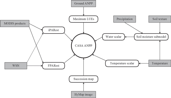
Figure 2. Framework for the estimation of Carnegie–Ames–Stanford approach (CASA) aboveground net primary productivity (ANPP) in this study. The CASA parameters included iPARest, estimated incident photosynthetically active radiation (PAR); FPARest, Fraction of absorbed PAR; temperature and water scalar, maximum light use efficiency (LUE), and ground ANPP as the sum of biomass increment and litterfall production. Details about the MODIS products are given in table 1. Data from wireless sensor network (WSN) were used to test the reliability of MODIS products. The succession map was derived to estimate ANPPCASA for each stage in the whole study area using a Hyperspectral MAPper technique (HyMAP).
Download figure:
Standard image High-resolution imageTable 1. Remote sensing datasets used in the current study.
| Role in this paper | Parameter | Dataset | Spatial resolution (m) |
|---|---|---|---|
| Succession mapping | — | HyMap | 15 |
| iPAR estimation | Instantaneous solar zenith | MOD04/MYD04 | 10 000 |
| Ångström exponent | MOD04/MYD04 | 10 000 | |
| Cloud top pressure | MOD06/MYD06 | 5000 | |
| Cloud optical thickness | MOD06/MYD06 | 10 000 | |
| FPAR estimation | NDVI | MOD13Q1 | 250 |
| EVI | MOD13Q1 | 250 |
We took advantage of a wireless sensor network (WSN) at the SRNP to continuously measure transmitted and absorbed PAR and meteorological variables. A WSN is a collection of independent nodes, each one measuring micro-meteorological variables that transmits such information via wireless to a data aggregator that in turn sends the data via cellular or satellite link to a cyberinfrastructure remote site where it is processed using analytical techniques (Pastorello et al 2011). WSN data (PAR) was collected in SRNP (mainly intermediate successional stage) from 06 March 2013 through 01 February 2015 (see supplementary section 1.2 for details) and were used to test the reliability of MODIS data in SRNP.
Specifically the main information used in this study was: instantaneous above canopy iPAR, PAR reflected by canopy, and PAR transmitted through canopy.
- (a)iPAR: is the amount of solar radiation in visible wavelength (0.4–0.7 μm) that can be absorbed by green canopy through photosynthesis processes (supplementary section 1.3). This study estimated regional 16 d integrated iPAR (iPARest) in SRNP using MODIS products based on the PARcalc method proposed by Van Laake and Sanchez-Azofeifa (2004, 2005) with some simplifications. One of the most important simplifications of the method is to ignore the presence of clouds during the dry season. The iPARest was evaluated by WSN measured iPAR (iPARmea) at the time span of 6 March 2013–1 February 2015.
- (b)FPAR: is the fraction of PAR absorbed by green vegetation. Long time series of FPAR (FPARest) were estimated from vegetation indices such as the normalized difference vegetation index (NDVI) and the enhanced vegetation index (EVI) (Prince and Goward 1995, Running et al 2000, Xiao et al 2004, Li et al 2007). We also examined relationships between measured FPAR (FPARmea) by WSNs, MODIS NDVI, and MODIS EVI using linear and logarithmic models from 6 March 2013 to 16 November 2014. The best fitting model was selected to produce long time series of FPARest (see supplementary section 1.4).
- (c)Maximum LUE (εmax_npp). The biome specific εmax_npp in the literature is derived by minimizing difference between ANPPCASA and ANPPmea (Field et al 1995, Ruimy et al 1999). Nevertheless, since TDFs in different successional stages present distinct species compositions (Kalacska et al 2004), we assigned a specific εmax_npp for early, intermediate, and late successional stages, by calculating the ratio of ANPPmea and estimated APAR
 using environmental scalars in the permanent plots based on equations (1)–(3), as follows:
 - (d)Temperature and water scalars (supplementary section 1.5). Temperature and water scalars limit conversion of solar radiation to ANPP in green vegetation. Temperature scalar, Tscalar(x, t), explains two patterns of plant acclimation to temperature: under extreme temperature and seasonal temperature swing. Water scalar, Wscalar(x, t), is a function of estimated and potential evapotranspiration, expressing water deficit from 0.0 to 1.0, where 1 is water saturation. Meteorological data (temperature and precipitation) was obtained from the meteorological station at SRNP.
- (e)Successional map. We produced a map of the successional stages in order to estimate ANPPCASA for early, intermediate, late successional stages in the whole SRNP area. Identification of successional stages employed a hyperspectral sub-pixel mapping technique called multiple criteria spectral mixture analysis (MCSMA) (Cao et al 2015). This technique was applied to a Hyperspectral MAPper (HyMap) image (Cocks et al 1998) acquired on March 2005. MCSMA was first applied by Cao et al (2015) to map secondary TDF succession at SRNP, and it proved to be very efficient in dealing with spectral variability in TDFs (supplementary section 1.6).

3. Results
3.1. Ground measured ANPP
Across successional stages, the intermediate stand had the greatest ANPPmea with an average biomass increment of 6.4 ± 2.5 Mg C ha−1 yr−1, and mean litterfall of 3.1 ± 1.0 Mg C ha−1 yr−1. Biomass increments and litterfall in late succession averaged 10.5 ± 1.2 Mg C ha−1 yr−1 and 5.9 ± 1.2 Mg C ha−1 yr−1, respectively. The early stage had a much lower biomass increment (5.2 ± 4.2 Mg C ha−1 yr−1) and litterfall (1.9 ± 1.5 Mg C ha−1 yr−1) (table 2). On average ANPPmea at SRNP was 7.1 Mg C ha−1 yr−1, with rates of carbon uptake of 3.6 Mg C ha−1 yr−1 in early stages, 9.5 Mg C ha−1 yr−1 in intermediate, and 8.2 Mg C ha−1 yr−1 in late succession.
Table 2. Mean values of biomass increment and litterfall production in 2007–2010 used to estimate of Annual Net Primary Productivity (ANPP) and derive εmax_npp in each successional stage at Santa Rosa National Park, Costa Rica.
| Stage | Plot | Biomass increment (Mg C ha−1) | Litterfall production (Mg C ha−1) | Measured ANPP (Mg C ha−1) | Estimated APAR·W_scalar·T_scalar (106 KJ ha−1) | Estimated εmax_npp (g C KJ−1) |
|---|---|---|---|---|---|---|
| Early | E1 | 4.56 | 1.53 | 6.09 | 32.87 | 0.19 |
| E2 | 3.82 | 1.43 | 5.25 | 32.81 | 0.16 | |
| E3 | 15.16 | 5.46 | 20.63 | 35.13 | 0.59 | |
| Average | 7.84 | 2.80 | 10.66 | 33.60 | 0.31 | |
| Intermediate | I1 | 14.78 | 11.40 | 26.18 | 34.64 | 0.76 |
| I2 | 26.67 | 10.41 | 37.08 | 36.53 | 1.02 | |
| I3 | 15.97 | 6.12 | 22.09 | 33.91 | 0.65 | |
| Average | 19.14 | 9.31 | 28.45 | 35.03 | 0.81 | |
| Late | L1 | 17.71 | 10.80 | 28.51 | 37.27 | 0.77 |
| L2 | 14.44 | 7.84 | 22.27 | 37.02 | 0.60 | |
| L3 | 14.88 | 7.71 | 22.59 | 36.44 | 0.62 | |
| Average | 15.67 | 8.87 | 24.46 | 36.91 | 0.66 | |
3.2. CASA ANPP
3.2.1. Estimated CASA parameters
3.2.1.1. Temporal dynamics and evaluation of estimated iPAR
The iPARest agreed robustly with iPARmea both in dry and wet seasons over the time series period (6 March 2013–1 February 2015) (figure 3(a)). The linear regression model also shows a strong relationship between iPARest and iPARmea (R2 = 0.83, y = 0.997x) (figure 3(b)). For each iPARest, absolute errors ranged 0.6% to 14.8% with average of 5.0%. The maximum individual error of 14.8% arises at the transition time from wet season to dry season at 19 December 2013, with a significant presence of brown downed leaves. Because of the constant presence of clouds, both 16 d total iPARest and 16 d total iPARmea in wet season were lower than in dry season (115 × 103 versus 159 × 103 KJ m−2).
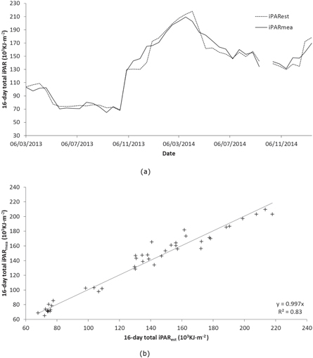
Figure 3. Comparison between 16 d estimated total iPAR (iPARest) and ground observed wireless sensor network derived iPAR (iPARmea) (from 6 March 2013 to 1 February 2015). Figure (a) demonstrates iPARest and iPARmea in a time series. Figure (b) fits a linear model between iPARest and iPARmea.
Download figure:
Standard image High-resolution image3.2.1.2. Relationship between MODIS vegetation indices and ground measured FPAR
Figure 4 shows the NDVI-FPARmea and EVI-FPARmea relationship using both a linear and a logarithmic regression model. The FPARmea increased from 0.5 in the middle of the dry season to 0.95 in wet season (figure 4(a)). Although the correlation between EVI and FPARmea could be considered high with a R2 = 0.83 (logarithmic model), versus R2 = 0.76 (linear model) (figure 4(c)); the NDVI-FPARmea relationship appears similar for both models (logarithmic model, R2 = 0.91; linear model, R2 = 0.90, figure 4(b)). Thus, posterior estimations of the FPARest for the modeling of ANPPCASA were based on the NDVI-FPARmea relationship instead of the EVI-FPARmea model.

Figure 4. Relationships between MODIS 16 d maximum vegetation indices and ground measured 16 d maximum FPAR (FPARmea) between 6 March 2013 and 16 November 2014. Figure (a) demonstrates MODIS NDVI, MODIS EVI, and FPARmea in a time series. Figure (b) is NDVI-FPARmea relationship. Figure (c) is EVI-FPARmea relationship.
Download figure:
Standard image High-resolution image3.2.1.3. Maximum LUE in different successional stages
Table 2 presents ANPPmea and estimated APAR · W_scalar·T_scalar for the 2007–2010 period, and the εmax_npp for each successional stage. Estimated εmax_npp showed similar pattern with ANPPmea. The highest εmax_npp was presented in intermediate stages (0.81 g C KJ−1), followed by late (0.66 g C KJ−1) and early (0.31 g C KJ−1) successions.
3.2.1.4. Seasonal dynamics of temperature and water scalars
Figure 5 presents boxplot of seasonal dynamics for the 16 d meteorological data and corresponding CASA scalar time series for complete year at SRNP. Each box was generated by summarizing corresponding meteorological data (12 July 2002 through 11 July 2014). Temperatures were stable across year at near the optimum value of 26.6 °C, with no significant differences between wet season and dry season (figure 5(b)). The temperature scalar also maintained high values greater than 0.9 (figure 5(d)). Precipitation, however, showed the two seasons characteristic in TDFs (figure 5(a)). The 16 d total precipitation was maximized in wet season, with almost no precipitation recorded in dry season. Precipitation presented its greatest inter-annual variation during the wet season, with a maximum standard deviation of 22.3 cm in late September (from 273th to 289th day of the year; not shown in figures). The water scalar had a similar pattern with precipitation. The land surface at SRNP became gradually water stressed as the dry season proceeded, despite that being relieved by occasional precipitation for instance on 03 April 2009 (6.7 cm) (figure 5(c)).

Figure 5. Boxplots for meteorological data and scalars in 2002–2013 at SRNP. Figure (a) precipitation. Figure (b) temperature. Figure (c) water scalar. Figure (d) temperature scalar.
Download figure:
Standard image High-resolution image3.2.2. Total and seasonal ANPPCASA in different successional stages
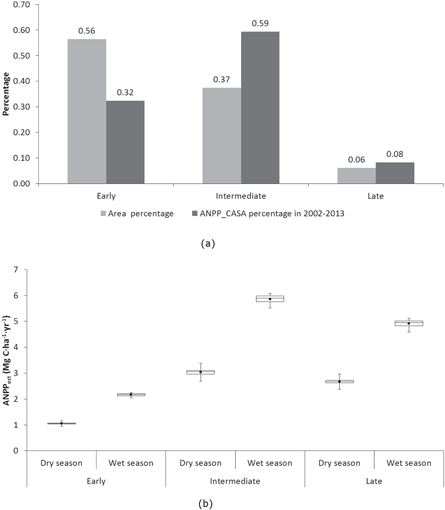
We produced successional maps of early, intermediate, and late successional forests at SRNP by using the MCSMA to derive ANPPCASA for each stage. Figure 6(a) compares area of TDFs in each successional stage at SRNP against their average ANPPCASA (2002–2013). At SRNP, early successional stages comprised 56% of the total area, followed by intermediate successional stages with 37%. In contrast, early and intermediate successional stages comprised 32% and 59% of the total ANPPCASA respectively. Both fractions of area and ANPPCASA in late successional stages were small. Figure 6(b) illustrates the variation of the ANPPCASA in the dry and wet seasons (December–April; May–November). Each box (e.g., ANPPCASA of early successional stages dry season) was generated using data from 2002 to 2013. For all successional stages, ANPPCASA in the dry season (early: 1.06 Mg C ha−1 yr−1; intermediate: 3.04 Mg C ha−1 yr−1; late: 2.67 Mg C ha−1 yr−1) was half of ANPPCASA in the wet season (early: 2.17 Mg C ha−1 yr−1; intermediate: 5.86 Mg C ha−1 yr−1; late: 4.91 Mg C ha−1 yr−1). For each year, the ANPPCASA of intermediate stages (8.90 Mg C ha−1 yr−1) was higher than ANPPCASA of late successional stages (7.59 Mg C ha−1 yr−1), and 2.8 times higher than ANPPCASA of early successional stages (3.22 Mg C ha−1 yr−1) (figure 6).
Figure 6. CASA ANPP (ANPPCASA) in 2002–2013 at SRNP. Figure (a) presents area percentage (derived based on HyMap image acquired on March 2005 at SRNP) and ANPPCASA percentage (averaged across 2002–2013) of early, intermediate, and late successional stages. Figure (b) presents the annual ANPPCASA in dry and wet seasons of early, intermediate, and late successional stages in 2002–2013.
Download figure:
Standard image High-resolution image
4. Discussion
4.1. Comparison with other ANPP studies in TDFs
Our estimates of ANPPmea from ground data are similar to another study conducted in Costa Rica' TDFs. Waring et al (2015) reported rates of carbon gain from biomass increments and litterfall production 4.04 Mg C ha−1 yr−1 to 5.73 Mg C ha−1 yr−1 on stands of 15–65 years of age since land abandonment. For TDFs in other regions, Lugo and Murphy (1986) estimated ANPPmea in Puerto Rico's Guanica forest as 3.45 Mg C ha−1 yr−1 by summing forest biomass increments and litterfall production. Martinez-Yrizar et al (1996) reported ANPPmea of 3.06, 3.14, and 4.04 Mg C ha−1 yr−1 at three plots with decreasing elevations within a watershed at Chamela Biological Station, Mexico. Their measurements, however, included other two ANPP components leaf herbivory and understory production. When only biomass increments and litterfall production were considered, ANPPmea for the three plots at Chamela Biological Station were 2.65, 2.74, and 3.56 Mg C ha−1 yr−1, respectively, which are comparable to our measurements. The variation on the upper limits of ANPP among existing studies and with our results could be explained by higher water availability at SRNP (mean annual precipitation; Guanica: 860 mm yr−1; Chamela: 707 mm yr−1; SRNP: 1390.8 mm yr−1).
4.2. Key parameters estimation in CASA
The relative lower correlation between EVI and FPARmea could be partially a result of the high sensitivity of MODIS EVI to the Sun-sensor geometry effect and canopy structure (Morton et al 2014). However, other studies have found better correlations between MODIS NDVI and LAI than using MODIS EVI in deciduous forests (Wang et al 2005) and in TDFs. Silveira et al (2007) for example, found that the best vegetation index for mapping vegetation classes in deciduous and semi-deciduous forests and Cerrado (Brazilian savannas) were obtained using the MODIS NDVI images than using MODIS EVI. This may be due to the fact that EVI tends to be more sensitive to NIR reflectance (Huete et al 1997) since it is more responsive to canopy structural variations, including LAI, canopy type, and canopy architecture (Huete et al 2002), whereas the NDVI is more chlorophyll sensitive (Huete et al 2002). This might be the reason why NDVI works better in dry forests compared to wet forests, since dry forests have a very heterogeneous forest canopy, with greater canopy openness and lower LAI even in the wet season (Arroyo-Mora et al 2005, Kalacska et al 2005b, Castillo-Núñez et al 2011).
4.3. Dominant ANPP drivers in TDFs
Meteorological conditions dominate seasonal ANPP patterns at SRNP. Temperatures were stable at near optimum values across the year, making it an insignificant factor in ANPPCASA estimation. Precipitation and FPAR exhibited opposite seasonal patterns to iPAR because of occurrences of rainfall and cloud cover. Precipitation greatly varied between dry and wet seasons. It is not surprising that abundant precipitation in the wet season promotes high ANPPCASA because water availability is one of the main controls of leaf production and photosynthesis in TDFs (Jaramillo et al 2011). Our ANPPCASA estimations showed TDFs sustaining photosynthesis even in the driest months at SRNP. This is probably related with changes in species composition across successional stages, with more than 80% of plants losing their leaves in the dry season, while only 30%–50% deciduous species in older stages of succession (Kalacska et al 2004, Arroyo-Mora et al 2005). Several plant species in TDFs have evolved different adaptive mechanisms with deep roots ensuring water supply for photosynthesis (Nepstad et al 1994). For example, woody vines, which are specially abundant on intermediate TDFs stages of succession, uptake more water than trees during water stress periods (Chen et al 2015) and as such tend to drop their leaves later in the dry season (Kalacska et al 2005a).
FPAR, which expresses the forest canopy structure and greenness (Arroyo-Mora et al 2005, Kalacska et al 2007), had a similar seasonal pattern with the water scalar in TDFs with high values in wet season and low values in dry season. This confirms the importance of rainfall in the leaf phenology of TDFs. The cyclical regimes of precipitation largely drive leaf flushing and falling events in secondary TDFs across different latitudes (Martha et al 2013). In our study, seasonal variability of ANPPCASA from iPAR was dominated by FPAR and the water scalar, and values of ANPPCASA during wet season were twice as much as in dry season. This differs from other studies in tropical environments that concluded that iPAR was the most influential climatic factor for primary productivity (Imoto et al 2010).
Assuming that SRNP experienced homogeneous meteorological conditions (iPARest, temperature, precipitation) across study plots, variations in ANPPCASA originated from differences in FPARest and εmax_npp across successional stages (see equations (1)–(3)), likely explained by differences in species composition and stem density. At tree level, εmax_npp is a function of tree physiological processes and allometry, and in turn, a function of tree species. TDFs in late successional stages are dominated by shade-tolerant species with lower growth rates, while TDFs in early and intermediate stages have greater abundance of pioneer species that prefer full sunlight conditions with faster growth rates (Carvajal-Vanegas and Calvo-Alvarado 2013). As a result, early and intermediate stages present higher tree diameter increments (early: 1.6 mm tree−1 yr−1 versus intermediate: 2.2 mm tree−1 yr−1) than in late successional stages (1.2 mm tree−1 yr−1) (Carvajal-Vanegas and Calvo-Alvarado 2013). At regional level, εmax_npp is further a function of stem density (Kalacska et al 2005b), promoting TDFs to reach their highest ANPP (mainly by litterfall production) in intermediate and late stages (table 2). This highlights the important role of intermediate and late successional stages in carbon sequestration, since these two successional stages have a greater ability to convert absorbed solar radiation into plant primary productivity (intermediate: 0.81 g C KJ−1 versus late: 0.66 g C KJ−1) than early successional stage (0.31 g C KJ−1).
Furthermore, FPAR reflects canopy differences between different successional stages. Older successional stages with lower canopy openness and deciduousness have higher FPAR than younger successional stages (Arroyo-Mora et al 2005). For instance, TDFs in early succession were dominated by short trees, shrubs and grasses, which translated into higher canopy openness and lower greenness (Sanchez-Azofeifa et al 2009), and thus had lower FPARest compared to intermediate and late successional stages. It has also been reported that open canopies in TDFs are more vulnerable to wind and storm effects, losing their leaves faster and sooner in dry season than closer canopies (Jaramillo et al 2011, Calvo-Alvarado et al 2012). The successional effects from εmax_npp and FPARest together explained that, early successional stages that currently represented more than half of the total area of SRNP accounted for only one third of the total ANPPCASA, indicating that TDFs ANPP are more influenced by forest succession and species composition rather than forest area and forest extent.
The dominating role of precipitation in seasonal ANPP variation of TDFs highlights the need to collect more accurate and spatially explicit precipitation or soil moisture data in PEMs, despite that only one meteorological station was available at SRNP for our study. It is also important to consider the influence of structure and species composition of forest stands on ANPP in TDFs. Our model indicates that species composition explained the variation of ANPP. Other studies in TDFs in Costa Rica have found that these changes in species composition across successional stages may be explained not only by previous land use (e.g., stand age), but also by soil properties, including soil moisture (Becknell and Powers 2014). The water availability in our model relies mostly on rainfall, and we still lack a thorough understanding about the role of soil properties on ANPP. Future studies should explore the direct and indirect effects of soil on ANPP, via changes in species composition or by assessing the seasonal variation in soil moisture and its potential impact on rates of ANPP.
5. Conclusion
We explored the potential of the CASA model for estimating ANPP in TDFs. We found two dominant drivers for ANPP in TDFs, precipitation and successional stage (forest age). Specifically, the FPAR and water scalar term in CASA are indicators of precipitation controls in phenology process and photosynthesis process, respectively. The maximum LUE (εmax_npp) reflects the differences of species composition (tree species) and forest structure (tree diameter, diameter increments, and tree density) in different successional stages. FPAR as a proxy of canopy openness and greenness is also a function of successional stage. Furthermore, despite that the iPAR appears to be the main driver for the ANPP in many tropical ecosystems, its impacts on ANPP is surpassed by precipitation at our TDF study site. Future work should focus on applying PEMs in other TDFs sites to consolidate findings from this paper.
Our study assesses a remote sensing methodology to estimate ANPP in TDFs as a tool to monitor changes in carbon capture and uptake at regional scales. Our results may facilitate the development of management policies of regenerating pastures, since they identify the main ANPP drivers in TDFs and their impacts from climate and previous land transformation at local and regional scales.
Acknowledgments
This work was carried out with the aid of a grant from the Inter-American Institute for Global Change Research (IAI) CRN3 025 which is supported by the National Science Foundation of the United States (Grant GEO-1128040). We acknowledge the support provided by the National Science and Engineering Research Council of Canada (NSERC-Discovery Grant Program). We would also like to thank Waldy Medina for supplying maps of Santa Rosa National Park.