

Abstract
Large-scale airborne lidar data collections can be used to generate high-resolution forest aboveground biomass maps at the state level and beyond as demonstrated in early phases of NASA's Carbon Monitoring System program. While products like aboveground biomass maps derived from these leaf-off lidar datasets each can meet state- or substate-level measurement requirements individually, combining them over multiple jurisdictions does not guarantee the consistency required in forest carbon planning, trading and reporting schemes. In this study, we refine a multi-state level forest carbon monitoring framework that addresses these spatial inconsistencies caused by variability in data quality and modeling techniques. This work is built upon our long term efforts to link airborne lidar, National Agricultural Imagery Program imagery and USDA Forest Service Forest Inventory and Analysis plot measurements for high-resolution forest aboveground biomass mapping. Compared with machine learning algorithms (r2 = 0.38, bias = −2.3, RMSE = 45.2 Mg ha−1), the use of a linear model is not only able to maintain a good prediction accuracy of aboveground biomass density (r2 = 0.32, bias = 4.0, RMSE = 49.4 Mg ha−1) but largely mitigates problems related to variability in data quality. Our latest effort has led to the generation of a consistent 30 m pixel forest aboveground carbon map covering 11 states in the Regional Greenhouse Gas Initiative region of the USA. Such an approach can directly contribute to the formation of a cohesive forest carbon accounting system at national and even international levels, especially via future integrations with NASA's spaceborne lidar missions.
Export citation and abstract BibTeX RIS

Original content from this work may be used under the terms of the Creative Commons Attribution 4.0 license. Any further distribution of this work must maintain attribution to the author(s) and the title of the work, journal citation and DOI.
1. Introduction
A rising interest in using forests as a nature-based solution to combat climate change has prompted multiple forest carbon initiatives at regional, national and international levels. Tremendous progress has been made over the past few years with multiple afforestation and reforestation projects operating or planned across different strategic areas around the world (Griscom et al 2017). One common and ever-increasing requirement from these initiatives is a precise measurement of current forest carbon stocks (Goetz and Dubayah 2011). It is thus of critical importance to generate high-resolution baseline forest carbon maps within the context of carbon monitoring and climate change mitigation efforts to support policy-relevant forestry activities (Houghton 2013, UNFCCC 2015).
Airborne lidar can be used to accurately map the spatial distribution of canopy structure and aboveground biomass, and has played an instrumental role in high-resolution forest carbon mapping initiatives (Duncanson et al 2015, Nilsson et al 2017, Zhao et al 2018). While most of these forestry lidar projects are targeted at smaller areas, more recent studies have also pioneered statewide forest carbon mapping efforts by leveraging the extensive and increasing coverage of leaf-off topographic lidar campaigns (Chen and McRoberts 2016, Huang et al 2019). These large-area forest biomass mapping efforts, including our previous studies in the US states of Maryland, Pennsylvania and Delaware (hereafter, MD-DE-PA) as part of NASA's Carbon Monitoring System (CMS) (Huang et al 2015, 2019, Hurtt et al 2019), have been able to achieve impressive performance, such as a root mean square error (RMSE) of 30–50 Mg ha−1, which is a level generally comparable to many leaf-on forestry lidar applications.
However, challenges remain in the use of uncoordinated lidar data collections for high-resolution forest carbon mapping at state and interstate levels (Lu et al 2016, Mcroberts et al 2018). Our MD-DE-PA study focused on the compilation of lidar collections from multiple agencies and the improvement of project-level statistical models (Huang et al 2019), but did not yet resolve issues related to inconsistent spatial data structure and quality, variability of methods, and as well as output quality across regions. These problems appear less obvious within small geographical domains such as a U.S. county or multi-county region, but their impact on interstate forest carbon mapping becomes more evident when attempting to produce carbon maps across the Northeastern and Mid-Atlantic US. In particular, spatial discontinuities become quite apparent when attempting to combine pixel-level forest aboveground biomass estimates across jurisdictional boundaries, which typically divide lidar data collection campaigns.
In this paper we aim to resolve these emerging challenges in statewide lidar-based forest biomass mapping initiatives. We provide an updated observation and modeling framework across ten member states of the Regional Greenhouse Gas Initiative (RGGI), the nation's first mandated cap-and-trade program for CO2 emissions, plus Pennsylvania, which is expected to participate in RGGI by 2022 (www.rggi.org). Here, we focus on the investigation of regional spatial discrepancies and seek a strategy that balances local optimization and global consistency, a key element in interstate accounting and trading policy (Lamb et al 2020). We also share experiences and provide recommendations for comparing and compiling multi-campaign forest biomass datasets. Finally, we generate a high-resolution mapping framework to establish policy-relevant forest carbon baselines that can be expanded to the entire nation.
2. Methods
The overall methodology is largely inherited from our earlier efforts over the U.S. states of Maryland, Delaware and Pennsylvania (Huang et al 2015, 2019). It includes inputs from forest inventory and remote sensing datasets, as described below. Here we optimize our MD-DE-PA workflows by focusing on recent lidar and inventory datasets from the New England area. More detailed descriptions of our entire study area can be found in a parallel study submitted to the same issue (Ma et al 2020).
2.1. Remote sensing input
High-resolution normalized difference surface model (nDSM) and tree canopy cover raster datasets, both at 1 m pixel nominal resolution, served as the fundamental remote sensing inputs for generating aboveground forest carbon estimates. The nDSM can be thought of as a 1 m canopy height map that was derived from discrete return lidar data collected by various local, state and national agencies. The tree canopy cover map was generated from lidar data and high-resolution imagery from the National Agricultural Imagery Program (NAIP) using an object-based approach (O'Neil-Dunne et al 2014). A set of forestry metrics (Huang et al 2019), such as percentile heights and canopy cover, were calculated from the two inputs at 30 m pixel resolution in alignment with a National Land Cover Dataset (NLCD 2011) (Homer et al 2015).
2.2. Field inventory input
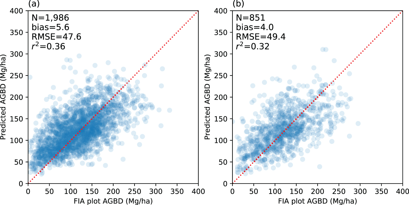
Forest inventory data from the USDA Forest Service's Forest Inventory and Analysis Program (FIA) were used for calibration and validation of our carbon maps. While we collected additional inventory data for our MD-DE-PA work, the current study relied solely on FIA data. This is partly due to limited resources for additional field campaigns over the entire RGGI region, but more importantly, because in our previous work, comparisons of FIA and ancillary field datasets indicated a reasonably good agreement with major uncertainty in aboveground biomass density (AGBD) estimation originating from low-quality lidar data and limited model performance (i.e. RMSE of 50–60 Mg ha−1) (Huang et al 2019). In addition, leveraging a single dataset with consistent methods and national scope, like FIA, will facilitate future national expansion of our baseline mapping efforts. We created a subset of the FIA database based on compatible acquisition times between field and lidar data, using the FIA data collection cycle that straddled the nominal year of lidar acquisition. From the subset of acceptable training and validation data, we randomly selected 70% of the plots for training and used the remaining 30% for validation (N = 1986 and 851 respectively). Note we only used FIA plots that were labeled as 100% accessible forest, as plots that were partially inaccessible or contained non-forest land might have trees that are not measured and therefore not serve as suitable training or validation data. This practice, however, narrowed the definition of our measurement target, i.e. from AGBD per unit land area to AGBD of forested area only. Failing to address this discrepancy can lead to an improper interpretation of our results especially over partially forested land parcel (e.g. 50% forest and 50% bare ground in a hectare).
2.3. Biomass modeling
We successfully employed a set of Random Forest models in different phases in our MD-DE-PA work, but concerns about overfitting led us to assess linear models aiming to increase both pixel-level accuracy and spatial consistency in AGBD estimation. This is because a linear model typically has better model stability and geographic transferability with a straightforward data structure (Zhao et al 2018). In addition, we directly modeled measurement error using a Bayesian approach, accounting for possible biases in leaf-off lidar data (e.g. underestimation of canopy height). For both methods, model fit was compared against the data used to construct models as well as the validation dataset. For the Random Forest model, relative importance among predictor variables was assessed based on the mean decrease impurity (i.e. Gini importance). More technical details about the pixel-level estimation of AGBD and its uncertainty can be found in the supplement.
3. Results
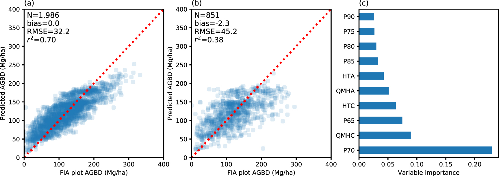
The Random Forest model explained about 70% variability of the data used to build the AGBD model over the New England region (figure 1(a)), a level similar to our findings in MD-DE-PA (Huang et al 2019). However, its accuracy dropped substantially when applied over the validation dataset (figure 1(b)). Middle-level canopy height metrics, such as P70 or P75 (i.e. the 75th percentile of lidar canopy height within a pixel), typically achieved the highest correlations with AGBD (P70) or identified as the most important features (P75) in the Random Forest model (figures 1(c) and S1 which is available online at stacks.iop.org/ERL/16/035011/mmedia). A saturation effect described in our previous studies (Huang et al 2019) took place in our experiment with an underestimate in the high AGBD range and an overestimate at the low end (figures 1(a) and (b)). There also appeared to be a cutoff line from the model with no prediction over 200 Mg ha−1 even though there were many field observations exceeding that threshold.

Figure 1. Comparison of Random Forest-model predicted and FIA-based biomass from the calibration dataset (a) (70% data) and validation dataset (b) (30% with-hold data). While P70 has the highest feature importance score in the model (c), it is highly correlated with some other canopy metrics (e.g. P90, mean height and quadratic mean height; figure S1). Multicollinearity and overfitting issues therefore drastically lower the prediction accuracy in the independent validation dataset.
Download figure:
Standard image High-resolution imageThe impact of inconsistency in nDSM data properties across jurisdictional boundaries was less obvious during the model development phase, but became more pronounced when the models were applied and the verisimilitude of maps was assessed. Figure 2 provided one example of spatial inconsistency at the state boundaries of Connecticut (CT), Massachusetts (MA) and Rhode Island (RI) as the state-level data were collected from different campaigns. While P70 was the single best predictor of AGBD shown in the Random Forest model, it was less than ideal for baseline mapping and created artifacts in spatial distribution of AGBD estimation particularly at the intersection area of multiple airborne lidar collections. By contrast, higher percentile metrics (e.g. P95 or P100), despite a slightly lower correlation with AGBD (figure S1), presented a much more consistent spatial pattern across these boundaries, making them better candidates for use as predictor variables in empirical biomass models in our methods.
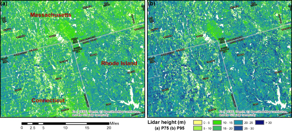
Figure 2. An example of 30 m lidar-based height metrics at the borders of CT, MA and RI. Juxtaposition of lidar data collected from different campaigns has a much greater impact on middle-level canopy percentiles (e.g. P75 in panel a) than on higher ones (e.g. P95 in panel b). For example, RI seems to have a systematically higher P75 than MA, and CT data suffer from possible observation artifacts between flight lines (apparent striping). By contrast, these issues were less obvious for P95 that exhibited higher spatial consistency.
Download figure:
Standard image High-resolution imageResults of the Bayesian model supported the use of linear models in AGBD prediction and provided a quantitate assessment of lidar measurement error as well (figures 3 and S2, S3). Our error model in a log-log hierarchical linear model suggested an underestimate of 2.95 ± 0.40 m in P95 relative to true canopy height based on Markov chain Monte Carlo (MCMC) simulation results (figure S4). Use of P100 could reduce the potential bias to 1.21 m (figure S5) but we did not use it to generate the final biomass product because of its lower correlation with AGBD than that of P95 (figure S1). These relationships could also vary across different land cover types, ranging from the lowest value of 0.39 m in wetlands to 4.35 m in deciduous forests and 5.03 m in evergreen forests (figures S7 and S8). Compared with the Random Forest model, the linear models had a lower accuracy for the calibration data but showed a comparable validation accuracy without evidence of overfitting (figures 3 and S2, S3). No obvious saturation effect or spatial inconsistency at campaign boundaries was found in subsequent model or map diagnoses, suggesting a high geographic transferability and robustness to lidar measurement variability (figure 4(a)).
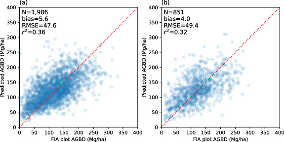
Figure 3. Comparison of a linear log-log model predicted and FIA-based biomass with the same data used in figure 1. Compared with the Random Forest model (figure 1), there is less evidence of overfitting, as the calibration and validation statistics are more similar.
Download figure:
Standard image High-resolution image
Figure 4. Lidar-based AGBD maps (30 m resolution) over the New England region. Panel (a) corresponds to the mean of the posterior distribution sampled from an MCMC model. Panel (b) shows the AGBD estimate over entire pixel adjusted by canopy cover (i.e. AGBD multiplied by canopy cover percentage). Despite similar forest carbon density values between forests and suburban area, their total carbon stock per unit area can differ by one order of magnitude, highlighting the requirement for high-resolution mapping of both forest biomass density and extent in carbon accounting framework.
Download figure:
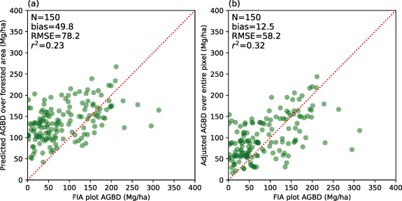
Standard image High-resolution imageThe use of P95 alone, as an approximation of maximum canopy height, could however lead to confounding results over sparsely vegetated area. For instance, it appeared to inflate the AGBD over urban developments, or in areas with trees outside forests (TOF), especially when aggregated at resolutions corresponding to predictions from ecosystem models (i.e. 90 m) (Ma et al 2020, Hurtt et al 2019). This was expected because the FIA plot data used to calibrate and validate our AGBD maps were limited to pure forested plots, a situation would tend to lead to predictions of higher-than-expected biomass in low-biomass areas. In order to address this deficiency, we integrated an independent forest percentage cover map to account for the difference from 100% forested area, as shown in figures 4(b) and 5. However, this adjustment may also introduce additional uncertainty subject to the quality of the forest percentage cover map generated from lidar and NAIP imagery.
Figure 5. Comparison over developed urban area between model-predicted AGBD and all FIA plot-level estimates at 90 m resolution. Panel (a) shows a relative overestimation of our empirical lidar model because it does not account for the percentage of forest coverage in a pixel. An adjustment using canopy cover in panel (b) can partly correct this effect particularly at the low range (0–100 Mg ha−1).
Download figure:
Standard image High-resolution image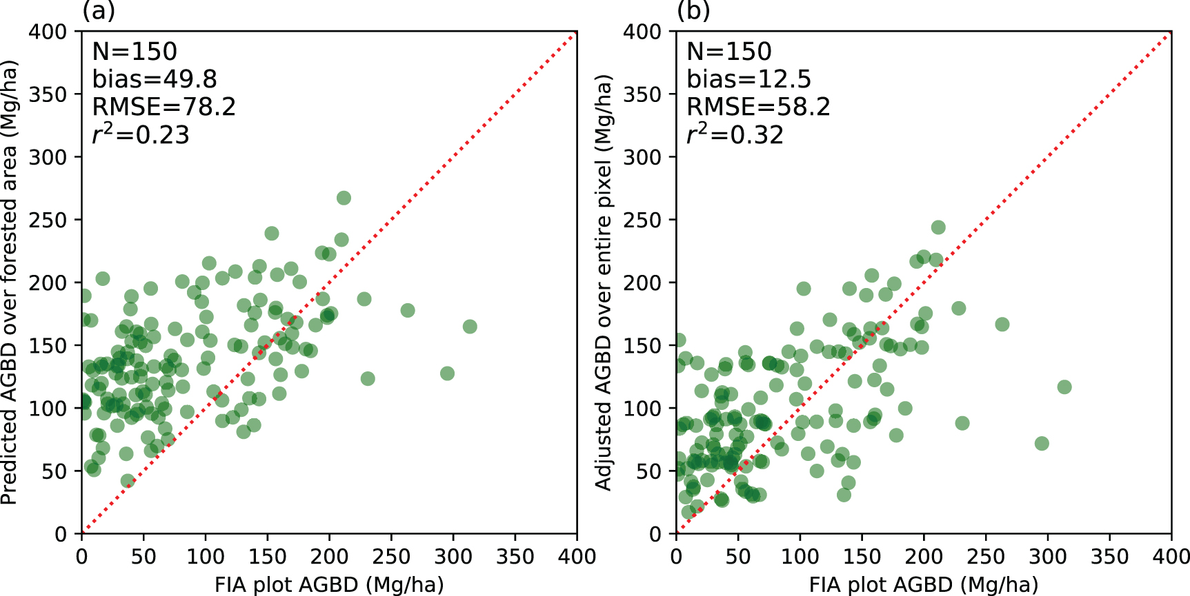
4. Discussion
Airborne lidar has played a pivotal role in mapping 3D vegetation structure and aboveground biomass, and serves as foundational reference data for many NASA CMS projects. However, most of these lidar datasets used-to-date were collected during leaf-off conditions, under low point density, and with the primary goal of terrain mapping. The variability found in these lower-quality datasets led to two major problems when generating high-resolution forest carbon baseline map over broad geographic domains: spatial inconsistency and poor model transferability. This study specifically addressed these two critical issues while building upon our nearly decade-long mapping progress within the RGGI region; we started with two counties in the state of Maryland, progressed to MD-DE-PA level, and finally created maps over nearly the entire RGGI domain (Huang et al 2015, 2019). In the early phases of the project, biomass maps were derived at either county level or for individual airborne lidar campaigns and then mosaicked together to generate a statewide seamless map, a strategy widely adopted by the lidar and biomass mapping community. While these mosaics can individually meet threshold accuracy requirements, a simple aggregation of these high-resolution biomass maps does not guarantee a consistent estimate over the entire domain of interest, especially at a spatially explicit level. Inconsistencies were typically caused by variability of lidar data characteristics and processing approaches for different campaigns; this can result in spatial irregularities as can be seen in the example of state borders shown in figure 2. These inconsistencies had the greatest impact on the middle and lower portions of canopy structure (e.g. P50–80), which usually achieved the best empirical relationship with forest biomass. Notably it also underestimated true canopy height, as found in previous studies (Wasser et al 2013, White et al 2015). These types of lidar measurement inconsistencies carried over into maps of modeled biomass, particularly when using predictor variables, like P70 or 75, that were more sensitive to these types of artifacts.
4.1. Mitigation strategies
Our approach, based on the Bayesian inference framework, provided improvements to previous methods in various ways. First, inconsistency of lidar collection was largely mitigated through the use of noise-robust metrics and an error model. High-end canopy height metrics such as P95 showed a higher resilience to data collection artifacts such as those shown in figure 2. Our error model at the pixel level, using a classical Gaussian model, identified an average bias of −3.6 m between P95 and true canopy height in the applied lidar datasets and added further robustness in the modeling process (figure S4). This result was consistent with previous findings that leaf-off low-density lidar tended to underestimate actual heights by frequently missing canopy tops. While P100 reached a closer agreement with true height (figure S5), we chose not to use it in our baseline estimate because of its lower correlation with biomass density (figure S1). This decision was also based on our experience that P100 was more prone to corruption by environmental noise and outliers. Second, the use of a linear model exploring the relationship between biomass density and canopy height minimized the overfitting problem. Machine learning algorithms, such as Random Forest, can better explore the multidimensional feature space and select the best combination for a given training dataset. However, these models do not necessarily generate the best predictions with independent validation datasets, as shown in the literature (Zhao et al 2018) and in our results as well (figure 1). Meanwhile, some of the most important predictor variables identified by Random Forest (e.g. P75) turned out to be more susceptible to artifacts in the lidar data. Together, these factors increased the risk of overfitting, degraded pixel-level accuracy and limited model geographic transferability. By contrast, the use of a linear model overcame these problems and generated predictions spatially consistent across the entire region. Despite a simpler data scheme and model structure, its accuracy level was comparable to or even exceeded more advanced models used in previous studies (with RMSE of 40–60 Mg ha−1). Finally, our Bayesian framework and MCMC implementation generated a straightforward interpretation. The posterior distribution of the model output provided a convenient, intuitive estimate of pixel-level uncertainty (figure S4). Its hierarchical model structure also provided a greater freedom to improve current estimates by incorporating either additional predictor variables from other data sources (e.g. forest type in figures S7–9), or independent biomass estimates in the future.
Another important update in our modeling framework was an explicit separation of biomass density between forest and non-forested area. In this study we modeled AGBD only over forested areas, and included a forest cover map to adjust AGBD estimates for partially forested areas. We used this two-step approach because non-forested or partially-forested FIA plots were less than ideal for developing our statistical biomass models: trees in areas not meeting FIA's definition of forest were not measured, causing a degradation of the relationship between tree biomass and lidar tree height metrics upon which our models rely (Huang et al 2015). Our results supported this hypothesis and the model performance was in much better alignment with FIA's primary measurement focus on forests than partially vegetated land. Their performance discrepancy became most evident in urban environments with sparsely-distributed large trees. It was because these trees' individual biomass contributions could be very high but the biomass density value was low when averaged over a mapping unit with low forest coverage. Our use of a high-resolution canopy cover map mitigated this problem to a great extent (figures 4(b) and 5), but did not fully resolve the issue. For example, we noticed an underestimation over part of CT along a lidar flight line that could be caused by the spatially varying precision of canopy cover maps generated from lidar and NAIP imagery. While it was possible to update the AGBD estimate with a refined forest extent product, we chose not to in this case because, over most of the RGGI region, our current high-resolution map exceeded the performance of other canopy cover products readily available from satellite imagery or synthetic aperture radar (O'Neil-Dunne et al 2014) and the choice between them would likely have a relatively small impact on the total estimated biomass. Our baseline estimates over areas with a lot of TOF should therefore be used with caution. A full assessment of TOF biomass would require an independent mapping initiative targeting the complicated TOF landscape found in urban areas, or possibly through object-based identification of individual trees and the aid of FIA's urban program (Johnson et al 2014).
4.2. Limitations
Despite these mitigation efforts, our approach cannot fully overcome some limitations inherent in current mapping efforts when using FIA data alone. First, not all lidar and FIA data are collected in the same year given insufficient availability of lidar coverage. The relaxation of their temporal overlapping to a 5 year FIA measurement cycle is a compromise strategy and inevitably introduces additional uncertainty in our biomass models. It is possible though to correct this temporal difference using prognostic ecosystem models that predicts annual biomass changes (Hurtt et al 2019, Ma et al 2020). Geolocation error in FIA plot, subject to survey protocol and quality of GPS used in the field, adds a second level of uncertainty and is more difficulty to adjust. When compounded with the edge effect caused by smaller size of FIA plots, it further weakens the relationship between remote sensing signal and field biomass measurement. A more robust strategy, as shown in recent regional studies (Deo et al 2017, Hudak et al 2020), is to first lay out additional forest inventory plots of sub-meter level geolocation accuracy for model calibration, and then applies FIA plots for independent validation purpose. Similar pilot projects continue to expand and generate high quality lidar-field pairs ideal for developing regional calibration equations of aboveground biomass, and will bring tremendous benefits to our future mapping efforts once spanning all forest types and environmental gradients.
In summary, results of this study represent the first baseline map of forest aboveground biomass across the RGGI region with unprecedented geographic extent and resolution. Moving forward, these estimates will be continuously updated as new lidar datasets become available and FIA plots are re-measured, and gradually fill up current observation gaps over the entire US. Our previous biomass mapping experience suggests that more technical difficulties are likely to emerge in this process. One potential challenge, for example, is how to best reconcile forest biomass estimates from multiple ongoing forest carbon projects as we have started seeing increased spatial discrepancies within our own multi-year project as the methods evolve. A consistent baseline estimate framework across multiple projects is of critical importance for carbon mitigation polices and planning at regional, state, national and international levels (Lamb et al 2020). This framework also has a direct relevance to NASA's ongoing lidar satellites, GEDI and ICESat-2, both of which have the capacity to generate global forest structure and biomass products (Neuenschwander and Magruder 2019, Dubayah et al 2020). A better integration of these satellite observations to high-resolution biomass reference maps, either through direct comparison or via a data fusion technique, can ultimately help improve our baseline estimates of national and global forest carbon circa 2020.
5. Conclusions
Airborne lidar data collection efforts are continuing throughout the US, and have the potential to generate a nationwide high-resolution forest carbon baseline map within this decade. A simple combination of these lidar datasets, however, may not maintain the quality and precision required for forest carbon accounting initiatives. It is thus necessary to not only address lidar data collection and processing variability, but more importantly, to develop modeling strategies for generating a consistent aboveground biomass product as demonstrated in this study. Our methodology over the RGGI domain directly addresses this issue by accounting for some of the most critical factors in high-resolution forest carbon mapping. The forest height and carbon map developed over the RGGI domain provides a bottom-up reference and facilitates predictions of long-term carbon sequestration potential, and together, they form a valuable baseline for climate mitigation planning. Meanwhile, its success demonstrates one potential pathway for generating a seamless forest carbon mapping system across the pixel-, county-, state- and multistate-levels. Ultimately, our analyses and related products can fold into a continental and global forest carbon monitoring system through synergies with the upcoming biomass estimates from multiple satellite missions.
Acknowledgments
We gratefully acknowledge the support of the NASA Carbon Monitoring System program, Terrestrial Ecology program, New Investigator program, and Interdisciplinary Research in Earth Science program (NNX12AN07G, NNX14AP12G, 80NSSC18K0708 and 80NSSC17K0710). We also acknowledge in-kind support from the US Department of Agriculture, Forest Service, Forest Inventory and Analysis Program.
Data availability statement
The data that support the findings of this study are available upon reasonable request from the authors and can also be found using the following link https://doi.org/10.3334/ORNLDAAC/1854.