


Abstract
Building on one decade of theory and methodology maturation, we investigate the coherent and incoherent components of the response of the Martian surface to nadir-looking orbital radar. We apply a reflectometry technique known as radar statistical reconnaissance to Mars Reconnaissance Orbiter Shallow Radar data over a test region with a large dynamic range in echo strength. This technique provides a set of statistical parameters describing the heterogeneity of the surface and near-surface structure, presumably at a scale of ∼15 m. We discuss the physical meanings of these parameters related to surface and near-surface properties. Most (but not all) investigated terrains have a dominantly coherent surface return, a characteristic that is not necessarily indicative of a smooth surface. The observed behavior of the coherent and incoherent power components of the echo matches signal growth with increasing surface roughness. This finding allows us to identify smooth and level terrains that we use as a reference to approximate the surface height and slope variations of other regions. Nearly systematic mismatches between the SHARAD and MOLA-pulse-width roughness illustrate the complementarity of these data sets from their respective sensitivity range, and advocate for the use of self-affine radar backscattering models to account for roughness variations at different scales. Our methodology provides a wealth of surface properties assessment based on radar scattering with quasi-global coverage, without a dependence on other data, and at a decametric horizontal scale relevant to subregional geology investigation and landing site reconnaissance.
Export citation and abstract BibTeX RIS

Original content from this work may be used under the terms of the Creative Commons Attribution 4.0 licence. Any further distribution of this work must maintain attribution to the author(s) and the title of the work, journal citation and DOI.
1. Introduction
The information contained in the surface echo return of nadir-looking radar data can be used to classify, outline, and characterize planetary surfaces by being sensitive to a combination of properties unique to radar instruments. However, the contributions of the near-surface composition, structure, and surface roughness are rarely untangled from the signal strength, making the surface characterization by radar usually qualitative and ambiguous (e.g., Ostro & Shoemaker 1990; Watters et al. 2007; Boisson et al. 2009; Grima et al. 2012; Hofgartner et al. 2014). The term reflectometry encompasses all the techniques using signal radiometry (i.e., measurement of the signal energy) to characterize the reflection properties of an interface and to assess its geological and geophysical meaning.
Various nadir-looking radar instruments at different wavelengths (λ) have been used to study planetary bodies since the 1960s. Examples include radar altimeters at decimeter wavelengths at Venus (e.g., Masursky et al. 1980; Kotelnikov et al. 1985; Saunders et al. 1990), Saturn's icy satellites (Elachi et al. 2004), and the Moon (Nozette et al. 1996, 2010; Spudis et al. 2009); radar sounders at decameter wavelengths at the Moon (Porcello et al. 1974; Ono et al. 2010) and Mars (Croci et al. 2011; Orosei et al. 2015; Fan et al. 2021). Radar sounders are also being developed for the investigation of the Galilean icy moons (Blankenship et al. 2009; Bruzzone et al. 2011).
Several reflectometry techniques are routinely used. Techniques based on the echo shape associate the shape of the signal tail that follows the surface-return arrival to a signature of surface scattering. This approach has been extensively applied at the Moon with data from the Apollo Lunar Sounder Experiment (ALSE; λ = 2–60 m) to estimate the surface roughness slopes (e.g., Fung 1964; Hagfors 1964, 1970; Simpson & Tyler 1982). Similarly, Campbell et al. (2013) and Campbell et al. (2018) used both the echo shape and strength of the Shallow Radar (SHARAD; λ = 15 m) signal to provide roughness descriptors on Mars. However, the echo-shape approach has been criticized for its analytic inaccuracies and provides dimensionless descriptors that are not quantitatively mapped to physical properties (Barrick 1970; Salem & Tyler 2006).
Other techniques use third-party data to reduce the number of unknowns in the radar backscattering equation. A common approach is to predict the radar losses due to roughness from an existing digital elevation model (DEM), and then subtract those losses to the radar return to derive dielectric properties (e.g., Kobayashi & Lee 2015). This approach was first used with the Mars Advanced Radar for Subsurface and Ionosphere Sounding (MARSIS; λ = 55–230 m) supported by the Mars Orbiter Laser Altimeter (MOLA) DEM (Mouginot et al. 2010). However, the derived dielectric maps have a coarse (>100 km) resolution that does not allow local investigations. Similar attempts with SHARAD (λ = 15 m) data (Castaldo et al. 2017) necessitate to extrapolate the MOLA roughness statistics down to shorter scales, an operation that can produce major biases (Campbell et al. 2003). Other Martian DEMs suffer from lack of either a broad coverage (the High Resolution Imaging Science Experiment; DEM coverage of Mars is <1%; McEwen et al. 2007) or height accuracy (∼10 m for the High-Resolution Stereo Camera; Gwinner et al. 2010) that should be a fraction of λ to render appropriately the interferences of the backscattered radar signals. Conversely, the surface roughness can also be deduced when reasonably tight assumptions can be made for the dielectric properties. This is the case for the ethane–methane–hydrogen composition of the Titan hydrocarbon seas (e.g., Mitchell et al. 2015; Mastrogiuseppe et al. 2016) for which roughness estimates have been made from the Cassini RADAR (λ = 2.2 cm) altimetric data set (Wye et al. 2009; Zebker et al. 2014; Grima et al. 2017).
The alternative technique used in this study is the radar statistical reconnaissance (or radar statistical reflectometry, hereafter RSR; Grima et al. 2012, 2014b). The RSR is a stand-alone approach that breaks down the amplitudes of the surface echo into several statistical descriptors, therefore increasing the number of radar observables. It is used routinely by the airborne High Capability Radar Sounder (λ = 5 m; Peters 2005; Peters et al. 2007) in the terrestrial cryosphere to provide insights into the surface roughness and snow density, validated by concurrent altimetry measurements and independently derived snow accumulation rate (e.g., Grima et al. 2014a, 2016, 2019). The RSR has also been used to outline the extent of the near-surface brine at McMurdo Ice Shelf, near East Antarctica (Grima et al. 2016), and to reveal the pattern of refrozen percolated meltwater on the Devon Ice Cap in the Canadian Arctic (Rutishauser et al. 2016). Surface RSR from the Cassini RADAR (λ = 2.2 cm) data set in altimetry mode gave tight contraints on the roughness parameters for the three largest hydrocarbon seas of Saturn's moon Titan (Grima et al. 2017). An early application on SHARAD data estimated some vertical roughness at regional scales (Grima et al. 2012). However, the theoretical framework employed was limited in its application to very smooth terrains. Later, another application on SHARAD data supported the assessment for the selection of the Insight landing site (Putzig et al. 2017).
When dealing with surface roughness, the horizontal scale over which roughness is measured (hereafter, roughness scale) is an important consideration. It has long been observed that most bare planetary surfaces are self-affine processes, i.e., their statistical descriptors vary with the measurement scale (e.g., Shepard et al. 2001; Orosei 2003; Eltoft 2005; Schenk 2009; Gao 2010; Rosenburg et al. 2011; Pommerol et al. 2012; Ward et al. 2013). The roughness scale relevant to radar reflectometry is not known with certainty. It is usually assumed to be near the wavelength (λ = 15 m for SHARAD). However, this premise has never been clearly demonstrated (Dierking 1999). As discussed by Grima et al. (2012), the wavelength is likely both a lower limit and a fundamental scaling factor, but it has to be considered in combination with the surface footprint extent over which large-scale roughness variations of the self-affine surface can also be manifest.
In this paper, we build upon a preliminary study of SHARAD reflectometry (Grima et al. 2012) by integrating the theory and methodology matured through the RSR technique over the last decade. The purpose is to provide a wealth of descriptors for the Martian surface, as well as theoretical and empirical insights to address their physical meaning. We first present the data set used and the preprocessing applied to SHARAD radiometric content. Second, we provide a comprehensive description of the statistical nature of the surface echo and its relationship with surface and near-surface properties. The methodology to extract the statistical parameters from the surface return by the RSR technique is presented, as well as an assessment of the related error estimation. Finally, we discuss the observed relative coherent and incoherent responses over the studied region, leading to a novel roughness approximation technique independent of third-party observation. It includes an approach to quantitatively assess the bias driven by the relative ignorance of the permittivity. The results are compared with roughness measurements from MOLA to discuss the relative roughness scale measured by radar reflectometry.
2. Data
2.1. Region of Interest
The studied region covers longitudes 135°E to 165°E and latitudes −5°N to 15°N. We chose this region because it gathers in a contained area most of the 30 dB wide dynamic range of SHARAD reflectivity that can be observed planet-wide (Grima et al. 2012). The region includes a range of dim terrains including Medusae Fossae Formation (MFF) outliers and scattered Noachian rises (NR), the moderately bright Hesperian Elysium shield (ES), as well as the middle-to-late Amazonian volcanic complex of the Elysium plains (EP) that account for one of the brightest regions of Mars at SHARAD wavelengths. This broad continuum of reflectivity that reflects the heterogeneity of terrain textures is essential in making physical sense of the relative coherent and incoherent signal behavior described in Section 4 that frames the methodology we use to approximate surface roughness. The studied region also encompasses the Curiosity and Insight's landing sites.
2.2. The Shallow Radar
SHARAD transmits a 10 MHz bandwidth centered at 20 MHz (λ = 15 m) (Seu et al. 2004; Croci et al. 2011), and has been in operation aboard NASA's Mars Reconnaissance Orbiter (MRO) since 2006. The SHARAD signal is reflected by each dielectric gradient on its propagation path until extinction. The resulting echoes are recorded at the antenna, providing the electric field amplitude and phase along the transmitted polarization axis. The transmitted signal is characterized by a nearly isotropic illumination pattern so that the first recorded echo is usually originating from the closest set of surface reflectors–scatterers, which, at first order, is assumed to be near the spacecraft nadir point. SHARAD provides an effective pulse-repetition interval every ∼20–40 m along the track.
We use the raw data products (also called Experimental Data Records, hereafter EDR) available on the Planetary Data System platform. 7 The data set represents a global coverage from more than 11 yr of observations at the time of processing. The usage of the raw products ensures that the data are free from ground-based post processing that could alter the radiometric gain through a terrain-dependent component hard to predict a priori. For instance, focusing techniques, commonly integrated in derived radar data products, have a radiometric stability dependent on the along-track surface backscattering function produced by roughness and local slopes (Peters et al. 2007; Scanlan et al. 2021). A SHARAD radargram can be of any length along the track, but has a fixed vertical size corresponding to a receiver window of 135 μs digitized over 3600 samples.
2.3. Processing
Preprocessing. The EDR data preprocessing is identical to what is described in more detail by Steinbrugge et al. (2022, Section II-B). It includes (i) a range compression using an ideal reference chirp following the methodology by Campbell et al. (2011), and (ii) a correction of the dispersive phase shift and the related signal loss due to the propagation through the ionosphere by using an approach maximizing the signal-to-noise ratio (S/N) to focus the surface echo. Absorption losses that occur during the ionosphere propagation are not corrected. Depending on radio solar flux conditions, such loss is contained below 1.5 dB at SHARAD frequencies (Grima et al. 2012). That is of the second order in comparison with the geologic signal dynamic range dealt with in the rest of this study. One-third of our data set has been acquired on the day side and might suffer such signal absorption.
Surface echo extraction. We extracted the surface echo strength from the preprocessed EDR using the detection criteria proposed by Grima et al. (2012). This criteria looks for the maximum of the stronger surface echo strength weighted by the derivative preceding it in the fast-time domain (i.e., the vertical dimension). However, as we use the range-compressed EDR data that have a low S/N, we avoid unreliable detection by computing the criteria over a restricted 100 sample long vertical window centered on a location where the surface is expected. This predetermined location is obtained through pulse retracking techniques adapted from terrestrial ocean altimetry to identify the rising edge of the surface return as applied by Steinbrugge et al. (2022) on SHARAD.
Gain corrections. MRO quasi-polar orbits are characterized by a periapsis (resp. apoapsis) reaching ∼250 km (resp. ∼320 km) above the Martian geoid over the north (resp. south) polar regions. The total variation in gain due to geometric losses reaches 3 dB (Grima et al. 2012; Campbell et al. 2021). We adjusted each echo strength using a relative geometric propagation factor of  where h represents the observed altitude, and href is a common reference arbitrarily set to 250 km (Grima et al. 2012). The configuration of MRO's solar arrays (SA) and high-gain antenna (HGA) alters the radiation pattern of the SHARAD antenna and is therefore a major source of signal-to-noise variations. We correct for this effect by applying the empirical gain model derived by Campbell et al. (2021). MRO's attitude has varied across the mission to accommodate specific observations. It has been shown that the S/N for SHARAD is strongly dependent on the roll angle of the spacecraft, but an accurate correction model is yet to be obtained (Campbell et al. 2021). To limit any nonquantifiable S/N variations due to MRO's attitude, we excluded data with an absolute roll angle greater than 0°.5 around the axis corresponding to the velocity vector of MRO's orbit around Mars.
3. Surface Echo Statistics
This section describes the wealth of geophysical information contained in the surface echo strength. It also explains the RSR methodology that extracts statistical parameters describing the behavior of the surface echo.
3.1. The Surface Echo
The surface echo, or surface return, is the signal reflected by the atmosphere–surface interface. It is the earliest arrival recorded at the antenna affected only by ionospheric attenuation (Mouginot et al. 2008; Campbell et al. 2014). We mitigate this effect as described in Section 2.3.
Scattering volume. The strength of the surface echo is the summation of all the elementary electric fields reflected and scattered by the dielectric contrasts within a volume bounded horizontally by the circular radar footprint and vertically to the near-surface depth (<15 m, depending on the dielectric properties of the ground; Grima et al. 2012; Figure 1(a)). The size of the radar footprint for a perfectly smooth surface is given by the Fresnel zone, an area from which the scattered signals interfere constructively (Haynes 2020). However, since the incoherent scattering is fully integrated into our analyses, we shall consider the larger pulse-limited footprint that accounts for the contribution of peripheral scatterers. The resulting effective footprint in the absence of along-track focusing is about 5 km in diameter for SHARAD (Seu et al. 2007). Therefore, the echo strength holds crucial information about both the surface roughness and the near-surface composition and structure (Figure 1(b)).

Figure 1. (a) The recorded surface echo strength is the coherent summation of all the electric fields reflected and diffused at the surface within the scattering volume bounded by the footprint (∼5 km) and the near-surface depth (<15 m). (b) Physical properties of the surface and near surface that can contribute to the coherent and incoherent powers.
Download figure:
Standard image High-resolution imageComponents. It can be demonstrated analytically that the total power of the surface return is composed of a coherent component (or reflectance, Pc ) and an incoherent component (or scattering, Pn ), so that the total power received is Pt = Pc + Pn (e.g., Ishimaru 1978; Tsang 2001; Ulaby & Long 2014). By opposition to the coherent component, Pn pertains to a diffused random field that is related to the scatterers randomly distributed within the scattering volume (volumic inclusions) and at its interface (surface roughness; Figure 1(b)). In the absence of volume scatterers, Pc and Pn are equally scaled by the surface reflection coefficient that is determined by the apparent permittivity (ε) of the ground (see Section 4.2 for basic analytic relationships).
Apparent permittivity. ε is a first indicator of the ground composition since geologic materials (e.g., ices and sedimentary, basaltic, metamorphic rocks) lie in various, although often overlapping, ranges of permittivity (e.g., Campbell & Ulrichs 1969; Telford 1990). ε is also dependent on the volume fraction of impurities (including void spaces) in the medium (Sihvola 1999; Martinez & Byrnes 2001; Grima et al. 2009).
Layering. The apparent permittivity sensed by the radar is further modulated by the deterministic and nearly horizontal structure of the ground that generates specular reflections that may interfere with each other. The term deterministic has to be understood as a structure that is not randomly varying across the footprint such that the outgoing wave front of the electromagnetic field is spatially undisturbed and steady. Depending on the geologic context, such deterministic structures could come from the overburden floor, the ice table, or aquifers present in the near surface (e.g., Mouginot et al. 2009; Grima et al. 2016; Scanlan et al. 2022). The overall effect of near-surface layering is extremely sensitive to the ratio between the signal wavelength and the layers' thicknesses (Mouginot et al. 2009; Lalich et al. 2019).
Surface roughness. Surface roughness at a horizontal scale that equals the wavelength is usually the primary source of randomly distributed scatterers. The tilted elements of the surface, usually associated to the random surface slopes, are mainly responsible for diffusing the backscattered field into different, not-specifically specular directions. Distinctly, the vertical distribution of surface heights is the main roughness attribute that is ubiquitous to both the deterministic and random surface responses through the Pc and Pn components, respectively. Its physical effect on ¶c is very similar to a layer with a thickness that approximates the root mean square of the heights.
Volumic inclusions. Incoherent scattering could also come from near-surface inclusions such as ice lenses, buried blocks, or strongly brecciated media with typical dimensions representing a fraction of the radar wavelength (Rutishauser et al. 2016). As a first approximation, volume scattering is isotropic (Lambertian; Nayar et al. 1991), therefore with a minimal specular contribution. Such volume scattering is ignored in Section 4 related to surface roughness approximation, but might contribute to enhance the incoherent component in very specific settings.
3.2. Homodyned K-statistics
Introduction. One can attempt to describe the randomness of the surface echo amplitude from its envelope distribution with a probability density function (PDF) assuming specific assumptions for the statistical properties of the surface. Grima et al. (2012) demonstrated that the statistics of the SHARAD surface echoes for dominantly coherent signals (i.e., smooth terrains) are well reproduced by a Rice envelope (Rice 1945). Conversely, when the coherent signal shrinks over rougher terrains, the K-distribution (Jakeman & Pusey 1976) better reproduces the signal statistics over the most common Rayleigh distribution used for homogeneous scattering medium (Grima et al. 2012). This observation is expected since a K-noise is a generalization of Rayleigh scattering that allows the scatterers to be clustered, an assumption certainly more robust to model scattering from planetary bare surfaces. The Rice and the K-distribution have been bridged together by the homodyned K-distribution (HK; Jakeman 1980; Jakeman & Tough 1987; Dutt & Greenleaf 1994) that we therefore propose to use in this study as a more suitable model for systematic application across the Martian surface. The flexibility of the HK has been leveraged in many diverse applications ranging from ultrasound imagery, synthetic aperture radar imagery, and ice-penetrating radar reflectometry (e.g., Tison et al. 2004; Grima 2014; Tresansky 2020). Grima (2014) provides a brief overview of the HK relationships with basic PDFs in the context of nadir-pointing radar surface reflections. Comprehensive and extensive reviews for other applications can also be found in Destrempes & Cloutier (2010) and Tresansky (2020).
Definition. The HK is analytically built from the summation of N phasors (reproducing the effects of N interfering scatterers) in a 2D random walk following a negative-binomial distribution, and into which is added one deterministic (or homodyning) component (Dutt & Greenleaf 1994). Physically this allows the N scatterers to be clustered within the radar footprint (i.e., not necessarily independent and identically distributed). The law of large number of scatterers, typical for Rayleigh scattering, does not have to be fulfilled. The HK also appears to be the only model for which the parameters keep their physical meaning in the limiting case of vanishing homogeneity, while remaining valid for a high density of uniformly distributed scatterers (Dutt & Greenleaf 1994; Destrempes & Cloutier 2010). The HK distribution is given by
where A is the signal amplitude, J0(•) is zeroth-order Bessel function of the first kind, u is a nonspecific variable of integration. The coherent and incoherent powers are given by Pc = a2 and Pn = 2s2 μ, respectively. Figure 2 illustrates the typical shapes of HK distributions for various sets of of parameters.

Figure 2. A set of various homodyned K-probability density functions.
Download figure:
Standard image High-resolution imagePhysical meaning. a is the constant amplitude added to the random walk and characterizes the coherence of the signal. It controls the location of the HK envelope mode. Physically, it results from the coherent summation of superposed fields reflected by flat interfaces nearly perpendicular to the propagation path: usually the surface boundary in the first place, but also any sharp dielectric gradient in the near surface as well as any stair-like shape of those interfaces within the footprint. 2s2 is the scale parameter of the HK. It somewhat represents the scattering strength of an individual scatterer. The total scattering strength is obtained by multiplying 2s2 by μ.
μ is a parameter of the negative-binomial distribution used to model the 2D random walk associated with the scattering (Dutt & Greenleaf 1994). It is morphologically related to the kurtosis of the HK envelope and is called the scatterer number density parameter or clustering parameter. This double designation underlines its intricate meaning for the disorganized structure of the target within a resolution cell. Studies suggest that a resolution cell could be translated to a λ3 volume, where λ is the sensing wavelength. However, most of the observations reported in this paragraph are derived from the context of ultrasound biologic tissue characterization where the scattering media is usually a volume, although a 2D surface-like space is often considered for model simplicity. A comprehensive effort to understand the quantitative meaning of μ in the context of radar sensing of bare planetary surfaces still remains to be undertaken, but advancements made in other fields provide a valuable framework. Simulations and phantom experiments suggest that μ increases monotonically with the number of scatterers per resolution cell so that it provides a relative indication of the density of scatterers (e.g., Abraham & Lyons 2002; Cristea et al. 2020). The relationship appears almost linear for independent and identically distributed random samples (Dutt & Greenleaf 1994; Cristea et al. 2020). It is noteworthy that similar results are obtained in the field of seafloor sonar sensing (Abraham & Lyons 2002). Geologic processes do not necessarily produce independent and identically distributed random scatterers. In this case, the HK theory also predicts μ to vary with the clustering of the scatterers, i.e., the degree to which the scatterers tend to be spatially gathered in patches (Dutt & Greenleaf 1994). This is validated by experiments showing that μ increases with the decreasing degree of clustering (Hu et al. 2017). This trend appears to break when the media loses any signature of entropy either by reaching a certain saturation threshold for the scatterer population or when the scatterers become regularly distributed (i.e., without randomness) [ibid.].
The literature often makes use of a ratio that combines a, s, and μ as a relative measure of coherence within the signal. For instance, Destrempes et al. (2013) uses an expression of the coherent-to-diffuse signal ratio  that appears to increase linearly with the periodicity of scatterers, while Tresansky (2020) proposes the "coherent fraction" as the relative power in the total signal Pc
/(Pc
+ Pn
) = a2/(a2 + 2s2
μ) that carries a more intuitive meaning. One common motive is to produce a scale-independent parameter that is insensitive to signal attenuation as well as Fresnel reflection and transmission losses. Here we use the "coherent content" defined by Pc
/Pn = a2/(2s2
μ) as proposed by Grima et al. (2012,2014b). In a way similar to other ratios, the coherent content is theoretically only dependent on roughness and near-surface disorder although its relationship with heterogeneity descriptors is not monotonic (Section 4.2). The coherent-to-incoherent balance illustrated by the coherent content is also a first-order indicator to drive the choice of a relevant backscattering model for a further physical properties inversion as it indicates what type of power is dominant in the signal. Morphologically, a negative coherent content or fraction shifts the HK envelope morphology toward a positive skewness.
that appears to increase linearly with the periodicity of scatterers, while Tresansky (2020) proposes the "coherent fraction" as the relative power in the total signal Pc
/(Pc
+ Pn
) = a2/(a2 + 2s2
μ) that carries a more intuitive meaning. One common motive is to produce a scale-independent parameter that is insensitive to signal attenuation as well as Fresnel reflection and transmission losses. Here we use the "coherent content" defined by Pc
/Pn = a2/(2s2
μ) as proposed by Grima et al. (2012,2014b). In a way similar to other ratios, the coherent content is theoretically only dependent on roughness and near-surface disorder although its relationship with heterogeneity descriptors is not monotonic (Section 4.2). The coherent-to-incoherent balance illustrated by the coherent content is also a first-order indicator to drive the choice of a relevant backscattering model for a further physical properties inversion as it indicates what type of power is dominant in the signal. Morphologically, a negative coherent content or fraction shifts the HK envelope morphology toward a positive skewness.
3.3. Methodology
Standard estimation techniques for the derivation of the HK parameters include a variety of methods of moment (MoM) algorithms based on the combination of moments for the assumed HK-distributed empirical data (e.g., Dutt & Greenleaf 1995; Hruska & Oelze 2009; Destrempes et al. 2013; Haynes 2019), as well as maximum likelihood estimators (e.g., Hu et al. 2017). Here, we use a simple curve-fitting estimation algorithm 8 based on a nonlinear least squares fitting of the surface echo amplitude distribution (Markwardt 2008). Initial conditions a0 and s0 are obtained for each fit from the mean and standard deviation (STD) of the empirical data, respectively, while μ0 is initially set to unity. More relevant initial conditions could also be fed from a MoM estimator at the cost of computation time (Tresansky 2020). Each iteration of the curve-fitting process is constrained by the condition that the sum of the derived Pc and Pn values should equal the total signal power (defined by the mean of the set of echoes considered) in order to match the theoretical relationship between the signal components (Section 4.2). The bin width for an amplitude histogram is determined with the rule from Freedman & Diaconis (1981) that estimates the scale of the distribution from its interquartile range. The apparent robustness of curve-fitting estimators against noise makes them more appropriate when the size of the data set is low, typically on the order of 100–1000 s of points as is the case for our data set (Section 3.5; Tresansky 2020). The error estimation of our algorithm is assessed in the following section.
3.4. Error Estimation
We investigate the error with which our algorithm determines both the coherent and incoherent powers of the surface return as well as the surface clustering parameter. Our core methodology is to draw a synthetic set of 1000 pseudo-random amplitudes following the inverse transform sampling (ITS) technique (Devroye 1986) applied to an HK noise with predefined parameters. We add an arbitrary Gaussian noise of ∼1 dB to simulate the effect of nongeophysical noise (e.g., instrumental) introduced in the measured signal. Haynes (2019) proposed to account for the instrumental noise by adding a random variable (i.e., an additional unknown) to the analytic expression of the PDF used. While we do not do that, our approach enables to assess how our estimator behaves when an unknown and limited non-HK instrumental noise is introduced. We then apply our algorithm to this set of 1000 synthetic amplitudes to derive the predicted HK parameters. This operation is repeated N = 1000 times for a given combination of predefined (true) HK parameters within a range encompassing 99% of the empirical measurements in our study area.
Results are presented in Figure 3 in terms of the relative bias ![$(E[\hat{y}]-y)/y$](https://content.cld.iop.org/journals/2632-3338/3/10/236/revision1/psjac9277ieqn3.gif) and the normalized STD
and the normalized STD ![$\sqrt{\mathrm{Var}[\hat{y}]}/y$](https://content.cld.iop.org/journals/2632-3338/3/10/236/revision1/psjac9277ieqn4.gif) of a predicted value
of a predicted value  with respect to a true value y. The relative bias and normalized STD can both be interpreted in terms of scaled measurement accuracy and precision, respectively (Walther & Moore 2005). Figure 4 provides an alternative visualization through the true-versus-predicted plots for the coherent content and μ.

Figure 3. Error estimators for  ,
,  , and
, and  . (Top) Relative bias where warm (resp. cool) colors indicate overestimation (resp. underestimation) from the true value. For ease of use, the
  and
and  plots include contours showing the relative bias from the true value in dB by increment of 1. (Bottom) Normalized standard deviation. The power components that are relatively weaker are usually derived with more uncertainty, although a stable domain exists when the coherent content is within ±5 dB (or, to some extent, pm 10 dB).
Download figure:
Standard image High-resolution image
Figure 4. Actual vs. predicted median plots for the coherent content (left) and μ (right).
Download figure:
Standard image High-resolution imageOverall, the measured coherent content (Pc
/Pn
) emerges as a metric to assess the reliability of the predicted values, as noted by former studies (e.g., Hruska & Oelze 2009; Destrempes et al. 2013). In accordance with the uncertainty principle, when a power component weakens relatively to the other one, the uncertainty on its predicted value worsens. Still, confidence ranges exist: When the coherent content is measured between ±5 dB (resp., <10 dB), the relative bias on the predicted  and
and  is <1 dB (resp., <2 dB). The normalized STD is <0.5 for coherent contents down to −5 dB. The prediction of μ is highly sensitive to the coherent content in a manner that might preclude using it for further qualitative interpretations. However, comparative analysis can be attempted for surfaces with similar coherent contents as their true-versus-predicted plots are monotonic (Figure 4, right).
3.5. Results
Application. The region of interest is spatially segmented into circles of diameter d = 0 17 (∼10 km at the equator) and spaced every d/2 in both longitude and latitude. Our RSR algorithm is then run over the set of surface echoes contained within each circle. A single set gathers about 1000 echoes in average. Results for the RSR-derived Pc
, Pn
, Pc
/Pn
coherent content, and μ are presented in Figure 5. The goodness of fit between the amplitude distributions and the corresponding HK fits is also assessed through their respective correlation coefficients in the bottom right panel of Figure 5 with most of it being >80% with a median at 98%. For illustration, typical amplitude distributions and their associated HK fit in this region can be found in Putzig et al. (2017, their Figure 5(b)).
17 (∼10 km at the equator) and spaced every d/2 in both longitude and latitude. Our RSR algorithm is then run over the set of surface echoes contained within each circle. A single set gathers about 1000 echoes in average. Results for the RSR-derived Pc
, Pn
, Pc
/Pn
coherent content, and μ are presented in Figure 5. The goodness of fit between the amplitude distributions and the corresponding HK fits is also assessed through their respective correlation coefficients in the bottom right panel of Figure 5 with most of it being >80% with a median at 98%. For illustration, typical amplitude distributions and their associated HK fit in this region can be found in Putzig et al. (2017, their Figure 5(b)).
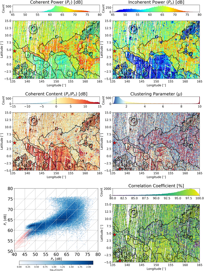
Figure 5. Maps and associated distributions of derived surface HK parameters. μ values higher than 10 are saturated as they cannot be discriminated with sufficient precision by our estimator. Black contours outline geologic unit boundaries (Tanaka et al. 2014). Red stars indicate Insight (+4°.5) and Curiosity (−4°.6) landing sites. The bottom left panel depicts the distribution of the measured surface echoes in the Pc − Pn space and also exhibits red contours outlining the distribution of background noise also shown in Figure 6.
Download figure:
Standard image High-resolution imageObservations. We observe that the relative dynamic range of the total signal spans about 30 dB, similar to what was observed by Grima et al. (2012) across a significant portion of the Martian surface, confirming that our selected case-study region is mostly representative of the power dynamic that could be encountered throughout the planet. Noticeably the full extent of this 30 dB dynamic range is mainly driven by Pn whereas the coherent signal Pc is due to geologic variations (i.e., not considering the background noise signal as determined below) and only spans ∼15 dB. The total radiometric range could be artificially reduced by the RSR-induced bias highlighted in our sensitivity analysis (Section 3.4) that is especially important for low coherent contents associated with high μ values. However, the facts that the derived μ values are mostly lower than 2 and that Grima et al. (2012) measured a similar dynamic range from the raw surface return (i.e., without resorting to the RSR methodology) suggest that this range underestimation is a minor effect.
Another important observation comes from the bulk of the measured coherent contents in decibels being positive, implying that the signal return at the antenna is often dominantly coherent. This is especially of interest for driving SHARAD data users toward an appropriate backscattering model for a surface properties inversion in a specific region. In particular, backscattering models for a dominantly coherent signal have a more tractable form and a reduced number of surface property unknowns than for a more balanced coherent–incoherent power location (e.g., Ulaby et al. 1981; Ogilvy 1991). Interestingly, rough terrains such as the MFF and some Noachian units exhibit a strong coherent content despite intuitively being expected to scatter the signal. In some cases, this coherency could be explained by the incoherent power fall-off being greater than for the coherent one (Haynes et al. 2018), so that the distance to the target naturally filters out the relative strength of the incoherent signal. In some other cases, a positive coherent content is simply the manifestation of the surface signal being so weak that our surface picker samples the random noise in a biased manner. The regions where these effects are dominant can be identified and discriminated as described in the following section.
Background noise. In locations where the surface signal is too dimmed to be reliably detected, the derived Pc and Pn components might be misinterpreted as proxies for the surface properties while they are in fact signatures of the background noise. To predict this effect and avoid geophysical interpretation pitfalls, we characterize the coherent signature of the background noise as seen by our surface picker. The purpose is not to characterize the noise itself, but rather to give insights on how the noise is rendered in the Pc − Pn space by the selective signal determination of our picker. For each radargram crossing, our region of interest, we run our surface picker into the first 100 earliest fast-time samples where the surface is usually absent. This is repeated 1000 times along track over equally spaced range lines. The obtained set of 1000 amplitudes is used to determine a single pair of Pc and Pn values per radargram through the RSR algorithm. The results reported in Figure 6 are within a range of relative power defined by Pc < 60 dB and Pn < 50 dB, and restricted into a narrow Pc /Pn ratio of 12 ± 0.5 dB.

Figure 6. Results obtained from our surface picker when run over SHARAD radargrams' background noise. Each point represents a Pc and Pn value associated to a single radargram. The whole cloud of points represents the range of RSR signature that should be expected in the absence of surface echo. Dashed diagonals are coherent content isolines.
Download figure:
Standard image High-resolution imageThanks to this range of values, one can identify the regions that correspond to background noise. The bottom left panel of Figure 5 represents the distribution of our samples in the 2D Pc − Pn space. The bottom left end of this distribution is split in two groups, both with Pn < 50 dB, but one with Pc > 60 dB while the other is coherently weaker than 60 dB. This latter group of points corresponds to the range of power for the background noise as outlined by the overlapping red contours. Interestingly, those two groups of points can be both geolocated within the MFF, indicating that the S/N of the surface echo there oscillates around the limit of detection for our surface picker. A closer look at the map of the incoherent power (Figure 5, upper right) shows that similar powers within the MFF tend to be arranged along track. It suggests that the S/N oscillations triggering the surface echo detection are driven by the conditions of acquisition (e.g., SA-HGA configuration, ionosphere attenuation) specific to each track.
4. Roughness Approximation
4.1. Coherent–Incoherent Growth
The behavior of the distribution in the 2D Pc − Pn space (bottom left panel of Figure 5) exhibits a noteworthy comma-like shape that we interpret in the context of signal growth with increasing surface roughness. This interpretation is detailed in the paragraph below through three types of regimes and illustrated by Figure 7. It will drive our logic for roughness approximation in the Section 4.2.

Figure 7. Sketches illustrating three typical regimes depicting the relative evolution of the coherent (Pc , green) and incoherent (Pn , red) power with increasing surface roughness for a nadir-looking radar. Three regimes illustrating milestones in the evolution of the signal powers are placed on the Pc − Pn distribution plot (left). Each regime is also illustrated in a surface backscattering radiation pattern (right). Dotted curves depict the evolution with increasing roughness of the relative strength of each type of power component in the normal direction. The area between the dashed curves is the coherent content.
Download figure:
Standard image High-resolution imageWhen the roughness increases over that of a flat surface (regime (1)) to a very rough surface with quasi-isotropic scattering properties (regime (3)), the coherent power diminishes until it eventually becomes undetectable. The coherent power lost thereby is progressively transferred into the pool of incoherent power, so that the incoherent power integrated over the half-space above the surface grows continuously with roughness. However, the incoherent power that is intercepted by the spacecraft at normal incidence does not exhibit a monotonic behavior. It first grows with roughness around the specular direction. But then, when the tilted surface elements reach a certain threshold depicted by regime 2, the growth of the incoherent power tends to be concentrated in off-normal directions, and counterintuitively, the incoherent power intercepted by the antenna around the normal then diminishes (Ulaby et al. 1981), going from regime (2) to regime (3), although the incoherent power integrated in the upper half-space increases. The coherent content provides another signature of this entire dynamic. It drops rapidly between regimes (1) and (2) since Pc and Pn evolve in an opposite manner. Then, the coherent content nearly stabilizes or even slightly increases, as both Pc and Pn shrink.
4.2. Analytic Relationships
The analytical relationships that bound the coherent and incoherent energies to the physical properties of the surface can be given by backscattering models. In general, at a given altitude z from the surface, at normal incidence, without volume scattering and for a stationary and ergodic surface, those components can be written in the forms


where α is a calibration constant that can be adjusted so that Pc = 1 (or 0 dB loss) when the surface is a perfectly flat and conductive reflector (Fresnel coefficient r = 1). r2 is the Fresnel reflection coefficient that is a function of the surface permittivity such as follows:
L(z) is the relative geometric propagation loss with respect to a specular reflection. For a flat surface, L(z) = 1/(π
z)2 (Grima et al. 2012). The surface roughness properties are defined by the rms height (σh
) and correlation length (lc
). For a more intuitive interpretation, we will refer to the effective slope se
= σh
/lc
(Campbell & Garvin 1993; Shepard et al. 2001). It is equivalent to the rms slope for a surface profile with an exponential autocorrelation (Ogilvy 1991).  and
and  are functions describing losses due to roughness. These are both dependent on the backscattering model considered. From Equations (2) and (3), it follows that the coherent content is independent on the surface permittivity and is only a function of the two roughness parameters when the altitude is known:

4.3. Methodology
When the surface backscatter tends toward regime (1) in Figure 7, the coherent power is weakly affected by roughness and is mainly dependent on the surface permittivity through r2. Our study area encompasses the transition between regime (1) to regime (2) through a distinguishable nearly horizontal distribution of measurements on Figure 7. The surface backscatter tends toward regime (1) for  . We use this value as a reference for the surface echo strength reflected from a flat surface (σh
= 0) with a given, but unknown, reflection coefficient
. We use this value as a reference for the surface echo strength reflected from a flat surface (σh
= 0) with a given, but unknown, reflection coefficient  . A surface with the same r2 that is affected by roughness will lose coherent power with respect to
  by a factor
  . This allows to associate each Pc
measurements to a σh
value. To this end, we use the analytical relationship
. This allows to associate each Pc
measurements to a σh
value. To this end, we use the analytical relationship  , where k is the wavenumber, as it tends to be an ubiquitous relationship across standard backscattering models as a first-order approximation (e.g., Ulaby et al. 1981; Ogilvy 1991).
Each measurement is now associated to a coherent content Pc /Pn and an rms height σh . Then, both can be injected into Equation (5) to derive a correlation length, where ζ(σh , lc ) is evaluated from the simplified integral equation method (IEM) that is valid for a stationary surface with normally distributed heights, with rms slopes <0.3 (∼17°) and with k σh < 2 (i.e., σh < 4.8 m at SHARAD wavelength) (Fung & Chen 2010).
The approximation for the surface roughness parameters obtained from this methodology is shown through the red grid on Figure 8. We note that the distribution of measurements lie within the application limits of the simplified IEM (Section 4.2).

Figure 8. Measurement distribution in the 2D Pc
− Pn
space overlapped by approximation of surface roughness parameters as described in Section 4.3 (red grid). Note that  is set as a flat surface reference with σh
= 0.
is set as a flat surface reference with σh
= 0.
Download figure:
Standard image High-resolution image4.4. Effect of Varying Surface Dielectric Constant
This inversion method allows for the quantitative approximation of the surface roughness parameters at the radar wavelength scale, and without the support of a third-party data set. However, it requires the fundamental assumption that the reflection coefficient  (or similarly permittivity, ε0) of theflat-surface reference is the same for all the terrains investigated. When this is not the case, the bias (or accuracy) induced on the approximated roughness can be estimated, provided that reasonable assumptions can be made regarding the permittivity difference between the two terrains. Let
  be the relative difference between the Fresnel coefficient of the flat-surface reference and another considered terrain r2
i
. Remember that both Pc
and Pn
are equally proportional to r2 (Equations (2) and (3)). It follows that the true roughness of the considered terrain can be obtained by (1) locating the position of its measured
be the relative difference between the Fresnel coefficient of the flat-surface reference and another considered terrain r2
i
. Remember that both Pc
and Pn
are equally proportional to r2 (Equations (2) and (3)). It follows that the true roughness of the considered terrain can be obtained by (1) locating the position of its measured  pair on Figure 8; (2) sliding diagonally from their by an amount Δr2 in both the x- and y- directions (i.e., parallel to the coherent content isolines); (3) the roughness values given at this new location on the plot are the true ones and can be compared with the roughness obtained at the initial
  location to estimate the bias.
For example, let us consider a terrain with measured surface components of  dB. The approximated roughness from Figure 8 is σh
= 1.8 m and se
= 12. Let us now consider ε0 = 9 and εi
= 4. These permittivities correspond to typical end values for materials of igneous origins (Ulaby et al. 1981), which we assume to be covering most of the studied regions as a first approximation. Δr2 is then equal to +3.5 dB, and the derived roughness parameters corrected from Δr2 are σh
≈ 1.4 m and se
≈ 10. Therefore, the accuracy of the derived roughness grows with Δr2, but it remains limited, especially when the surface is already rough. For nonvolcanic materials like nearly clean H2
O ice, εi
= 3.1 (Grima et al. 2009),
dB. The approximated roughness from Figure 8 is σh
= 1.8 m and se
= 12. Let us now consider ε0 = 9 and εi
= 4. These permittivities correspond to typical end values for materials of igneous origins (Ulaby et al. 1981), which we assume to be covering most of the studied regions as a first approximation. Δr2 is then equal to +3.5 dB, and the derived roughness parameters corrected from Δr2 are σh
≈ 1.4 m and se
≈ 10. Therefore, the accuracy of the derived roughness grows with Δr2, but it remains limited, especially when the surface is already rough. For nonvolcanic materials like nearly clean H2
O ice, εi
= 3.1 (Grima et al. 2009),  with a reference volcanic terrain of ε0 = 9 is 5.2 dB. In that case, a new flat-surface reference over an icy terrain would certainly provide better accuracy. When the surface is very smooth, the roughness bias due to Δr2 grows faster and might require other approaches to better assess the surface properties, such as the inversion technique combining the small angle approximation with the assumption of large correlation length (Grima et al. 2012, 2014a).
The bias due to the relative ignorance of the permittivity difference, between the reference terrain and the studied terrain, has to be combined with the uncertainties on Pc and Pn if the coherent content is outside of the confident ranges defined in Section 3.4.
4.5. Results
The methodology described in Section 4.3 provides a pair of roughness parameters (σh , se ) for each measured pair of coherent and incoherent surface echo powers (Pc , Pn ). The results are mapped on the top row of Figure 9. The bottom row provides comparable parameters independently obtained from the MOLA, but with different inversion techniques and at larger horizontal scales than SHARAD (Kreslavsky & Head 2000; Neumann 2003). A detailed study of the relationship between the SHARAD-derived roughness with the depositional and erosional geologic processes particular to this region will be addressed in a follow-on study. Our aim here is to discuss the validity of the so-derived roughness parameters by comparison with MOLA products. This work can be seen as an extension to the discussion initiated by Grima et al. (2012, Section 3) on the comparison between SHARAD total reflectivity and MOLA roughness.
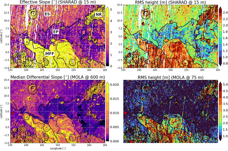
Figure 9. (Top) Effective slope (se ) and rms height (σh ) derived following our methodology applied to SHARAD surface reflectivity. (Bottom) Median differential slope at 600 m baseline (Kreslavsky & Head 2000) next to rms height at 75 m baseline, both derived from MOLA altimetry and MOLA pulse-width, respectively (Neumann 2003). Acronyms are shown to identify specific terrains discussed in the text: Elysium shield, Elysium plains, Medussa Fossae Formation and Noachian rise.
Download figure:
Standard image High-resolution imageSurface slopes. The MOLA median differential-slope product at 600 m scale (Figure 9, bottom left) is obtained from the median absolute values of the slopes measured at a 600 m horizontal baseline length from altimetry, but detrended from the regional slope measured at twice this scale (Kreslavsky & Head 2000). The removal of the regional topographic trend is responsible for the low, generally subdegree, median differential slope, making it hard to quantitatively compare with SHARAD roughness. However, the MOLA differential-slope product provides a good indicator outlining with fine sensitivity the spatial variations of intrinsic surface roughness that are really due to features at the baseline scale considered. The SHARAD-derived se at a 15 m baseline exhibits similar trends. The large outliers of the MFF (known to be rough at decameters scale; Mandt et al. 2008) and cratered NR appear both highly rough on SHARAD and MOLA slopes. More spatial variations can be distinguished within the MFF on the MOLA data set, while the SHARAD signal strength saturates at about se = 5°. This corresponds to the limit beyond which the signal strength reaches the background noise (Figure 5, bottom right), then becoming barely detectable. This behavior demonstrates that the upper limit of SHARAD sensitivity to roughness is controlled by its S/N capability to overcome extinction from strong surface scattering. Outside of those rough areas, many spatial nuances suggesting lava flow margins and/or structures in the smooth EP are mostly recovered in SHARAD-derived slopes similar to MOLA's, outlining small-scale variations in EP between 150°E and 155°E, for instance. The ES appear in both maps as terrains of intermediate roughness getting locally rougher within crater rims and ejecta.
Surface heights. The MOLA rms height (Figure 9, bottom right) is obtained from the relative spreading of the altimetric laser return after reflection onto the surface Neumann (2003). The result is a measure of vertical roughness at a horizontal baseline similar to the laser footprint diameter of ∼75 m, i.e., the smallest baseline at which roughness can be retrieved with global coverage so far. Theoretically, the linear additivity of the various sources of errors predicts that rms heights as low as 1 m can be resolved. Yet, the nuances of lava flows within EP are not recovered, while the transition from EP to ES is barely noticeable. The only terrains where inner variations are distinguishable are within the rougher MFF. By contrast, the SHARAD-derived rms heights at 15 m baseline still exhibit the subtle contrasts observed with the MOLA median differential slopes at 600 m baseline with the various geologic units considered. EP especially shows a large spectra of roughness from intermediate values of σh = 1.8–2 m gathered in a north–south band centered at 157° longitude that transitions abruptly eastward to a very smooth and narrow terrain with σh < 1 m, also seen on the MOLA median differential slopes. This latter terrain mostly contributes to the flat reference surface used in Section 4 to produce our roughness approximation grid. Its coherent content up to 15 dB is higher than that for the south polar layered deposits measured at 12 dB by Grima et al. (2012), and thus is one of the smoothest terrains observed on Mars.
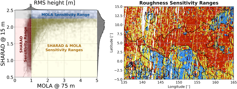
SHARAD-MOLA complementarity. The rms heights derived from SHARAD and MOLA are quantitatively compared in Figure 10 (left). Both data sets measured at different baselines are not expected to exhibit self-similarity (i.e., lying around the identity line) since bare planetary terrains are mostly observed to be self-affine (Shepard et al. 2001). However, Figure 10 displays specific behaviors worth mentioning. Two group of points can be distinguished that illustrate saturation effects related to both data products and their respective sensitivity range. A horizontal group of points aligned around the y coordinate 2.25 m outlines the detection limit beyond which the SHARAD surface return is lost into the background noise (Section 3.5.0.0). A vertical group of points mainly slightly below x-coordinate 1 m corresponds to measurements within ES and EP. These illustrate the lower-resolution limit of MOLA pulse-width measurements.
Figure 10. (Left) Scatter plot SHARAD-derived vs. MOLA pulse-length rms heights. Dashed line is the identity line. Colors indicate sensitivity ranges pertaining to each data set (σh < 2.25 m for SHARAD, σh >1 m for MOLA). Red, blue, and yellow are where SHARAD only, MOLA only, or both are within their sensitivity ranges, respectively. (Right) Mapping showing where the SHARAD and MOLA sensitivity are achieved. Color coding is the same as for the left figure.
Download figure:
Standard image High-resolution image
Those detection thresholds define ranges where both data sets are sensitive to roughness variation. Again, this range for SHARAD is <2.25 m, defining where the surface signal is not pure noise. It is >1 m for MOLA, a range where pulse-width variations are distinguishable from the pulse expected from a perfectly flat surface (Neumann 2003). Mapping the locations where those sensitivity ranges are achieved (Figure 10, right) provides highlights on how complementary the MOLA pulse-width and SHARAD roughness are when it comes to quantify relative rms heights at decametric scales. The roughest terrains (MFF and NR) are mainly within the detection limits of MOLA only (blue on Figure 10, right). By contrast, SHARAD provides the only measurement able to distinguish roughness variations throughout the smoothest terrains (red) like Elysium Planitia (Kreslavsky & Head 2000). Various transitional terrains between those two roughness behaviors can be characterized by both data sets (yellow). Thus, SHARAD complements MOLA at decametric scales since it can sense roughness variations over smooth terrains where the MOLA pulse-width technique is below its detection threshold. This can be informative for a finer quantitative comparison of smooth terrains to, for example, support the selection process of landing site candidates (e.g., Golombek et al. 2017) while small-scale measurements from MOLA pulse-width do not exhibit any contrast between sites. Note that two landing sites are covered by our study. SHARAD roughness of the most nearby measurements are about σh
= 1.5 m and se
= 13 for the Curiosity landing site, and σh
= 1.9 m and se
= 09 for the Insight landing site. MOLA provides σh
1.2 m and σh
< 1 m for Curiosity and Insight, respectively.
SHARAD-MOLA discrepancy. It is remarkable and counterintuitive that the rms heights are usually higher for SHARAD than for MOLA, while the SHARAD baseline length of 15 m is lower. Indeed, fractal laws predict that height variations of self-affine surfaces decrease with the horizontal scale at which they are measured (Shepard et al. 2001). We propose that this discrepancy is explained by the 2 orders of magnitude difference between the footprint size of SHARAD and that of MOLA. Indeed, although the SHARAD signal interacts with wavelength-sized (15 m) objects, the electromagnetic field received at the antenna is the coherent summation of all the fields scattered within the larger 5 km wide footprint. Hence, any large-scale trend of the surface, like kilometer-wide undulations, would increase the height range of the scatterers that contribute to the total phase of the wave front reaching the antenna, then increasing the approximated rms height. The effect of large-scale topography is much less pronounced for the MOLA pulse-length since the footprint contributing to the laser signal is only 70 m wide. To some extent, this effect is very similar to the MOLA median differential slopes giving much smaller values than those from altimetric roughness measurements not detrended from the regional slopes from Aharonson et al. (2001), Kreslavsky & Head (2000).
This hypothesis suggests that any quantitative multiscale comparison of radar-derived roughness should be wary of the footprint extent at which measurements are obtained in addition to the sounding wavelength. In addition, it also suggests that very small rms heights approximated from SHARAD (e.g., the submeter reference terrains within EP) are not only smooth but also necessarily extremely level across the 5 km footprint. These observations advocate for the use of fractal (self-affine) backscattering models whose surface roughness parameterization accounts, in essence, for variations at different scales (Franceschetti et al. 1999; Shepard & Campbell 1999; Campbell & Shepard 2003.
5. Conclusion
The surface echo strength recorded by radar sounders contains precious information about the surface roughness and near-surface structure at meter to decameter scales. However, their deconvolution and quantification from the surface-return strength is usually ambiguous and underconstrained. We apply the RSR methodology using homodyned K-statistics to the SHARAD data over a test region with a large radiometric spectra. The product provides several statistical parameters whose physical meaning in terms of heterogeneity population and distribution is described. The error estimation of those parameters in the presence of noise is negligible for coherent contents between −5 and 5 dB, while mostly limited and predictable if extended from −10 to 15 dB.
The coherent content is a strong relative indicator to drive the choice of an appropriate backscattering model for a further surface properties inversion. Most (but not all) of the covered terrains have a positive coherent content (suitable for quasi-specular models), including rough surfaces for which incoherent power is filtered out faster through differential geometric losses.
The measured Pc and Pn powers exhibit a very specific behavior that can be explained by the evolution of the surface scattering pattern with growing roughness. This finding enables us to identify smooth terrains that we use as flat references to estimate, from the IEM backscattering model, the roughness parameters of the entire studied area at, presumably, a 15 m horizontal baseline scale Fung (1994). This inversion technique preliminary requires the assumption of constant surface permittivity that necessarily introduces a bias in the retrieved roughness. However, this bias can be assessed if the permittivity difference between the studied terrains and the flat reference zone can be estimated or hypothesised. Any volume scattering would essentially add incoherent power to the signal. Therefore, following Figure 8, our neglecting of this diffusion effect would not affect the rms height approximation but will underestimate the effective slope when volume scattering is present. Also, the required assumption of homogeneous permittivity generates a quantifiable bias that is additive to the RSR error estimation (Section 4.4).
SHARAD roughness maps display subtle spatial variations similar to the MOLA median differential slope at 600 m scale. It also provides complementarity with greater sensitivity in smooth terrains where the MOLA pulse-width rms height at 75 m scale, the smallest baseline at which roughness can be retrieved with global coverage so far, is below its detection threshold. Large topographic variations within the SHARAD footprint could explain why SHARAD rms heights are usually greater than those derived from MOLA pulse-width, despite being sensed with a smaller theoretical baseline.
The properties of the smooth reference terrains located in Elysium Planitia suggest that these constitute the smoothest regions ever observed on Mars. Increasing the portfolio of smooth terrains identified by their flat Pc − Pn behavior, and with a large spectra of apparent permittivity, can also help approximate with better accuracy the decameter-scale roughness of terrains of various origins across the planet.
This study provides a wealth of radiometric observations and statistical descriptors to better relate radar reflectometry to geologic properties of planetary surfaces and near surfaces. These statistical descriptors can be used to discriminate and characterize terrains through the specific distribution of their structural heterogeneity (e.g., near-surface ices, lava flows, potential subsurface brines) at the radar wavelength scale. It also provides additional ways to complement landing site assessment with quantitative constraints on the surface roughness.
We would like to thank one anonymous reviewer and M. Kreslavsky for their insightful comments that greatly improved this manuscript. This work is supported by NASA under award No. 80NSS-C19K1492. It was also partially supported by the NASA Europa Clipper project and also by the G. Unger Vetlesen Foundation. Part of this research was carried out at the Jet Propulsion Laboratory, California Institute of Technology, under a contract with the National Aeronautics and Space Administration (80NM0018D0004). This is a UTIG publication 3880 and CPSH publication 0057. The radar surface properties derived in this study are available on the Texas Data Repository https://doi.org/10.18738/T8/GR884G.
Footnotes
- 7
- 8
All the applications, including error estimations, use the RSR processor v1.0.6 available at https://github.com/cgrima/rsr.