


Abstract
In a companion paper, we present the first spatially resolved polarized image of Sagittarius A* on event horizon scales, captured using the Event Horizon Telescope, a global very long baseline interferometric array operating at a wavelength of 1.3 mm. Here we interpret this image using both simple analytic models and numerical general relativistic magnetohydrodynamic (GRMHD) simulations. The large spatially resolved linear polarization fraction (24%–28%, peaking at ∼40%) is the most stringent constraint on parameter space, disfavoring models that are too Faraday depolarized. Similar to our studies of M87*, polarimetric constraints reinforce a preference for GRMHD models with dynamically important magnetic fields. Although the spiral morphology of the polarization pattern is known to constrain the spin and inclination angle, the time-variable rotation measure (RM) of Sgr A* (equivalent to ≈46° ± 12° rotation at 228 GHz) limits its present utility as a constraint. If we attribute the RM to internal Faraday rotation, then the motion of accreting material is inferred to be counterclockwise, contrary to inferences based on historical polarized flares, and no model satisfies all polarimetric and total intensity constraints. On the other hand, if we attribute the mean RM to an external Faraday screen, then the motion of accreting material is inferred to be clockwise, and one model passes all applied total intensity and polarimetric constraints: a model with strong magnetic fields, a spin parameter of 0.94, and an inclination of 150°. We discuss how future 345 GHz and dynamical imaging will mitigate our present uncertainties and provide additional constraints on the black hole and its accretion flow.
Export citation and abstract BibTeX RIS

Original content from this work may be used under the terms of the Creative Commons Attribution 4.0 licence. Any further distribution of this work must maintain attribution to the author(s) and the title of the work, journal citation and DOI.
1. Introduction
Synchrotron emission from the plasma near supermassive black holes (BHs) provides a crucial source of insight into the physical processes that drive accretion and outflow in galactic cores. It is intrinsically polarized, and both linear polarization and circular polarization provide information about the emitting plasma's density, temperature, composition, and magnetic field. In the rest frame of the emitting fluid, the linear polarization direction is orthogonal to the local magnetic fields, so images of linear polarization capture the projected magnetic field structure perpendicular to the line of sight. Any magnetized plasma along the line of sight imparts additional polarimetric effects via Faraday rotation, which rotates the plane of linear polarization with a λ2 dependence, where λ is the observing wavelength, and Faraday conversion, which exchanges linear and circular polarization states. Finally, for emission near a BH, the polarization is subject to achromatic rotation from propagation in a curved spacetime.
Recently, the Event Horizon Telescope (EHT) Collaboration published images of the supermassive BH at the Galactic center, Sagittarius A* (Sgr A*; Event Horizon Telescope Collaboration et al. 2022a, 2022b, 2022c, 2022d, 2022e, 2022f, hereafter Papers I–VI). These images revealed a bright emission ring encircling a central brightness depression (the "apparent shadow"), consistent with the expected appearance of a Kerr BH with a mass M ≈ 4 × 10⁶
M⊙ that is only accreting a trickle of material relative to that captured at the Bondi radius in a radiatively inefficient manner (e.g., Hilbert 1917; Bardeen 1973; Luminet 1979; Jaroszynski & Kurpiewski 1997; Falcke et al. 2000). Comparisons of the EHT measurements with numerical simulations provide estimates of the mass accretion rate  and a luminosity that is L ≲ 1036 erg s−1 ∼ 10−9
LEdd (see, e.g., Paper V, and references therein). Here
and a luminosity that is L ≲ 1036 erg s−1 ∼ 10−9
LEdd (see, e.g., Paper V, and references therein). Here  is the Bondi mass accretion rate and LEdd ≡ 4π
GMc
mp
/σT is the Eddington luminosity, with G, c, mp
, and σT being the gravitational constant, speed of light, proton mass, and Thomson cross section, respectively. Previously, measurements of linearly polarized emission near Sgr A* gave strong evidence for this low accretion state (e.g., Agol 2000; Quataert & Gruzinov 2000). In addition, the emission ring morphology, including the lack of a pronounced brightness asymmetry in EHT images, favors a viewing angle in Sgr A* that is at a low to moderate inclination (≲50°) relative to the angular momentum of the inner accretion flow (see, e.g., Figure 9 in Paper V).
is the Bondi mass accretion rate and LEdd ≡ 4π
GMc
mp
/σT is the Eddington luminosity, with G, c, mp
, and σT being the gravitational constant, speed of light, proton mass, and Thomson cross section, respectively. Previously, measurements of linearly polarized emission near Sgr A* gave strong evidence for this low accretion state (e.g., Agol 2000; Quataert & Gruzinov 2000). In addition, the emission ring morphology, including the lack of a pronounced brightness asymmetry in EHT images, favors a viewing angle in Sgr A* that is at a low to moderate inclination (≲50°) relative to the angular momentum of the inner accretion flow (see, e.g., Figure 9 in Paper V).
Event Horizon Telescope Collaboration et al. (2024, hereafter Paper VII) reports the first polarized images of Sgr A*, using EHT observations at 230 GHz taken in 2017. These images show a prominent spiral polarization pattern in the emission ring that is temporally stable, strongly linearly polarized (≈25%), and dominated by azimuthally symmetric structure. Both the image-averaged polarization fraction (mnet ∼ 5%) and the resolved polarization fraction (〈∣m∣〉 ≈ 25%) are significantly higher in Sgr A* than in the EHT's observations of M87* (Event Horizon Telescope Collaboration et al. 2021a, hereafter M87* Paper VII). In M87*, this polarization pattern was explained by coherent and dynamically important magnetic fields, depolarized by Faraday effects (Event Horizon Telescope Collaboration et al. 2021b, hereafter M87* Paper VIII).
In this paper, we provide the theoretical modeling and interpretation to accompany Paper VII. In Section 2, we summarize the new polarimetric observational constraints on Sgr A*. In Section 3, we provide general arguments about what these constraints imply for Sgr A* through comparison with three simple models: one-zone physical models to evaluate the plasma properties, geometrical ring models to evaluate the degree of coherence in the polarized image, and semianalytic emission models to evaluate the interplay between spacetime and emission parameters in determining polarized image structure. In Section 4, we describe a large library of general relativistic magnetohydrodynamic (GRMHD) simulations for Sgr A*. In Section 5, we evaluate which of these GRMHD models are compatible with the observational constraints. In Section 6, we summarize our findings and describe the prospects for improved constraints from future observations of Sgr A*.
2. Summary of Polarimetric Observations
In Paper VII, static polarimetric images are constructed from the Sgr A* EHT data taken on 2017 April 6th and 7 between 226.1 and 230.1 GHz (see Section 2 of Paper VII for more details). For theoretical interpretation, we adopt eight observational constraints derived from images generated by the THEMIS and the m-ring reconstruction methods (note that "m" is the azimuthal/angular mode number here, not polarization fraction; see Johnson et al. 2020). Of the four methods included in Paper VII, these are the only methods that provide Bayesian posteriors, from which we compute 90% confidence intervals. These methods make drastically different assumptions and, in a sense, bracket the possible spatial and temporal variability. In brief, the m-ring method fits a ring model to each snapshot independently, but the allowed spatial variability is very limited by construction (m ≤ 2 for total intensity, m ≤ 3 for linear polarization, and m ≤ 2 for circular polarization). In contrast, Themis attempts to optimize a single static image most consistent with the full data over time, with a noise budget attributed to time variability. Despite the vast differences between these models, they recover key image quantities with similar accuracy in synthetic data tests and arrive at mostly consistent observables (Paper VII).
Throughout this work, the large and time-variable rotation measure (RM) of Sgr A* poses a significant systematic uncertainty. Defined as RM ≡ Δχ/Δλ2, where χ is the electric vector position angle (EVPA), the RM of Sgr A* may originate from Faraday rotation internal to the emitting region, an external screen, changes in the plasma probed as a function of optical depth, or a combination of these effects. Examining the polarized light curves for the same 2 days as our EHT observations, Wielgus et al. (2024) arrive at  . We reserve a lengthy discussion of the RM of Sgr A* in both observations and theory for Appendix C. In summary, the fraction of the RM that can be attributed to an external Faraday screen is currently unresolved. Thus, throughout this work we consider the recovered image statistics both with and without RM derotation. Derotating the image corresponds to an interpretation where the time-averaged RM is attributed to a relatively stable external Faraday screen, separate from our models, which can be corrected for. Refraining from doing so corresponds to an interpretation in which all of the RM is generated internally, within our models. Our GRMHD simulations can reproduce the intraday variability of the RM, but not its stability of sign (see Appendix C).
For each of these methods, eight observational constraints explored in this paper are computed, listed in Table 1. To generate these ranges, a large quantity of images consistent with the data were generated from each method's posterior distribution. We computed the relevant observables for each of these images and then inferred 90% confidence regions. The m-ring method does not provide independent values of vnet, which is fixed to the mean ALMA-inferred value for circular polarization analysis (see Paper VII). When combining the two methods for theoretical interpretation, we adopt the minimum and maximum of the union of both 90% confidence regions (see Figure 10 in Paper VII for a visualization).
Table 1. Polarimetric Constraints Derived from the Static Reconstruction of Sgr A*
| Observable | m-ring | Themis | Combined |
|---|---|---|---|
| mnet (%) | (2.0, 3.1) | (6.5, 7.3) | (2.0, 7.3) |
| vnet (%) | ⋯ | (−0.7, 0.12) | (−0.7, 0.12) |
| 〈∣m∣〉 (%) | (24, 28) | (26, 28) | (24, 28) |
| 〈∣v∣〉 (%) | (1.4, 1.8) | (2.7, 5.5) | (0.0, 5.5) |
| ∣β1∣ | (0.11, 0.14) | (0.10, 0.13) | (0.10, 0.14) |
| ∣β2∣ | (0.20, 0.24) | (0.14, 0.17) | (0.14, 0.24) |
| ∠β2 (deg) (as observed) | (125, 137) | (142, 159) | (125, 159) |
| ∠β2 (deg) (RM derotated) | (−168, −108) | (−151, −85) | (−168, −85) |
| ∣β2∣/∣β1∣ | (1.5, 2.1) | (1.1, 1.6) | (1.1, 2.1) |
Note. These two methods each provide posteriors, from which 90% confidence regions are quoted. As constraints on our models, we conservatively adopt the minimum and maximum of these 90% confidence regions from both of these methods combined (rightmost column), with the exception of 〈∣v∣〉, which is treated as an upper limit. Derotation assumes that the mean RM can be attributed to an external Faraday screen, for which a frequency of 228.1 GHz is adopted.
Download table as: ASCIITypeset image
Table 2. Summary of the Sgr A* GRMHD Simulation Library Used in This Work
| Setup | GRMHD | GRRT | a* | Mode | Γad | tfinal | rout | Resolution |
|---|---|---|---|---|---|---|---|---|
| Torus | KHARMA | ipole | 0, ±0.5, ±0.94 | MAD/SANE |

| 50,000 | 1000 | 288 × 128 × 128 |
| Torus | BHAC | RAPTOR | 0, ±0.5, ±0.94 | MAD/SANE |

| 30,000 | 3333 | 512 × 192 × 192 |
| Torus | H-AMR | ipole | 0, ±0.5, ±0.94 | MAD/SANE |

| 35,000 | 1000/200 | 348/240 × 192 × 192 |
Note. The last column is N1 × N2 × N3, with coordinate x1 monotonic in radius, x2 monotonic in colatitude θ, and x3 proportional to longitude ϕ. Times are given in units of tg and radii in units of rg . Different settings may be adopted for MAD models compared to SANE ones, as denoted by a /.
Download table as: ASCIITypeset image
The quantities mnet and vnet correspond to the net linear and circular polarization that would be inferred from a spatially unresolved measurement for the time-averaged image. These are given by

where ∑i denotes a summation over each pixel i. For the time-resolved light curves, which are distinct from the values inferred from our static image reconstructions, Wielgus et al. (2022b, 2024) find 2.6% < mnet < 11% and −2.1% < vnet < − 0.7%, respectively, where we quote the central 90% of the values observed during the same 2 days of observation. Interestingly, we find that the m-ring method arrives at much lower values of mnet than Themis, which may be attributable to temporal cancellations of fluctuating EVPA patterns.
The remainder of our constraints are structural quantities, beginning with 〈∣m∣〉 and 〈∣v∣〉, the image-averaged linear and circular polarization fraction. These are given by


Note that these quantities depend on the effective resolution of our images. Throughout this work we quote values from our simulations corresponding to 20 μas resolution to mimic EHT resolution. We treat the resolved circular polarization fraction 〈∣v∣〉 as an upper limit, and thus the combined range extends to 0 in Table 1. This is due to the fact that the circularly polarized images presented in Paper VII show structural differences that we attribute to noise (see also Event Horizon Telescope Collaboration et al. 2023, hereafter M87* Paper IX). Because of the absolute magnitude inherent to the definition of this quantity, it is biased high when the signal-to-noise ratio is too low.
Complex βm modes correspond to Fourier decompositions of the linear polarization structure, where m refers to the number of times that an EVPA tick rotates with azimuth (Palumbo et al. 2020). These coefficients are defined by


where ρ and φ correspond to polar coordinates in the image and P = Q + iU. The rotationally invariant mode, β2, has natural connections to what we believe are azimuthally symmetric disk/jet structures, in particular the magnetic field geometry. Its amplitude encodes the strength of this mode, while its phase encodes the pitch angle and handedness of EVPA ticks. We observe ∠β2 closer to ±180° than 0°, which corresponds to tick patterns that are more toroidal than radial.
When considering observational constraints without RM derotation, we simply adopt the range of ∠β2 as observed on the sky. When considering observational constraints with RM derotation, we derotate ∠β2 assuming that there is an external Faraday screen between us and the emitting region that we can characterize by the mean RM over time. Since ∠β2 depends on twice the EVPA, we therefore add −2〈RM〉λ2 to ∠β2, where 〈RM〉 is the mean RM observed on April 6 and 7. Therefore, the range on ∠β2 had been significantly shifted by the Faraday screen by  deg. Applying this derotation both shifts and broadens the constraint.
Mean images from the posterior distributions generated by each method are plotted in Figure 1. Two sets of linearly polarized images are shown, corresponding to images without and with derotation, respectively. Note that derotation reverses the handedness of the polarization spiral, which has important implications for the flow structure. In the first two rows, total intensity is shown in gray scale, with contours drawn at 25%, 50%, and 75% of the peak brightness. These same contours are repeated in the bottom row. In the top and middle rows, the colored ticks encode linear polarization, where the length scales with the total linearly polarized intensity and the color scales with the fractional polarization. The dashed white contours plot the linearly polarized intensity rather than the total intensity.

Figure 1. Polarized images of Sgr A* used for physical interpretation in this work. Two methods from Paper VII, snapshot m-ring and THEMIS, are included. Top and middle: total intensity is shown in gray scale, polarization ticks indicate the EVPA, the tick length is proportional to the linear polarization intensity magnitude, and color indicates fractional linear polarization. The dotted contour levels correspond to linearly polarized intensities of 25%, 50%, and 75% of the polarization peak. The solid contour levels indicate total intensity at 25%, 50%, and 75% of the peak brightness. The top row shows images without derotation, and the middle row shows images with a derotation of 46.0 deg to account for Faraday rotation. Bottom: total intensity is indicated in solid colored contours at 25%, 50%, and 75% of the peak brightness, and the Stokes  brightness is indicated in the diverging color map, with red/blue indicating a positive/negative sign.
Download figure:
Standard image High-resolution imageFinally, we also compute the simplest nonrotationally symmetric mode, β1, as a probe of polarization asymmetry. Again, ∣β1∣ encodes the strength of this mode, and we use ∣β2∣/∣β1∣ as a probe of rotational symmetry. Since there is no clear axis (such as the spin axis) to define ∠β1 = 0°, we do not study ∠β1. We also refrain from computing higher-order βm modes, which are more likely to be sensitive to smaller-scale noise fluctuations.
3. Analytic Models
As discussed in the previous section, the linearly polarized image of Sgr A* exhibits three salient features:
- 1.It has a large resolved polarization fraction of 24%–28%, with a peak of ∼40%, much higher than M87*.
- 2.The linear polarization structure is highly ordered.
- 3.The ordered structure exhibits a high degree of rotational symmetry, which appears to spiral inward with counterclockwise handedness after derotating by the apparent RM, or clockwise without derotating.
Before exploring more physically complete GRMHD models, we demonstrate that each of these features can be understood in the context of simple analytic models.
3.1. One-zone Modeling
We use the basic assumptions described in Paper V that Sgr A* is an accreting BH with extremely small Eddington ratio and follow M87* Paper VIII to include polarimetry. This polarized one-zone model validates the more complicated numerical models shown later in this paper and offers a natural explanation for the high polarization fraction of Sgr A* relative to M87*.
We model the accretion flow around Sgr A* as a uniform sphere of plasma with radius r = 5 rg , where rg = GM/c2, comparable to the observed size of Sgr A* at 230 GHz (Papers III and IV), with uniform magnetic field oriented at a fiducial 60° inclination relative to the line of sight. The outcomes of our one-zone model depend only weakly on the field orientation. Note that the plasma velocity and the gravitational redshift are neglected.
In Paper V, we assumed that the plasma is optically thin, the ion−electron temperature ratio is 3, the ions are subvirial by a factor of 3, and plasma β ≡ Pgas/Pmag = 1. Adopting the observational flux constraint Fν
= 2.4 Jy (Wielgus et al. 2022a), we obtained the self-consistent solution ne
≃ 106 cm−3 and B ≃ 29 G. Using this solution, we can estimate the strength of the Faraday rotation at 230 GHz with the optical depth to Faraday rotation  :
:

where ρV
is the Faraday rotation coefficient (e.g., Jones & Hardee 1979). In contrast, similar modeling arrived at  for M87* (M87* Paper VIII). The value inferred for Sgr A* suggests that the internal Faraday rotation may not be negligible (see also Wielgus et al. 2024), but it also may not necessarily lead to substantial depolarization.
By including optical depth effects and using the Dexter (2016) polarized synchrotron emission and transfer coefficients, we relax some assumptions, such as ion−electron temperature ratios and virial factor, and plot the allowed parameter space as in M87* Paper VIII. Specifically,
- 1.we relax the flux constraint to 2 Jy < Fν < 3 Jy to include the effect of variability; and
- 2.we require the same assumption that Sgr A* is optically thin, i.e., τ < 1.
The above requirements are marked by the gray and green regions in Figure 2, respectively. The magnetic field strengths are shown as red dotted contour lines, and the different panels assume different plasma β. In blue, we plot the contour corresponding to  , beyond which internal Faraday depolarization becomes increasingly important. Unlike for M87* (see Figure 2 of M87* Paper VIII), we find that the regions where the total flux and optically thin constraints are satisfied only occur in Faraday thin regions of parameter space. We note that this is compatible with multifrequency RM measurements that suggest
  (Wielgus et al. 2024). Again, this is enough to noticeably rotate the EVPA pattern, but not enough to cause substantial depolarization.
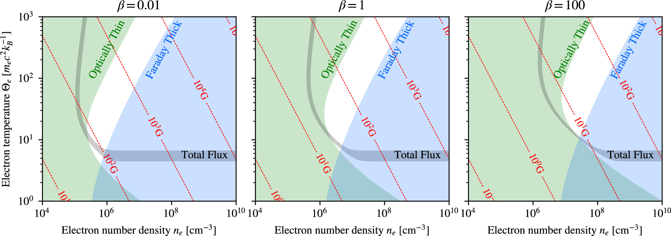
Figure 2. Allowed parameter space in electron number density (ne
) and dimensionless electron temperature (Θe
) for the one-zone model described in Section 3.1. The panels correspond to different assumed values of plasma β = Pgas/Pmag. We require that the total flux density 2 Jy < Fν
< 3 Jy (gray region) and optical depth τ < 1 (green region). Corresponding magnetic field strengths are shown as red dotted lines. In blue, we plot the Faraday thick region,  . Unlike for M87*, we find that the model is Faraday thin wherever there is intersection between our two constraints.
Download figure:
Standard image High-resolution imageIn summary, the total flux and optical depth constraints of Sgr A* naturally require small Faraday depths, which explains the large inferred values of 〈∣m∣〉.
3.2. Ordered Polarization: Ordered Fields
Because beam depolarization can only decrease the observed polarization fraction, measurements of the linear polarization at varying angular scales provide information about the degree of order in the underlying polarization. A priori, it could be possible that the the underlying magnetic field is significantly tangled on scales much smaller than the beam. However, the combination of unresolved (mnet ≈ 0.07) and EHT-resolved (〈∣m∣〉 ≈ 0.25) linear polarization measurements constrains the degree of order in the true, underlying polarization pattern on scales smaller than our beam size, disallowing significant spatially unresolved disorder.
As a simple toy model, we analyzed a thin, circular ring with polarization confined to two azimuthal Fourier modes, labeled with index ℓ. 155 First, we include a constant (ℓ = 0) mode that defines mnet. We fix the amplitude of this mode to be 0.07 to match unresolved observations of Sgr A*. Next, we add a second mode with varying index ℓ > 0 and an amplitude of 0.7, similar to the peak fractional polarization expected for synchrotron emission. By varying ℓ, we can crudely assess the allowed degree of coherence in the polarization of Sgr A*.
Figure 3 shows the resolved fractional polarization 〈∣m∣〉 at an angular resolution of 20 μas as a function of the secondary mode index ℓ. Both a perfectly ordered polarization field (ℓ = 0) and a highly disordered polarization field (ℓ ≫ 1) will have mnet ≈ 〈∣m∣〉. For the former, there is no beam depolarization; for the latter, the beam depolarization eliminates all small-scale polarized power, even at the resolution of the EHT. Hence, the high value of 〈∣m∣〉 relative to mnet that we observe is a powerful diagnostic of coherent polarized structure.

Figure 3. The combination of unresolved (mnet) and EHT-resolved (〈∣m∣〉) linear polarization measurements (at 20 μas resolution) constrains the degree of order in the underlying polarization image. In this schematic example, a polarized m-ring has a fixed net polarization, mnet ≡ 0.07 (denoted with the black dashed line), together with a single strongly polarized mode at higher order, ℓ, that controls the degree of disorder. For small values of ℓ, the resulting image is too ordered, with 〈∣m∣〉 exceeding our observed value for Sgr A* (denoted with the upper yellow band). For large values of m, the resulting image is too disordered, with beam depolarization eliminating the highly polarized image structure. In this example, the fields must be substantially ordered to be consistent with our observations of Sgr A*, with polarized structure that is coherent on scales of the ℓ ≈ 4 mode, corresponding to angular scales of θ ≈ 4θg ≈ 20 μas.
Download figure:
Standard image High-resolution imageAs expected, small values of ℓ produce resolved polarization fractions that are too high, while large values of ℓ produce resolved polarization fractions that are too low. Many effects that are not included in this toy model could further decrease the resolved fractional polarization—the amplitude of the small-scale polarization structure could be significantly less than the synchrotron maximum (e.g., from optical depth or Faraday depolarization), there could be a mix of more than two modes, and there could be radial polarization structure that causes beam depolarization. Hence, this example provides a conservative lower limit on the scale of coherent polarized structure. To be consistent with our measurements of Sgr A*, we require ℓ ≲ 4, corresponding to structure on angular scales of  . Here θg
= rg
/d, where d is the distance and 5θg
is the approximate radius of the emission ring in Sgr A*. Hence, even without detailed modeling, we anticipate that the underlying polarization in Sgr A* is highly ordered, with significant power on azimuthal scales of θ ≈ 4M or more. That is, the large resolved polarization fraction implies relative order of the magnetic field pattern on scales below the beam size.
. Here θg
= rg
/d, where d is the distance and 5θg
is the approximate radius of the emission ring in Sgr A*. Hence, even without detailed modeling, we anticipate that the underlying polarization in Sgr A* is highly ordered, with significant power on azimuthal scales of θ ≈ 4M or more. That is, the large resolved polarization fraction implies relative order of the magnetic field pattern on scales below the beam size.
3.3. Decoding the Polarization Morphology
Semianalytic models enable computationally inexpensive investigation of the effects of model parameters on images. For example, semianalytic models of radiatively inefficient accretion flows have been used for decades to gain tractable yet physically motivated insights into accretion flows (Bromley et al. 2001; Broderick et al. 2009, 2011, 2014, 2016; Pu et al. 2016; Pu & Broderick 2018; Vincent et al. 2022). Here we explore a very simple model, KerrBAM (or Kerr Bayesian Accretion Modeling), a semianalytic model for equatorial, axisymmetric synchrotron emission around a Kerr BH (Palumbo et al. 2022). This modeling framework carries out ray-tracing in a Kerr spacetime to produce a model image assuming an equatorial ring of emission with a specified fluid velocity, magnetic field geometry, and radial emission profile. Here we use this simple model to illustrate the effects of inclination and spin on polarized image structure.
As our starting point, we average 156 magnetic fields and velocity fields in three KHARMA GRMHD simulations (to be discussed in Section 4) in both time and azimuth. We specify a ring of emission centered at a radius of 6rg and use the values of the fluid velocity and magnetic field extracted from the GRMHD midplane at this radius. 157 To give the emission ring a realistically finite width, the emission is spread in a Gaussian spanning approximately 4rg –8rg , keeping the velocity and magnetic field vectors constant. With these values, KerrBAM is able to capture the effects of beaming, frame dragging, and lensing on the resultant image. Note that this model excludes the likely contribution of emission off the midplane (e.g., Falcke et al. 1993; Markoff et al. 2007).
For three different magnetically arrested disks (MADs) with spins of 0, +0.5, and +0.94, we plot several polarimetric quantities of interest (leftmost column) and their model images (subsequent columns) in Figure 4. Along with the polarimetric observables, we overlay our constraints in gray, where for ∠β2 the range without RM derotation is shown as a hatched region. Since this model places emission exactly at the midplane by construction, images produced at inclinations too close to 90° are misleading and therefore not included. The KerrBAM prescription does not include Faraday effects, only crudely modeling optical depth (in this case applying a midplane-normal crossing optical depth τ⊥ = 0.5 applied uniformly to  ,
,  , and
, and  ) and assuming a prespecified emission model confined to the midplane, so detailed agreement with the GRMHD models is neither expected nor achieved. Nevertheless, this model is useful for understanding several qualitative trends in our GRMHD library that are successfully reproduced.

Figure 4. Left column: image quantities determined from simplified analytic KerrBAM models evaluated using MAD GRMHD fluid velocities and magnetic fields of three spins. In this and subsequent figures, we plot our observational constraints as gray bands for reference, with the ∠β2 constraint prior to RM derotation shown as a hatched region. We use this model to understand key trends, but we caution that more physically complete GRMHD models are necessary for quantitative comparison. Right three columns: corresponding KerrBAM images evaluated at four example inclinations.
Download figure:
Standard image High-resolution imageFirst, the net polarization is minimized at low inclination, since the symmetry of the accretion flow causes cancellation of polarization in the integrated image. The amplitude of the rotationally invariant mode β2 is always high, due to the underlying azimuthal symmetry of the system. Meanwhile, the amplitude of ∣β1∣ is stronger at higher inclinations, as it is sensitive to asymmetries in the polarized image. Finally, we highlight the spin dependence of ∠β2, which this modeling demonstrates is driven by the evolution of the magnetic field and velocity structure in the GRMHD simulations due to frame dragging (see also Ricarte et al. 2022; Chael et al. 2023; Emami et al. 2023b). The a* = 0 model has ∠β2 ∼ −180°, corresponding to a very toroidal EVPA pattern and thus radial magnetic fields. Meanwhile, the higher spin models acquire −180 ≲ ∠β2 ≲ 0 owing to their more spiral EVPA structures. Interestingly, ∠β2 remains strikingly stable with inclination, although the overall image structure appears to evolve substantially by eye.
This exploration shows that some of the most salient qualitative features of the polarized image can be traced back to fundamental properties of the fluid and spacetime (magnetic field geometry and spin) without necessarily invoking more uncertain aspects of GRMHD models such as Faraday rotation, the electron-to-ion temperature ratio, and the electron distribution function. However, more physically complete calculations with GRMHD simulations that include these effects self-consistently are still necessary for quantitative comparison.
4. GRMHD Models
While semianalytic models provide qualitative insights and intuition about BH accretion flows, they do not enforce conservation laws or capture time-dependent phenomena such as turbulence and shocks that play a crucial role in determining the detailed system structure. Thus, we generate dynamical source models using numerical ideal GRMHD simulations. A fluid approximation would appear to conflict with the fact that the rate of Coulomb collisions is small, leading to mean free paths well exceeding the system size, implying that a collisionless kinetic treatment of the plasma may be necessary (Mahadevan & Quataert 1997). However, kinetic instabilities can produce small-scale inhomogeneities in the magnetic field that produce an effective collisionality through particle–wave interactions (Kunz et al. 2014; Riquelme et al. 2015; Sironi & Narayan 2015; Meyrand et al. 2019). We implicitly assume that radiative effects like cooling are not dynamically important for the fluid evolution. This assumption is well motivated given the low accretion rate of Sgr A*,  , for which the radiative cooling timescale is long compared to the accretion timescale (Dibi et al. 2012; Ryan et al. 2017; Chael et al. 2018; Porth et al. 2019; but see also Yoon et al. 2020).
In Paper V, to compare with total intensity EHT and multiwavelength constraints, we generated a suite of GRMHD-derived images sampling a range of initial conditions and parameterizations of the electron temperature and distribution function. We simplify our exploration in this work, limiting ourselves to simulations with untilted torus-like initial conditions, relativistic thermal electron distribution functions (eDFs) lacking nonthermal contributions, and electron temperatures prescribed via the Mościbrodzka et al. (2016) R − β prescription (see Equation (8) below). The properties of our GRMHD simulations are summarized in Table 2. Radiative transfer is integrated within a radius of 100rg , explicitly ignoring material in highly magnetized regions with σ ≡ b2/ρ > 1, within which mass density is artificially injected to keep the simulation stable. We briefly test the impact of our choices of outer integration radius, the σ cut, and the eDF in Appendices D–F, respectively. While departures from these assumptions are both interesting and physically justified, we defer a thorough investigation of these topics to future work.
Our GRMHD library samples a five-dimensional parameter space. The first parameter is the magnetic field state, either an MAD model (Bisnovatyi-Kogan & Ruzmaikin 1976; Igumenshchev et al. 2003; Narayan et al. 2003; Tchekhovskoy et al. 2011) or a standard and normal evolution (SANE) model (De Villiers et al. 2003; Gammie et al. 2003; Narayan et al. 2012; Sądowski et al. 2013). These describe models in which the magnetic flux threading the horizon for a given accretion rate has saturated and become dynamically important (MAD) or not (SANE). The second is the BH spin, which we denote as a* ∈ [ − 1, 1], where a negative sign indicates a retrograde disk with respect to the spin vector. Third is the inclination, which uniformly samples i ∈ [0°, 180°], instead of only i ∈ [0°, 90°] as probed in Paper V, because Faraday rotation and emission of circular polarization break the symmetry when polarization is considered. Our fourth parameter is Rhigh, which sets the asymptotic value of the ion-to-electron temperature ratio as plasma β → ∞ (Mościbrodzka et al. 2016). Specifically,

where Ti and Te are the ion and electron temperatures, respectively. While the potential importance of electron cooling for M87* motivated models with cooler electrons, Rlow = 10, here we only consider Rlow = 1 owing to the much smaller Eddington ratio of Sgr A*. Finally, our fifth parameter is the magnetic field polarity with respect to the angular momentum vector of the disk, either aligned or reversed, which affects the direction of Faraday rotation and the handedness of circularly polarized emission. This last degree of freedom only matters for polarized radiative transfer and was ignored in Paper V. We produce a library of images for each combination of these parameters, tabulated in Table 3.
Table 3. Summary of Parameters Sampled by Our GRMHD Libraries
| Parameter | Values |
|---|---|
| Magnetic field state | MAD, SANE |
| a* | −0.94, −0.5, 0.0, 0.5, 0.94 |
| i (deg) | 10, 30, 50, 70, 90, 110, 130, 150, 170 |
| Rhigh | 1, 10, 40, 160 |
| Magnetic field polarity | Aligned, Reversed |
Note. We coarsely sample a five-dimensional parameter space. For each combination of parameters and for each of the KHARMA and BHAC codes, we ray-trace the equivalent of 10 nights of observations.
Download table as: ASCIITypeset image
We retain the use of multiple codes to assess numerical systematic differences. For scoring, we generate libraries spanning 15,000tg (tg ≡ rg /c), equivalent to about 10 8 hr nights of observation for the parameter combinations listed in Table 3 using two code combinations: KHARMA 158 (Prather et al. 2021) + IPOLE 159 (Mościbrodzka & Gammie 2018) and BHAC 160 (Porth et al. 2017; Olivares et al. 2019) + RAPTOR 161 (Bronzwaer et al. 2018, 2020), where the first and second codes in each pair correspond to GRMHD and GRRT, respectively. As a further consistency check, a third set is generated with H-AMR 162 (Liska et al. 2022) + IPOLE for a subset of parameter space (only i ≤ 90°, aligned fields, and 5000tg ) that we do not use for scoring.
Each simulation is initialized with a torus of gas in constant angular momentum hydrodynamic equilibrium (Fishbone & Moncrief 1976). These tori are perturbed with a weak, poloidal magnetic field. The simulations vary in their initial radius of maximum pressure (from ∼15rg to 40rg ) and adiabatic index, Γad. Codes differ in their choice of Γad because Γad = 4/3 applies to a fluid of relativistic electrons and Γad = 5/3 applies to a fluid of nonrelativistic ions, but only one fluid is evolved in these models. Depending on the torus size and initial magnetic field configuration, the simulations develop into an MAD or SANE state (see, e.g., Wong et al. 2022).
In Figure 5, we plot a selection of time-averaged GRMHD snapshots from our library, blurred to EHT resolution using a Gaussian convolution kernel with an FWHM of 20 μas. In the left panel of each set we plot total intensity in gray scale and the resolved linear polarization as colored ticks. In the right panel of each set, we plot the circular polarization from blue to red with total intensity contours. Each panel is individually normalized such that the color maps span from 0 to the  on the left and
  on the right. Each of these models is an MAD a* = 0.94, Rhigh = 40 aligned field simulation, computed with different codes as indicated above.

Figure 5. Gallery of example time-averaged simulations in our library. Each panel displays a time-averaged and blurred (with a 20 μas FWHM Gaussian kernel) MAD a* = 0.94, Rhigh = 40 aligned models at three different inclinations. The first panel of each set displays total intensity and linear polarization, while the second panel of each set displays total intensity and circular polarization. Tick lengths scale the total polarized flux density in a given pixel, while their colors scale with the polarization fraction. H-AMR models are ray-traced only for a subset of models for comparison and are not used for scoring.
Download figure:
Standard image High-resolution imageThe codes exhibit agreement in terms of total intensity and polarized morphology but differ somewhat in the degree of polarization. As the inclination grows, the total intensity image becomes more asymmetric owing to Doppler beaming (e.g., Falcke et al. 2000; Medeiros et al. 2022; Paper V). The same holds true for the polarization, which is further affected by a Faraday depolarization gradient (see Appendix A.3). The magnetic field geometry as sampled by deflected light rays is encoded in the image of circular polarization. In particular, edge-on images in circular polarization exhibit sign inversions along both a horizontal and vertical axis due to flips in the line-of-sight magnetic field direction, and this signal disappears as the viewing angle decreases (Ricarte et al. 2021; Tsunetoe et al. 2021).
5. GRMHD Model Scoring
We introduce a novel methodology to score each of our GRMHD models using the eight polarimetric constraints in Table 1. Our new scoring scheme acts on time-averaged GRMHD images and attempts to accommodate variations between codes. Note that we only include quantities inferred from our polarimetric images in these constraints, but we will discuss comparisons with total intensity and multifrequency constraints derived in Paper V.
- 1.First, each model time series of images is split into 10 windows, each with 1500 M duration. Within each window, we produce a time-averaged image by averaging each of the Stokes parameters. Then, we blur the average image with a Gaussian kernel with an FWHM of 20 μas and compute each of the eight observables for scoring.
- 2.For each combination of parameters, we combine the values of the observables predicted by the KHARMA and BHAC codes. Since there are 10 windows and two sets of codes, this results in 20 different samples. From these values, we compute the 90% quantiles 163 of each observable to capture the time variability.
- 3.A model passes an individual observational constraint if there is overlap between its 90% quantile region and that of the observations. A model passes a set of observational constraints if it passes all of the constraints in the set simultaneously.
The most important differences compared to the scoring system utilized in Paper V are that this new system operates on time-averaged images and combines the results from multiple codes into a single theoretical range. We tested performing scoring using only one simulation set at a time. Since KHARMA model electron temperatures are assigned systematically hotter than those of the BHAC models (see Appendix H), KHARMA passes models with larger Rhigh. There is more disagreement between the codes for SANE models than for MAD models. The constraints with the most disagreement between the two codes are ∠β2, ∣β2∣/∣β1∣, and mnet, with the KHARMA simulations ruling out more SANE models than the BHAC simulations in each case.
Each of the observational constraints has known connections with the underlying physics. For brevity, we defer a pedagogical exploration of how each of our free parameters is imprinted onto the observables to Appendix A. We study how each individual constraint affects model selection in Appendix B. Here we summarize the highest-level scoring results, first excluding ∠β2 and then including ∠β2 either as observed or after performing RM derotation.
5.1. Constraints Independent of RM
In Figure 6, we plot a pass/fail table combining all polarimetric constraints, with the exception of ∠β2. These plots combine both polarities of the magnetic field, showing a pass as long as either polarity passes. These tables are slightly but not systematically different as a function of magnetic field polarity.
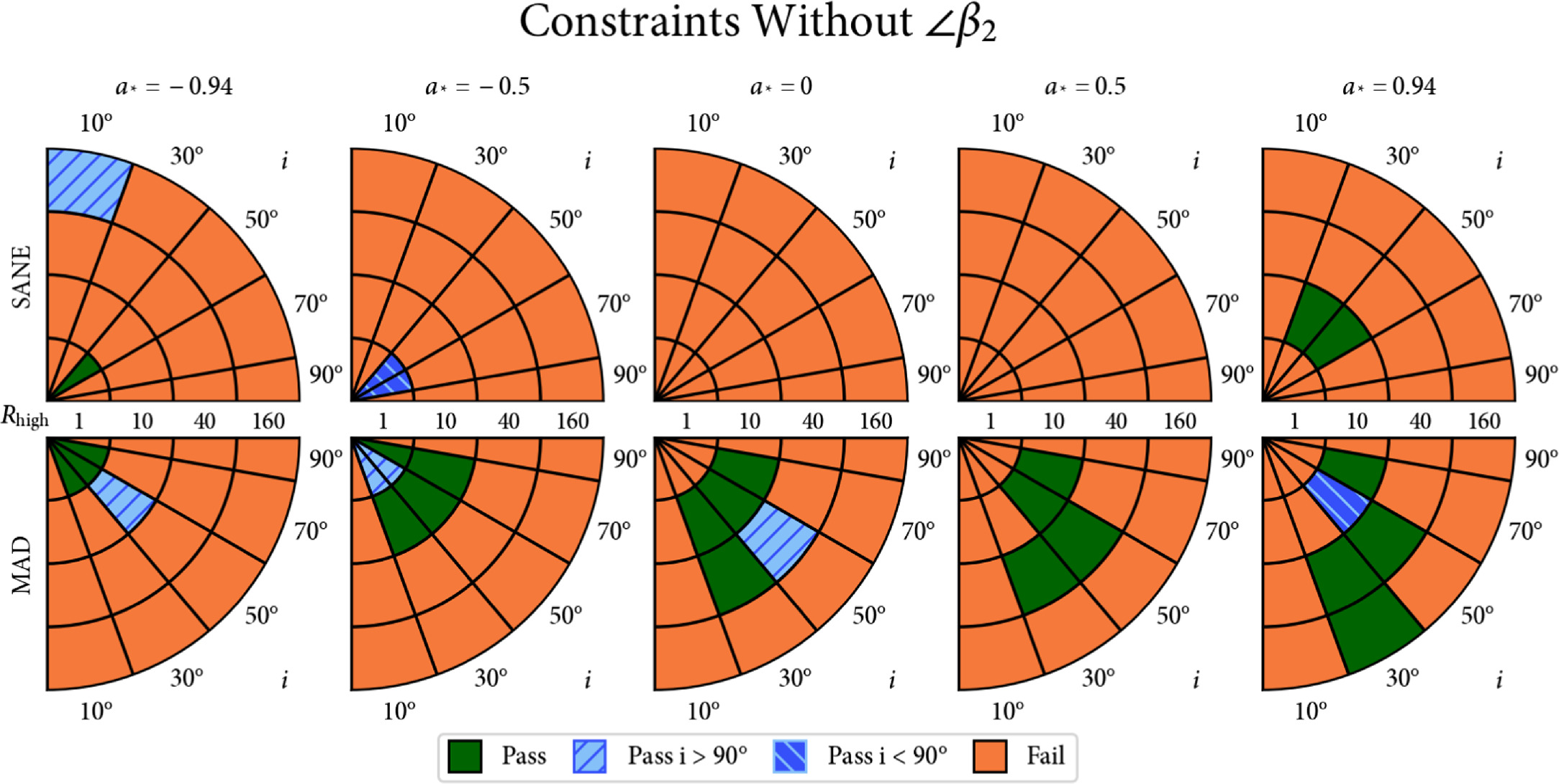
Figure 6. Combined polarimetric constraints on the GRMHD model library excluding ∠β2. Orange models fail, green models pass at both the given and its supplementary angle, and blue regions only pass with the given or supplementary angle as indicated. SANE models are plotted on the top half, and MAD models are plotted on the bottom half. Different columns correspond to different spins from −0.94 to 0.94. Within each wedge, the radial direction corresponds to Rhigh and the azimuthal direction corresponds to observer inclination.
Download figure:
Standard image High-resolution imageWe find that the tight constraint on 〈∣m∣〉 (24%–28%) is the most powerful, driving most of the trends shown in this figure. It is much more constraining on parameter space than mnet, for which a much larger range (2.0%–7.3%) is allowed. The ∣β2∣ constraint rules out a few additional typically edge-on models, but it does not provide too much more additional constraining power because 〈∣m∣〉 and ∣β2∣ are correlated. Without ∠β2, Figure 6 reveals no significant preference between i > 90° and i < 90° models.
While our total intensity constraints generally favored larger values of Rhigh (due largely to multiwavelength constraints; Paper V), our polarimetric constraints usually prefer more moderate values. This is because larger values of Rhigh usually lead to larger internal Faraday rotation depths (see Appendix A.4), which is the most important physical driver of depolarization in our models. However, an interesting trend with respect to spin allows one of the best-bet models of Paper V to continue to pass with Rhigh = 160. This is the MAD a* = 0.94, Rhigh = 160, i = 30°/150° model. MAD models with larger spin have smaller Faraday rotation depths (see Appendix H), allowing them to pass the 〈∣m∣〉 constraint for larger values of Rhigh. We refer readers to Appendix B for a more detailed breakdown of each constraint considered individually.
5.2. Constraints Including ∠β2 without RM Derotation
First, we discuss the ∠β2 constraint if RM derotation is not performed. It is possible that the RM may be attributed entirely to Faraday rotation captured within our simulation domain. GRMHD models are capable of producing the correct magnitude of RM from Faraday rotation on event horizon scales, but they tend to produce RM sign flips that are not consistent with decades of Sgr A* observations that produce negative values of the RM (Ricarte et al. 2020; M87* Paper VII; Wielgus et al. 2024). However, it is possible that this problem is related to the excess variability in our models identified in Paper V. We further discuss the uncertainties surrounding our interpretation of the RM in Appendix C.
If one attributes the RM entirely to internal Faraday rotation, then our constraint on ∠β2 spans the interval (125°, 160°). Adding this constraint to Figure 6 results in Figure 7. A selection for i < 90° arises because the handedness of the polarization spiral is opposite that of the magnetic field, which inherits the handedness of the inflowing and emitting gas (see Section 3.3 and Appendix A.3). This corresponds to counterclockwise motion, which disagrees with hot spot interpretations of polarized flares both in the near-IR (NIR; GRAVITY Collaboration et al. 2018, 2020a, 2020b) and in the submillimeter (Vos et al. 2022; Wielgus et al. 2022b). That is, consistency with clockwise motion would require −180° < ∠β2 < 0° if we assume that ∠β2 traces magnetic field lines with outgoing Poynting flux (Chael et al. 2023), which does not agree with the linearly polarized morphology as observed on the sky.

Figure 7. Same as Figure 6, but including the constraint on the phase of β2 without RM derotation. Only models with counterclockwise motion (i < 90°) pass. There is no model that passes all polarimetric and total intensity constraints utilized in Paper V.
Download figure:
Standard image High-resolution imageWithout RM derotation, no model can simultaneously pass all total intensity and polarimetric constraints. This is because the a* = 0.94 best-bet model of Paper V produces an EVPA pattern that is too radial (see Appendix A.2). All models that pass our polarization constraints in Figure 7 fail multiple constraints on the total intensity. In particular, all eight models shown in Figure 7 produce too much flux in the infrared to match observations, and all but the SANE model at a* = 0.94 overproduce the X-ray flux (Paper V). Both of these are serious failures, as both the IR and X-ray fluxes estimated by our models are lower limits owing to our lack of nonthermal electrons and small simulation domain relative to the X-ray-emitting area. Five of the models additionally fail to match the observed size and flux of the source at 86 GHz (Issaoun et al. 2019). All of these models also fail at least one total intensity structural constraint (m-ring and visibility amplitude morphology tests in Paper V). In conclusion, we cannot find a concordance model of Sgr A* without RM derotation.
5.3. Constraints Including ∠β2 with RM Derotation
Alternatively, in this section we interpret the mean RM as an external Faraday screen, motivating derotation. As discussed in Section 2, ∠β2 depends on twice the RM, for which a mean value of  has been obtained. This potentially results in a shift in ∠β2 of
  deg if this RM is interpreted as an external Faraday screen. In this picture, a relatively stable external screen explains the constant sign of RM that has been observed for decades (nevertheless with variation on the order of ∼105 rad m−2). Then, an additional component on event horizon scales, which is already included self-consistently in our models, explains the subhour time variability.
If one attributes the mean RM of a given day entirely to an external screen, then our constraint on ∠β2 spans (−168°, −85°). Adding this constraint to Figure 6 results in Figure 8. Performing this cut requires inclination angles >90°, corresponding to clockwise motion on the sky, which now agrees with the aforementioned models of polarized NIR and submillimeter flares.
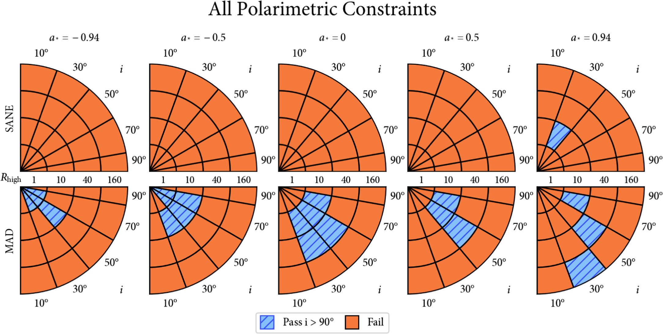
Figure 8. Same as Figure 6, but including the constraint on the phase of β2 with RM derotation. Only models with clockwise motion (i > 90°) pass. A best-bet model from Paper V passes all total intensity and polarimetric constraints: MAD a* = 0.94, Rhigh = 160, i = 150° aligned.
Download figure:
Standard image High-resolution imageWith RM derotation, one of the best-bet models from our total intensity analysis passes all applied total intensity and polarimetric constraints. This is the MAD a* = 0.94, Rhigh = 160, i = 150° aligned model. The second best-bet model from Paper V had a* = 0.5 and otherwise identical parameters. This second model passes all constraints except 〈∣m∣〉, which it underproduces by ∼3%. In order for the a* = 0.94 best-bet model to pass, at least 97% of the measured RM must arise from an external screen. Notably, the best-bet model fails if the smaller RM measured at 86 GHz a few days prior, (−2.14 ± 0.51) × 105 rad m−2 (Wielgus et al. 2024), is instead interpreted as the external screen.
In Figure 9, we visualize the best-bet model (BHAC shown) that survives with RM derotation. In the left two columns, we plot its full polarimetric image in the style of Figure 5. No blurring is applied in the leftmost column, and a 20 μas FWHM Gaussian kernel is convolved with the image in the second column to approximate EHT resolution. This model features a bright photon ring, and in our image without blurring, we omit total intensity contours from the circular polarization map to reveal a photon ring sign inversion (discussed in Mościbrodzka et al. 2021; Ricarte et al. 2021).
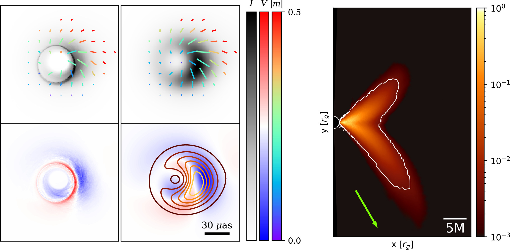
Figure 9. The best-bet model of Sgr A*: MAD a* = 0.94, Rhigh = 160, i = 150° aligned. In the left two columns, we plot its simulated image in the style of Figure 5. Images in the first column are unblurred, and images in the second column are blurred with a Gaussian with an FWHM of 20 μas, approximating EHT resolution. In the right panel, we provide a map of the emission in this model. The white contour encloses 90% of the total emission, the dashed white circle demarcates the horizon, and the green arrow indicates our viewing angle. While the emission peaks close to the BH in the midplane, a significant fraction of emission originates from a more diffuse region, including the jet sheath.
Download figure:
Standard image High-resolution imageOn the right, we produce a map of the density of the observed emission in the equivalent KHARMA simulation (using Kerr–Schild coordinates). The emission density map is normalized such that its peak value is unity, and it is visualized in logarithmic scale with 3 orders of magnitude in dynamic range. Our line of sight is indicated by the green arrow, and a white contour encloses 90% of the total emission. This reveals that while the emission is peaked at small radius near the disk midplane, a substantial fraction of the emission originates from a more diffuse jet funnel region. Computing an emission-weighted characteristic emission radius  , where
  is the emission density and x is the radius in cylindrical coordinates, we find
  . We note that our choices to include only thermal electron distribution functions and cut out regions with σ > 1 in this work minimize the potential contribution of a jet to the total emission (e.g., Figure 12 of Fromm et al. 2022). A significant jet component may be necessary to reproduce the flat spectral index at these frequencies (Falcke et al. 1993; Falcke & Markoff 2000; Mościbrodzka & Falcke 2013).
At a radius of 7.3rg
, we compute a mass-weighted average magnetic field strength of  , where the range quoted here corresponds to the 16th to 84th percentile values obtained in the time series. This value agrees reasonably well with the one-zone model discussed in Section 3.1, although we note that this value evolves substantially with radius, reaching
  at a radius of 4rg
and
at a radius of 4rg
and  at the horizon.
This model produces an outflow power of 4 × 1038 erg s−1 and has an accretion rate of 5 × 10⁻⁹ M⊙ yr−1. This model has a very large jet efficiency of approximately 150% powered by the Blandford & Znajek (1977) mechanism. Yet despite its efficiently, the jet's power is not high enough to expect global effects on the evolution of our Galaxy (e.g., Su et al. 2021).
6. Discussion and Conclusion
The first polarized image of Sgr A* on event horizon scales exhibits a high resolved polarization fraction of 24%–28% and an ordered, rotationally symmetric EVPA pattern. Through semianalytic arguments and comparisons to GRMHD simulations, we come to the following conclusions:
- 1.The large resolved polarization fraction implies that the magnetic field on event horizon scales cannot be very tangled on scales smaller than beam, nor can Faraday rotation add too much additional disorder to the EVPA structure. The disparity between the spatially resolved (24%–28%) and unresolved (2.0%–7.3%) linear polarization fractions can be attributed to cancellations due to the symmetric nature of the image.
- 2.Driven mostly by the spatially resolved polarization fraction, our constraints strongly favor MAD models over their SANE counterparts, as in M87* Paper VIII.
- 3.If we rely on internal Faraday rotation to produce the observed RM and do not perform derotation, then there is no model that passes all total intensity and polarimetric constraints.
- 4.On the other hand, if we assume that the RM can be attributed to an external screen and derotate the EVPA pattern, then we find one model that passes all applied total intensity and polarimetric constraints: MAD a* = 0.94, Rhigh = 160, i = 150° aligned.
While our ideal GRMHD simulations containing only thermal electron distributions have done remarkably well at reproducing many of the observed quantities of Sgr A*, they nevertheless have many known imperfections. Most of these models overestimate time variability, including the best-bet model (Paper V), and we caution that the values inferred from our best-bet model should not be interpreted as measurements. Known areas where these simulations can be improved include the following:
- 1.Initial Conditions : All of our simulations are initialized with tori that are either perfectly aligned or antialigned with the BH angular momentum axis. Simulations feeding the BH via stellar winds have different variability characteristics (Murchikova et al. 2022) and can self-consistently predict an external Faraday screen (Ressler et al. 2019, 2023). Tilted disk models (e.g., Fragile et al. 2007; Liska et al. 2018; Chatterjee et al. 2020) may lead to different Faraday rotation characteristics owing to their geometry at large radii.
- 2.Electron Thermodynamics : The Mościbrodzka et al. (2016) prescription that we adopt to set the electron temperature broadly captures the trends seen in kinetic simulations that explicitly model heating and cooling (e.g., Chael et al. 2018; Dexter et al. 2020; Mizuno et al. 2021; Dihingia et al. 2023) but does not reproduce them in much detail. More generally, a nonthermal contribution to the electron distribution function is believed to be necessary to reproduce the spectral energy distribution (Özel et al. 2000; Markoff et al. 2001; Davelaar et al. 2018) and is naturally predicted by particle-in-cell simulations (Kunz et al. 2016; Ball et al. 2018). Nonthermal electron distribution functions can have significant impacts on both total intensity and polarized properties (e.g., Markoff et al. 2001; Mao et al. 2017; Davelaar et al. 2018; Cruz-Osorio et al. 2022; Fromm et al. 2022; Paper V) and are a promising avenue to continue theoretical exploration.
- 3.Plasma Composition : Wong & Gammie (2022) demonstrate that models fed by helium rather than hydrogen may have substantially different emission morphologies, tending toward higher temperatures and lower densities and thus higher polarization fractions. Meanwhile, the presence of electron–positron pairs can significantly alter Faraday effects, leading to potential signatures in both linear and circular polarization that have not been fully explored (Anantua et al. 2020; Emami et al. 2021, 2023a; M87* Paper IX).
Several ongoing developments within the EHT will be impactful for testing our present interpretation, especially explorations in time and frequency. An effort is ongoing to produce dynamical movies of Sgr A*, despite the challenges of very sparse snapshot (u,v) coverage (Tiede et al. 2020; Farah et al. 2022; Levis et al. 2023). Measurements of the apparent angular velocity or potentially the motion of hot spots will provide additional constraints on spin and inclination (Wielgus et al. 2022b; Conroy et al. 2023). The dynamic reconstruction and geometric modeling of these data by Knollmüller et al. (2023) are consistent with the inferred inclination and clockwise motion of our best-bet model. On longer timescales (of years), it will be important to obtain averages of quantities such as ∠β2, which varies little in our models owing to its tight link with BH spin.
In the frequency domain, future EHT data sets will include 345 GHz data. The wavelength dependence of the scattering screen toward the Galactic center inhibits imaging of Sgr A* at lower frequencies below 86 GHz (Johnson et al. 2018; Issaoun et al. 2019, 2021). On its own, a 345 GHz polarized image would already strongly mitigate one of our largest systematic uncertainties, the RM; the total EVPA rotation would decrease by a factor of 2, as it is proportional to ν−2. These images will also have intrinsically higher resolution by a factor of 50%. Simultaneous dual-band observations could enable the production of RM maps, which would be our best tool for characterizing the Faraday screen and disambiguating our approach to derotation. If the RM truly originates from an external Faraday screen and the emission origin does not significantly change, then at 345 GHz we should observe a spatially uniform EVPA rotation of ∼20° clockwise relative to our 230 GHz image (roughly halfway between the top two rows in Figure 1). Meanwhile, RM due to internal Faraday rotation may exhibit more spatial variation and potentially sign flips owing to turbulence in the inner accretion flow (Ricarte et al. 2020).
Given the vastness of parameter and modeling space available to theoretical interpretation, we expect the polarized image of Sgr A* to continue to constrain models for many studies to come. This growing EHT data set will continue to challenge theoretical models and provide insights into the nature of BHs, accretion, and plasma physics.
Acknowledgments
The Event Horizon Telescope Collaboration thanks the following organizations and programs: the Academia Sinica; the Academy of Finland (projects 274477, 284495, 312496, 315721); the Agencia Nacional de Investigación y Desarrollo (ANID), Chile via NCN19_058 (TITANs), Fondecyt 1221421 and BASAL FB210003; the Alexander von Humboldt Stiftung; an Alfred P. Sloan Research Fellowship; Allegro, the European ALMA Regional Centre node in the Netherlands, the NL astronomy research network NOVA and the astronomy institutes of the University of Amsterdam, Leiden University, and Radboud University; the ALMA North America Development Fund; the Astrophysics and High Energy Physics program by MCIN (with funding from European Union NextGenerationEU, PRTR-C17I1); the Black Hole Initiative, which is funded by grants from the John Templeton Foundation (60477, 61497, 62286) and the Gordon and Betty Moore Foundation (Grant GBMF-8273)—although the opinions expressed in this work are those of the author and do not necessarily reflect the views of these Foundations; the Brinson Foundation; "la Caixa" Foundation (ID 100010434) through fellowship codes LCF/BQ/DI22/11940027 and LCF/BQ/DI22/11940030; Chandra DD7-18089X and TM6-17006X; the China Scholarship Council; the China Postdoctoral Science Foundation fellowships (2020M671266, 2022M712084); Consejo Nacional de Humanidades, Ciencia y Tecnología (CONAHCYT, Mexico, projects U0004-246083, U0004-259839, F0003-272050, M0037-279006, F0003-281692, 104497, 275201, 263356); the Colfuturo Scholarship; the Consejería de Economía, Conocimiento, Empresas y Universidad of the Junta de Andalucía (grant P18-FR-1769); the Consejo Superior de Investigaciones Científicas (grant 2019AEP112); the Delaney Family via the Delaney Family John A. Wheeler Chair at Perimeter Institute; Dirección General de Asuntos del Personal Académico-Universidad Nacional Autónoma de México (DGAPA-UNAM, projects IN112820 and IN108324); the Dutch Organization for Scientific Research (NWO) for the VICI award (grant 639.043.513), the grant OCENW.KLEIN.113, and the Dutch Black Hole Consortium (with project No. NWA 1292.19.202) of the research program the National Science Agenda; the Dutch National Supercomputers, Cartesius and Snellius (NWO grant 2021.013); the EACOA Fellowship awarded by the East Asia Core Observatories Association, which consists of the Academia Sinica Institute of Astronomy and Astrophysics, the National Astronomical Observatory of Japan, Center for Astronomical Mega-Science, Chinese Academy of Sciences, and the Korea Astronomy and Space Science Institute; the European Research Council (ERC) Synergy Grant "BlackHoleCam: Imaging the Event Horizon of Black Holes" (grant 610058); the European Union's Horizon 2020 research and innovation program under grant agreements RadioNet (No. 730562) and M2FINDERS (No. 101018682); the Horizon ERC Grants 2021 program under grant agreement No. 101040021; the European Research Council for advanced grant "JETSET: Launching, propagation and emission of relativistic jets from binary mergers and across mass scales" (grant No. 884631); the FAPESP (Fundação de Amparo á Pesquisa do Estado de São Paulo) under grant 2021/01183-8; the Fondo CAS-ANID folio CAS220010; the Generalitat Valenciana (grants APOSTD/2018/177 and ASFAE/2022/018) and GenT Program (project CIDEGENT/2018/021); the Gordon and Betty Moore Foundation (GBMF-3561, GBMF-5278, GBMF-10423); the Institute for Advanced Study; the Istituto Nazionale di Fisica Nucleare (INFN) sezione di Napoli, iniziative specifiche TEONGRAV; the International Max Planck Research School for Astronomy and Astrophysics at the Universities of Bonn and Cologne; DFG research grant "Jet physics on horizon scales and beyond" (grant No. 443220636); Joint Columbia/Flatiron Postdoctoral Fellowship (research at the Flatiron Institute is supported by the Simons Foundation); the Japan Ministry of Education, Culture, Sports, Science and Technology (MEXT; grant JPMXP1020200109); the Japan Society for the Promotion of Science (JSPS) Grant-in-Aid for JSPS Research Fellowship (JP17J08829); the Joint Institute for Computational Fundamental Science, Japan; the Key Research Program of Frontier Sciences, Chinese Academy of Sciences (CAS, grants QYZDJ-SSW-SLH057, QYZDJ-SSW-SYS008, ZDBS-LY-SLH011); the Leverhulme Trust Early Career Research Fellowship; the Max-Planck-Gesellschaft (MPG); the Max Planck Partner Group of the MPG and the CAS; the MEXT/JSPS KAKENHI (grants 18KK0090, JP21H01137, JP18H03721, JP18K13594, 18K03709, JP19K14761, 18H01245, 25120007, 23K03453); the MICINN Research Projects PID2019-108995GB-C22 and PID2022-140888NB-C22; the MIT International Science and Technology Initiatives (MISTI) Funds; the Ministry of Science and Technology (MOST) of Taiwan (103-2119-M-001-010-MY2, 105-2112-M-001-025-MY3, 105-2119-M-001-042, 106-2112-M-001-011, 106-2119-M-001-013, 106-2119-M-001-027, 106-2923-M-001-005, 107-2119-M-001-017, 107-2119-M-001-020, 107-2119-M-001-041, 107-2119-M-110-005, 107-2923-M-001-009, 108-2112-M-001-048, 108-2112-M-001-051, 108-2923-M-001-002, 109-2112-M-001-025, 109-2124-M-001-005, 109-2923-M-001-001, 110-2112-M-003-007-MY2, 110-2112-M-001-033, 110-2124-M-001-007, and 110-2923-M-001-001); the Ministry of Education (MoE) of Taiwan Yushan Young Scholar Program; the Physics Division, National Center for Theoretical Sciences of Taiwan; the National Aeronautics and Space Administration (NASA, Fermi Guest Investigator grant 80NSSC20K1567, NASA Astrophysics Theory Program grant 80NSSC20K0527, NASA NuSTAR award 80NSSC20K0645); NASA Hubble Fellowship grants HST-HF2-51431.001-A and HST-HF2-51482.001-A awarded by the Space Telescope Science Institute, which is operated by the Association of Universities for Research in Astronomy, Inc., for NASA, under contract NAS5-26555; the National Institute of Natural Sciences (NINS) of Japan; the National Key Research and Development Program of China (grant 2016YFA0400704, 2017YFA0402703, 2016YFA0400702); the National Science and Technology Council (NSTC, grants NSTC 111-2112-M-001-041, NSTC 111-2124-M-001-005, NSTC 112-2124-M-001-014); the US National Science Foundation (NSF, grants AST-0096454, AST-0352953, AST-0521233, AST-0705062, AST-0905844, AST-0922984, AST-1126433, OIA-1126433, AST-1140030, DGE-1144085, AST-1207704, AST-1207730, AST-1207752, MRI-1228509, OPP-1248097, AST-1310896, AST-1440254, AST-1555365, AST-1614868, AST-1615796, AST-1715061, AST-1716327, AST- 1726637,OISE-1743747, AST-1743747, AST-1816420, AST-1952099, AST-1935980, AST-2034306, AST-2205908, AST-2307887); NSF Astronomy and Astrophysics Postdoctoral Fellowship (AST-1903847); the Natural Science Foundation of China (grants 11650110427, 10625314, 11721303, 11725312, 11873028, 11933007, 11991052, 11991053, 12192220, 12192223, 12273022, 12325302, and 12303021); the Natural Sciences and Engineering Research Council of Canada (NSERC, including a Discovery Grant and the NSERC Alexander Graham Bell Canada Graduate Scholarships-Doctoral Program); the National Youth Thousand Talents Program of China; the National Research Foundation of Korea (the Global PhD Fellowship Grant: grants NRF-2015H1A2A1033752, the Korea Research Fellowship Program: NRF-2015H1D3A1066561, Brain Pool Program: 2019H1D3A1A01102564, Basic Research Support Grant 2019R1F1A1059721, 2021R1A6A3A01086420, 2022R1C1C1005255, 2022R1F1A1075115); Netherlands Research School for Astronomy (NOVA) Virtual Institute of Accretion (VIA) postdoctoral fellowships; NOIRLab, which is managed by the Association of Universities for Research in Astronomy (AURA) under a cooperative agreement with the National Science Foundation; Onsala Space Observatory (OSO) national infrastructure, for the provisioning of its facilities/observational support (OSO receives funding through the Swedish Research Council under grant 2017-00648); the Perimeter Institute for Theoretical Physics (research at Perimeter Institute is supported by the Government of Canada through the Department of Innovation, Science and Economic Development and by the Province of Ontario through the Ministry of Research, Innovation and Science); the Princeton Gravity Initiative; the Spanish Ministerio de Ciencia e Innovación (grants PGC2018-098915-B-C21, AYA2016-80889-P, PID2019-108995GB-C21, PID2020-117404GB-C21); the University of Pretoria for financial aid in the provision of the new Cluster Server nodes and SuperMicro (USA) for a SEEDING GRANT approved toward these nodes in 2020; the Shanghai Municipality orientation program of basic research for international scientists (grant No. 22JC1410600); the Shanghai Pilot Program for Basic Research, Chinese Academy of Science, Shanghai Branch (JCYJ-SHFY-2021-013); the State Agency for Research of the Spanish MCIU through the "Center of Excellence Severo Ochoa" award for the Instituto de Astrofísica de Andalucía (SEV-2017-0709); the Spanish Ministry for Science and Innovation grant CEX2021-001131-S funded by MCIN/AEI/10.13039/501100011033; the Spinoza Prize SPI 78-409; the South African Research Chairs Initiative, through the South African Radio Astronomy Observatory (SARAO, grant ID 77948), which is a facility of the National Research Foundation (NRF), an agency of the Department of Science and Innovation (DSI) of South Africa; the Toray Science Foundation; the Swedish Research Council (VR); the UK Science and Technology Facilities Council (grant No. ST/X508329/1); the US Department of Energy (USDOE) through the Los Alamos National Laboratory (operated by Triad National Security, LLC, for the National Nuclear Security Administration of the USDOE, contract 89233218CNA000001); and the YCAA Prize Postdoctoral Fellowship.
We thank the staff at the participating observatories, correlation centers, and institutions for their enthusiastic support. This paper makes use of the following ALMA data: ADS/JAO.ALMA#2016.1.01154.V. ALMA is a partnership of the European Southern Observatory (ESO; Europe, representing its member states), NSF, and National Institutes of Natural Sciences of Japan, together with National Research Council (Canada), Ministry of Science and Technology (MOST; Taiwan), Academia Sinica Institute of Astronomy and Astrophysics (ASIAA; Taiwan), and Korea Astronomy and Space Science Institute (KASI; Republic of Korea), in cooperation with the Republic of Chile. The Joint ALMA Observatory is operated by ESO, Associated Universities, Inc. (AUI)/NRAO, and the National Astronomical Observatory of Japan (NAOJ). The NRAO is a facility of the NSF operated under cooperative agreement by AUI. This research used resources of the Oak Ridge Leadership Computing Facility at the Oak Ridge National Laboratory, which is supported by the Office of Science of the U.S. Department of Energy under contract No. DE-AC05-00OR22725; the ASTROVIVES FEDER infrastructure, with project code IDIFEDER-2021-086; and the computing cluster of Shanghai VLBI correlator supported by the Special Fund for Astronomy from the Ministry of Finance in China. We also thank the Center for Computational Astrophysics, National Astronomical Observatory of Japan. This work was supported by FAPESP (Fundacao de Amparo a Pesquisa do Estado de Sao Paulo) under grant 2021/01183-8.
APEX is a collaboration between the Max-Planck-Institut für Radioastronomie (Germany), ESO, and the Onsala Space Observatory (Sweden). The SMA is a joint project between the SAO and ASIAA and is funded by the Smithsonian Institution and the Academia Sinica. The JCMT is operated by the East Asian Observatory on behalf of the NAOJ, ASIAA, and KASI, as well as the Ministry of Finance of China, Chinese Academy of Sciences, and the National Key Research and Development Program (No. 2017YFA0402700) of China and Natural Science Foundation of China grant 11873028. Additional funding support for the JCMT is provided by the Science and Technologies Facility Council (UK) and participating universities in the UK and Canada. The LMT is a project operated by the Instituto Nacional de Astrófisica, Óptica, y Electrónica (Mexico) and the University of Massachusetts at Amherst (USA). The IRAM 30 m telescope on Pico Veleta, Spain, is operated by IRAM and supported by CNRS (Centre National de la Recherche Scientifique, France), MPG (Max-Planck-Gesellschaft, Germany), and IGN (Instituto Geográfico Nacional, Spain). The SMT is operated by the Arizona Radio Observatory, a part of the Steward Observatory of the University of Arizona, with financial support of operations from the State of Arizona and financial support for instrumentation development from the NSF. Support for SPT participation in the EHT is provided by the National Science Foundation through award OPP-1852617 to the University of Chicago. Partial support is also provided by the Kavli Institute of Cosmological Physics at the University of Chicago. The SPT hydrogen maser was provided on loan from the GLT, courtesy of ASIAA.
This work used the Extreme Science and Engineering Discovery Environment (XSEDE), supported by NSF grant ACI-1548562, and CyVerse, supported by NSF grants DBI-0735191, DBI-1265383, and DBI-1743442. XSEDE Stampede2 resource at TACC was allocated through TG-AST170024 and TG-AST080026N. XSEDE JetStream resource at PTI and TACC was allocated through AST170028. This research is part of the Frontera computing project at the Texas Advanced Computing Center through the Frontera Large-Scale Community Partnerships allocation AST20023. Frontera is made possible by National Science Foundation award OAC-1818253. This research was done using services provided by the OSG Consortium (Pordes et al. 2007; Sfiligoi et al. 2009) supported by the National Science Foundation award Nos. 2030508 and 1836650. Additional work used ABACUS2.0, which is part of the eScience center at Southern Denmark University, and the Kultrun Astronomy Hybrid Cluster (projects Conicyt Programa de Astronomia Fondo Quimal QUIMAL170001, Conicyt PIA ACT172033, Fondecyt Iniciacion 11170268, Quimal 220002). Simulations were also performed on the SuperMUC cluster at the LRZ in Garching, on the LOEWE cluster in CSC in Frankfurt, on the HazelHen cluster at the HLRS in Stuttgart, and on the Pi2.0 and Siyuan Mark-I at Shanghai Jiao Tong University. The computer resources of the Finnish IT Center for Science (CSC) and the Finnish Computing Competence Infrastructure (FCCI) project are acknowledged. This research was enabled in part by support provided by Compute Ontario (http://computeontario.ca), Calcul Quebec (http://www.calculquebec.ca), and Compute Canada (http://www.computecanada.ca).
The EHTC has received generous donations of FPGA chips from Xilinx Inc., under the Xilinx University Program. The EHTC has benefited from technology shared under open-source license by the Collaboration for Astronomy Signal Processing and Electronics Research (CASPER). The EHT project is grateful to T4Science and Microsemi for their assistance with hydrogen masers. This research has made use of NASA's Astrophysics Data System. We gratefully acknowledge the support provided by the extended staff of the ALMA, from the inception of the ALMA Phasing Project through the observational campaigns of 2017 and 2018. We would like to thank A. Deller and W. Brisken for EHT-specific support with the use of DiFX. We thank Martin Shepherd for the addition of extra features in the Difmap software that were used for the CLEAN imaging results presented in this paper. We acknowledge the significance that Maunakea, where the SMA and JCMT EHT stations are located, has for the indigenous Hawaiian people.
Software: eht-imaging (Chael et al. 2016), Numpy (Harris et al. 2020), Scipy (Jones et al. 2001), Pandas (McKinney 2010), Astropy (The Astropy Collaboration et al 2013, 2018), Jupyter (Kluyver et al. 2016), Matplotlib (Hunter 2007), Themis (Broderick et al. 2020), ipole (Noble et al. 2007; Mościbrodzka & Gammie 2018), KHARMA (Prather et al. 2021), BHAC (Porth et al. 2017; Olivares et al. 2019), H-AMR (Liska et al. 2022), RAPTOR (Bronzwaer et al. 2018, 2020), KerrBAM (Palumbo et al. 2022).
Appendix A: Key Trends: Bridging Theory and Observations
Using our GRMHD models, we explore a five-dimensional parameter space, constrained by eight observable aspects of the polarized image that we believe are tied to the models in physically understood ways. Below, we highlight the most salient trends in our simulated image library to explain their physical origins. We focus on illustrative examples in this appendix, but we provide exhaustive distributions of observables calculated from our GRMHD models in Appendix H.
A.1. Magnetic Field State
By construction, SANE models have weaker magnetic fields near the horizon than their MAD counterparts at a given accretion rate. As a result, once the fluid is rescaled to reproduce the observed millimeter flux, SANE models usually have larger mass densities. This translates directly to a larger Faraday rotation depth, which is directly implicated for scrambling/depolarizing EHT model images (Mościbrodzka et al. 2017; Jiménez-Rosales & Dexter 2018; Ricarte et al. 2020; M87* Paper IX). Our SANE models are also colder (Paper V), which further increases the efficiency of Faraday rotation (Jones & O'Dell 1977; Quataert & Gruzinov 2000).
In Figure 10, we explore the differences between our MAD and SANE models with fixed a* = 0.5, Rhigh = 40, i = 50° and aligned fields. In the top panels, we plot the time-averaged KHARMA images in total intensity and linear polarization, blurred to a resolution of 20 μas. In the bottom panels, we compare differences in resolved linear and circular polarization fraction, Faraday rotation depth, and β2. In these and the following plots in this section, we display theoretical error ranges that are calculated based on differences between codes, time variability, and nearest neighbors in parameter space. The details of how these theoretical error bars are calculated are provided in Section 5.
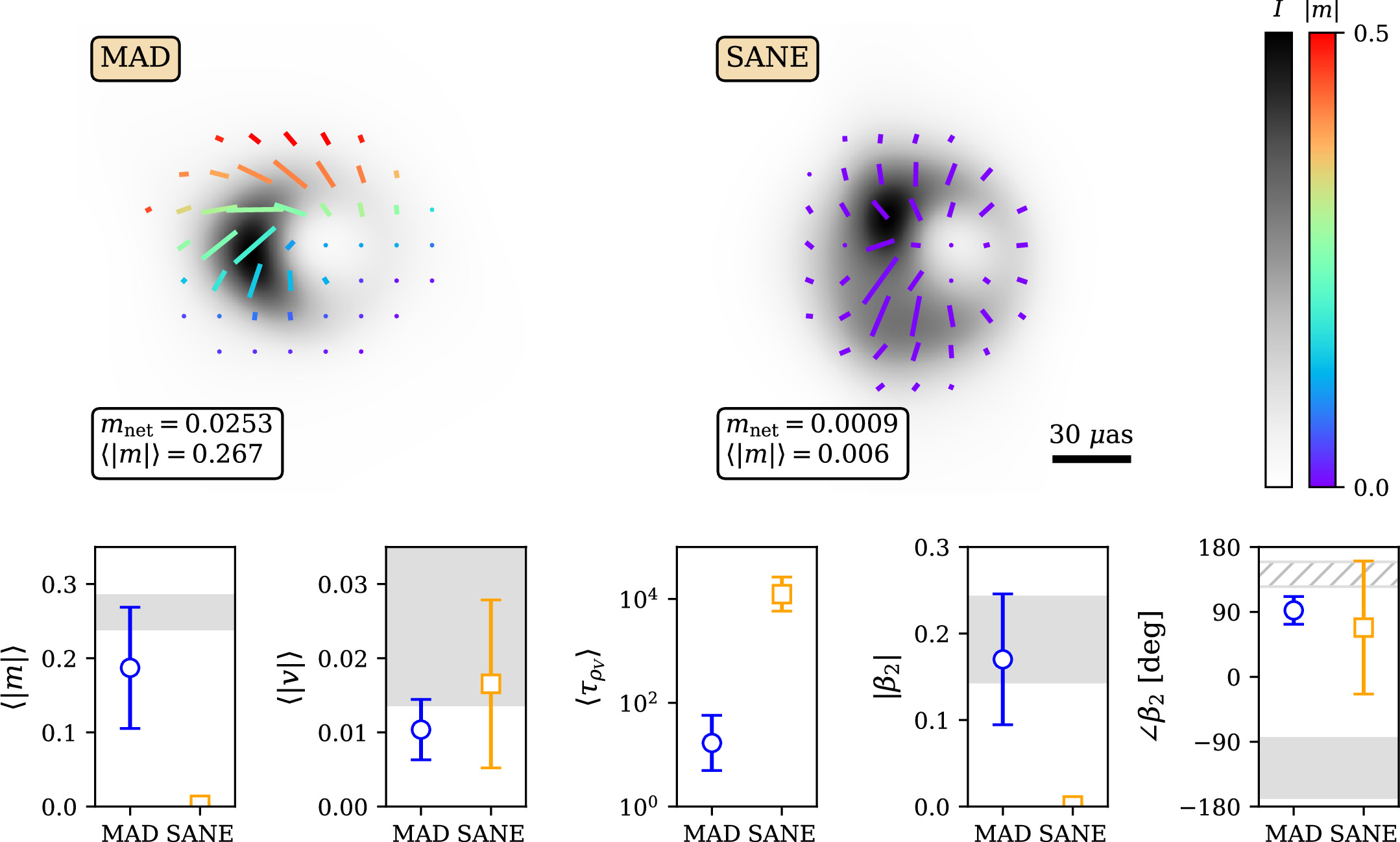
Figure 10. Comparison of the MAD and SANE a* = 0.5, Rhigh = 40, i = 50° aligned models (KHARMA images plotted). As in Figure 5, the lengths of the ticks scale with the polarized flux in each pixel, normalized for each model individually. A selection of polarimetric observables are shown with theoretical error bars, along with our observational constraints in gray. The constraint on ∠β2 prior to RM derotation is shown with a hatched band instead of a filled band. With other parameters held fixed, SANE models typically have lower resolved linear polarization owing to higher Faraday depths and can sometimes reach large values of circular polarization. Large Faraday depths in SANEs result in lower values of 〈∣m∣〉 and ∣β2∣.
Download figure:
Standard image High-resolution imageHere we see that the SANE model has much lower linear polarization fraction (〈∣m∣〉 and ∣β2∣), which can be attributed to a much larger Faraday depth ( ).
164
Much larger Faraday depths in SANE models than their equivalent MADs drive most of the differences between these two classes of models. SANE models can also produce larger circular polarization (〈∣v∣〉) owing to Faraday conversion (M87* Paper IX). Palumbo et al. (2020) showed that ∣β2∣ is a strong discriminant between MAD and SANE models of M87*. As expected, ∣β2∣ is significantly larger for the MAD model than for the SANE model. Interestingly, while SANE models of M87* usually exhibit ∠β2 ∼ 0, corresponding to radial EVPA patterns, the EVPA pattern in this SANE model acquires some twist owing to a tilted forward jet that we view in projection (top left).
).
164
Much larger Faraday depths in SANE models than their equivalent MADs drive most of the differences between these two classes of models. SANE models can also produce larger circular polarization (〈∣v∣〉) owing to Faraday conversion (M87* Paper IX). Palumbo et al. (2020) showed that ∣β2∣ is a strong discriminant between MAD and SANE models of M87*. As expected, ∣β2∣ is significantly larger for the MAD model than for the SANE model. Interestingly, while SANE models of M87* usually exhibit ∠β2 ∼ 0, corresponding to radial EVPA patterns, the EVPA pattern in this SANE model acquires some twist owing to a tilted forward jet that we view in projection (top left).
A.2. Spin
The BH spin is a particularly interesting quantity to constrain owing to implications for its cosmic assembly and feedback processes. A number of EHT-related studies have recently explored signatures of spin, and resolved linear polarization structure has been shown to be one of the most promising and accessible probes (Palumbo et al. 2020; Chael et al. 2023; Emami et al. 2023b; Qiu et al. 2023; Ricarte et al. 2023).
In Figure 11, we plot the phase and amplitude of β2 as a function of spin for the subset of the MAD Rhigh = 10, i = 30°/150° reversed models. The outer accretion disk rotates counterclockwise on the sky for i = 30° and clockwise on the sky for i = 150°, which is reflected by the sign of ∠β2 (or rather, the sign of its imaginary component). As discussed in Section 3.3, ∠β2 evolves with spin owing to frame dragging, which results in changes in the magnetic field and velocity structure (Palumbo et al. 2020; Event Horizon Telescope Collaboration et al. 2021b; Ricarte et al. 2022; Chael et al. 2023; Emami et al. 2023b; Qiu et al. 2023). The most highly spinning prograde models acquire a strong azimuthal magnetic field component, resulting in more radial EVPA patterns (∠β2 closer to 0°). Finally, ∣β2∣ is stronger for symmetric and ordered progrades than for their messier retrograde counterparts (see also Qiu et al. 2023).

Figure 11. Rotationally symmetric linear polarization structure as a function of spin, encapsulated in the phase and amplitude of β2. For this plot, MAD Rhigh = 10, i = 30°/150° reversed models are included, with either i = 30° in blue or i = 150° in red. Our observational constraints are shown as gray bands, and the constraint prior to RM derotation is shown as a hatched region. In this slice of parameter space, prograde models with spin values that are too large tend to produce polarization patterns that are too azimuthally symmetric and radially oriented compared to our observations.
Download figure:
Standard image High-resolution imageA.3. Inclination
The inclination of Sgr A* is of particular interest because its polarized flaring activity can be interpreted with a polarized hot spot model that favors a relatively face-on viewing angle (GRAVITY Collaboration et al. 2020a, 2020b; Wielgus et al. 2022b). In addition, it is of interest whether or not the accretion disk or BH angular momentum axes align with any structure in its environment.
Inclination is imprinted on the polarized image in a variety of ways, and we plot most of our polarimetric observables as a function of inclination in Figure 12. Here MAD a* = 0.94, Rhigh = 10 models are considered. These models produce rotationally symmetric images when viewed face-on, and thus cancellation leads to opposite behavior of mnet and 〈∣m∣〉, the latter of which decreases with inclination owing to Faraday depolarization. Intuitively, ∣β2∣, the amplitude of the rotationally invariant mode, is strongest for face-on viewing angles and weakest for edge-on viewing angles. Meanwhile, the asymmetric β1 mode has the largest amplitude for intermediate inclinations. The handedness of the linear polarization spiral is directly encoded in  , and thus we see that ∠β2 > 0° for i < 90° and ∠β2 < 0° for i > 90°. Finally, vnet is sensitive to whether the poloidal field is pointed toward us or away from us, but note that it is not perfectly antisymmetric about i = 90° owing to contributions from Faraday conversion (Ricarte et al. 2021).

Figure 12. A selection of polarimetric observables plotted as a function of inclination in a slice of our parameter space corresponding to MAD a* = 0.94, Rhigh = 10 reversed models. In very ordered models such as this one, symmetry and cancellation lead to the smallest net linear polarization fractions for face-on viewing angles at the same time that the resolved linear polarization fraction is highest. In this model, ∠β2 encodes the direction of motion, and vnet encodes the direction of the magnetic field with respect to the line of sight.
Download figure:
Standard image High-resolution imageA.4. Rhigh (Electron Temperature)
As described in Section 4, Rhigh sets the ratio of ion-to-electron temperature as plasma β → ∞ (Mościbrodzka et al. 2016). Increasing Rhigh while fixing all other parameters makes the electrons of a given model cooler and less efficient emitters. Thus, models with larger Rhigh tend to have larger values of  when rescaled to achieve the same target flux. As a result, increasing Rhigh indirectly increases the Faraday rotation depth (Mościbrodzka et al. 2017; Jiménez-Rosales & Dexter 2018; Ricarte et al. 2020; M87* Paper VIII). Increasing Rhigh also shifts emission away from the midplane and concentrates it toward the jet funnel region (Paper V; Wong et al. 2022). This effect is much weaker for MADs than for SANEs, since MAD models intrinsically have smaller plasma β on horizon scales.
In Figure 13, we plot time-averaged BHAC MAD a* = 0.5, i = 130° aligned field models as a function of Rhigh, as well as several of their linear polarization observables. Increasing Faraday depolarization explains the declines in 〈∣m∣〉 and ∣β2∣ with Rhigh. The polarization grows more asymmetric as Rhigh increases, because at this inclination the Faraday thick midplane is at the top half of the image. This, combined with increased Faraday rotation that slightly turns ticks clockwise, 165 leads to a shift in ∠β2. In addition, ∣β2∣/∣β1∣ decreases as the polarization grows more asymmetric.

Figure 13. Time-averaged images and a selection of polarimetric observables as a function of Rhigh, for the slice of our parameter space corresponding to MAD a* = 0.5, i = 130° aligned models (BHAC images plotted). In this slice of parameter space, Faraday rotation has a clear effect, since increasing Rhigh leads to smaller linear polarization fractions and correspondingly ∣β2∣. At this inclination, sight lines at the top of the image pass through the Faraday thick-disk midplane, increasing the polarization asymmetry as Rhigh increases, which is reflected in ∣β2∣/∣β1∣. Both line-of-sight Faraday rotation and changing emission regions lead to a trend in ∠β2.
Download figure:
Standard image High-resolution imageA.5. Magnetic Field Polarity
In ideal GRMHD, the equations governing the evolution of a magnetized fluid are invariant to a sign flip of the magnetic field direction. However, the equations of GRRT are not, leading to potential polarimetric signatures of the poloidal field direction. When performing radiative transfer, jV (intrinsic circular polarization of emitted radiation) and ρV (Faraday rotation) are each sensitive to the direction of the field with respect to the photon wavevector. The historically negative Stokes V of Sgr A* is suggestive of a magnetic field oriented away from us. However, M87* Paper IX discusses how flipping the magnetic field direction can have nontrivial effects on the circularly polarized image (beyond a simple sign flip) and noticeable effects on ∠β2 due to Faraday effects (see also Ricarte et al. 2021; Emami et al. 2023b).
In Figure 14, we highlight the differences between aligned and reversed field models for the time-averaged KHARMA MAD a* = 0.5, Rhigh = 160, i = 130° models. Each model is blurred with a 20 μas FWHM Gaussian beam shown in total intensity and linear polarization ticks on the left and circular polarization and total intensity contours on the right. We write ∠β2 and vnet for each model in the lower left corner, revealing significant and unpredictable differences, motivating independent ray-tracing for each magnetic field polarity. In linear polarization, the difference comes from reversing the direction that Faraday rotation shifts the EVPA pattern. The magnitude of this effect is larger than that reported in M87* Paper IX because M87* models are oriented almost completely face-on, viewed through an evacuated funnel (Ricarte et al. 2020). Models of Sgr A* can accumulate larger Faraday rotation depths as radiation passes through more of the disk at larger inclinations. In circular polarization, this particular model is mostly characterized by an overall sign flip, but this is not uniform across the image, leading to a small difference in vnet. This is because the coefficient of Faraday conversion, which exchanges linear and circular polarization, is invariant to a sign flip in the magnetic field direction.

Figure 14. Impact of reversing the polarity of the magnetic field on the time-averaged KHARMA MAD Rhigh = 160, a* = 0.5, i = 130° model. In radiative transfer, the handedness of Faraday rotation and intrinsic circularly polarized emission flip sign when the magnetic field flipped. This can lead to changes in the morphologies of both linearly and circularly polarized images.
Download figure:
Standard image High-resolution imageAppendix B: Impacts of Individual Observational Constraints
In Section 5, we included a limited selection of plots reflecting which of our models passed each of the polarimetric observational constraints on Sgr A*. Here we break down the impact of each constraint individually.
In Figure 15, we plot the impact of our 〈∣m∣〉 constraint, which we find is the most important for model selection. Compared to the other constraints, 〈∣m∣〉 is measured relatively precisely and the two methods agree very well. The Faraday rotation depth explains the trends in this figure (see Appendix H). More Faraday depolarization tends to occur if Rhigh is larger, if the inclination is larger, or if the model is SANE. Of the models that fail the 〈∣m∣〉 constraint, most are too depolarized, but some low-Rhigh, high-spin, face-on models are ruled out for predicting values of 〈∣m∣〉 that are too large. We find that 〈∣m∣〉 is much more constraining than mnet (Figure 16), which is measured much less precisely. Recall that mnet is substantially lower (and less consistent with the light curve) in the m-ring model than Themis. We find that if the higher and tighter mnet constraint from Themis had been adopted on its own, then this would have ruled out many face-on models (explained in Section 3.3 and Appendix A.3), including the a* = 0.94 best-bet model.

Figure 15. Individual impact of our 〈∣m∣〉 constraint on model selection. This tight constraint is our most informative, ruling out models that are either overly or insufficiently Faraday depolarized.
Download figure:
Standard image High-resolution image
Figure 16. Individual impact of our mnet constraint on model selection. This is less impactful than 〈∣m∣〉, mostly because the allowed range is much larger.
Download figure:
Standard image High-resolution imageOur circular polarization constraints are not very impactful. Our upper limit on 〈∣v∣〉 rules out no models (Figure 17), as all GRMHD models produce 〈∣v∣〉 lower than the upper limit (similar to M87* Paper IX). Our constraint on vnet is also not very impactful (Figure 18), but while not visible with our plotting scheme, it does rule out many retrograde models that have aligned fields. These models produce preferentially positive vnet, while decades of Sgr A* observations produce vnet < 0.
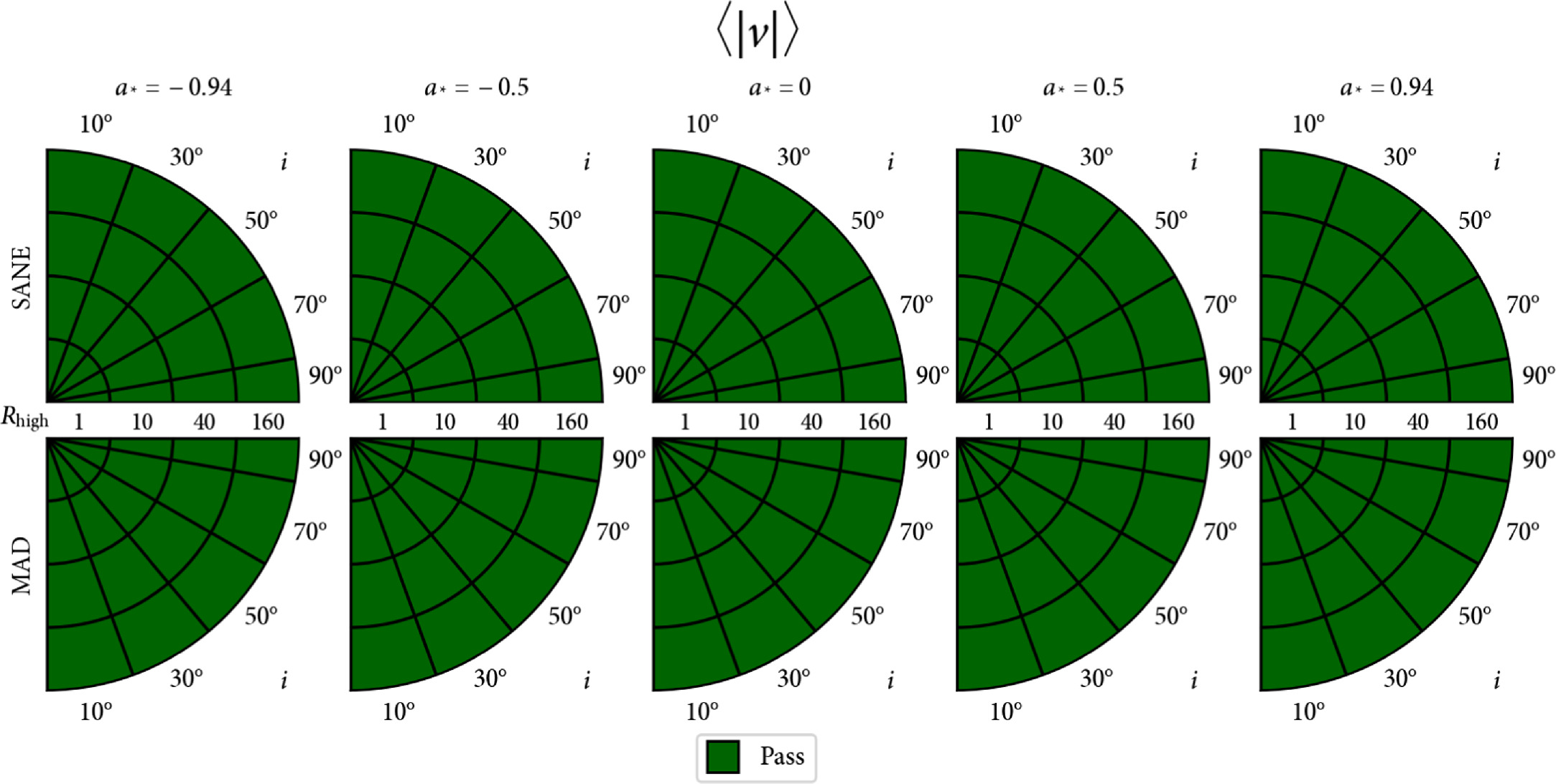
Figure 17. Individual impact of our 〈∣v∣〉 constraint on model selection, which is treated as an upper limit. All models naturally produce smaller resolved circular polarization fractions than this constraint.
Download figure:
Standard image High-resolution image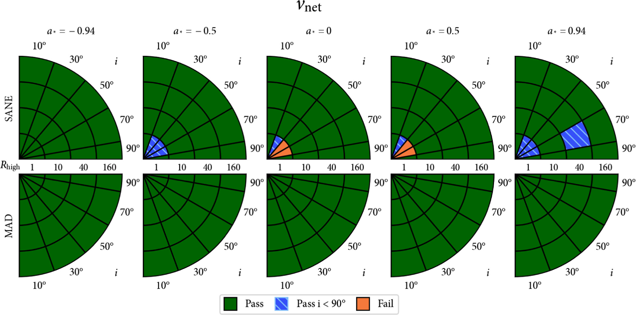
Figure 18. Individual impact of our vnet constraint on model selection. This is not very constraining, but it does rule out models whose distributions of vnet are skewed toward positive values.
Download figure:
Standard image High-resolution image
Figure 19. Individual impact of our ∣β1∣ constraint on model selection.
Download figure:
Standard image High-resolution imageOur constraints on ∣β1∣ (Figure 19), ∣β2∣ (Figure 20), and ∣β2∣/∣β1∣ (Figure 21) are impactful, but they are correlated with each other and 〈∣m∣〉. Compared to 〈∣m∣〉, ∣β2∣ additionally rules out some i = 90° models. The ratio ∣β2∣/∣β1∣ is not very constraining, as most models naturally produce ∣β2∣ > ∣β1∣, in agreement with the observations. While some methods in Paper VII produced ratios up to ∼5, which would have pushed our selection toward more face-on inclinations, the two methods retained in this paper produced more modest values. Interestingly, a few face-on models are ruled out for being too dominated by the rotationally symmetric mode.
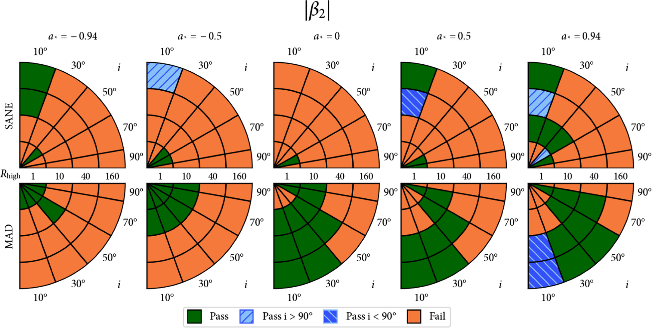
Figure 20. Individual impact of our ∣β2∣ constraint on model selection. This observable is correlated with 〈∣m∣〉 and behaves similarly.
Download figure:
Standard image High-resolution image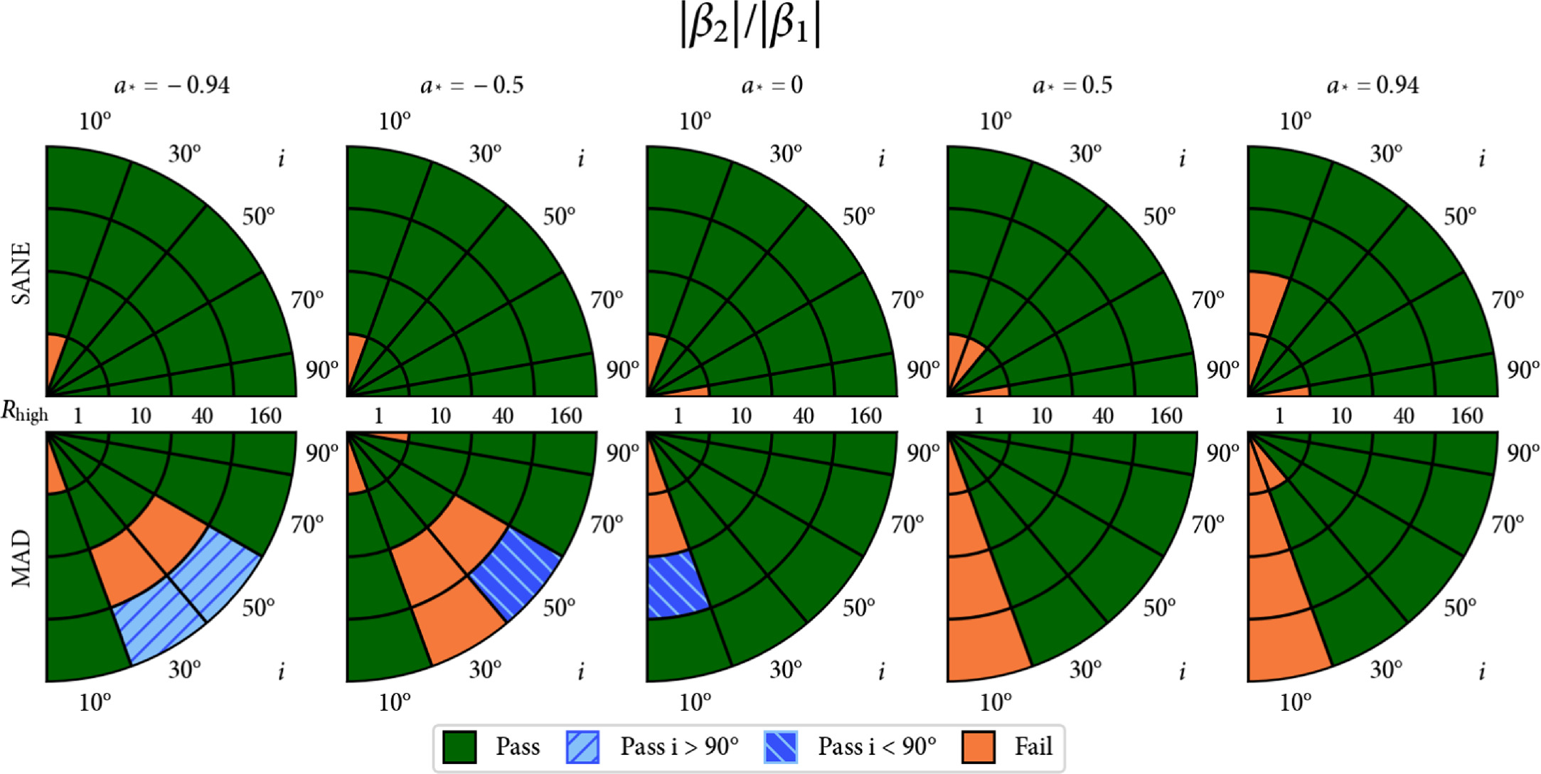
Figure 21. Individual impact of our ∣β2∣/∣β1∣ constraint on model selection. This only rules out a few face-on models that are too rotationally symmetric.
Download figure:
Standard image High-resolution imageFinally, we consider the effect of ∠β2 both with and without RM derotation in Figures 22 and 23, respectively. In either case, models with preferentially radial EVPA patterns are most likely to fail, such as face-on prograde MAD models (see Appendix A.2). With derotation, this constraint produces a preference for clockwise motion on the sky (i > 90°). Without derotation, the opposite is true, and more models fail outright since the constraint is tighter.
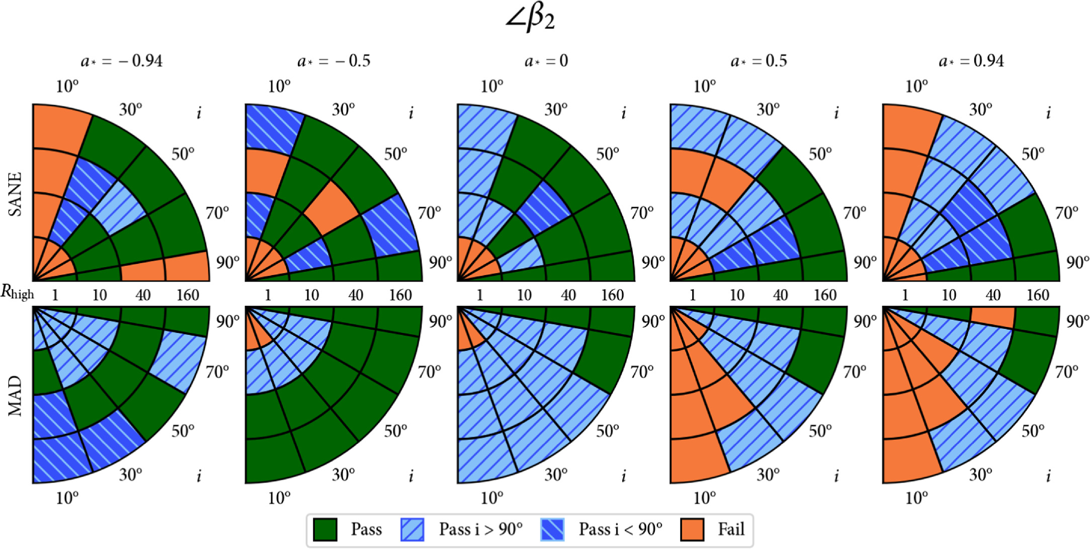
Figure 22. Individual impact of our ∠β2 constraint with RM derotation. This constraint produces a preference for i > 90°.
Download figure:
Standard image High-resolution image
Figure 23. Individual impact of our ∠β2 constraint without RM derotation. Compared to Figure 22, fewer models pass and there is now a preference for i < 90°.
Download figure:
Standard image High-resolution imageAppendix C: Rotation Measure
The RM of Sgr A* is a significant systematic uncertainty in our work, affecting our interpretation of ∠β2. The RM is defined as

where χ is the EVPA and λ is the wavelength. If the EVPA of the polarized emission does not intrinsically change with wavelength (due to optical depth), and the polarized emission is situated entirely behind a Faraday screen that is uniform relative to the size of the emitting region, then the RM is related to a path integral along the line of sight via
where ne
is the electron number density, B∣∣ is the local magnetic field parallel to the photon wavevector, and  , a factor causing lower efficiency as electrons become too relativistic (Jones & O'Dell 1977). If the two assumptions above are correct, then the "intrinsic" EVPA pattern can be easily recovered by derotating the EVPA by RMλ2.
Sgr A* has exhibited a constant sign of RM for decades (Bower et al. 2018), which supports the interpretation of a stable external Faraday screen. GRMHD simulations including RM from event horizon scales predict ubiquitous sign flips on subhour timescales that are not observed (Ricarte et al. 2020; Ressler et al. 2023; Wielgus et al. 2024). On the other hand, Sgr A* exhibits non- λ2 evolution of the EVPA when comparing the 86 GHz and 230 GHz bands. At 86 GHz, the RM on nearly simultaneous days to our observations is only −2 × 10⁵ rad m−2 compared to −5 × 10⁵ rad m−2 at 230 GHz (Wielgus et al. 2024). In addition to subhour time variability, this suggests that at least some of the RM must also come from internal Faraday rotation on event horizon scales.
Carefully predicting the RM directly for all of our GRMHD simulations would increase the computational cost by factors of a few (more than 2) with the software utilized in this work. This is because ray-tracing must be performed at different frequencies at nonuniform spacings to resolve potential phase wrapping and non-λ2 behavior of the EVPA. Nevertheless, we check the RM for a few snapshots of our models in Figure 24, where the RM is estimated by ray-tracing at 213, 215, 227, and 229 GHz (emulating observations) and then fitting for the slope RM = d χ/d λ2. MAD models are plotted in the top row, and SANE models are plotted in the bottom row. Three inclinations are shown: 30° in blue, 50° in orange, and 90° in gray. All models are at Rhigh = 40 and in an aligned field configuration. Note that these simulations only include material within 100rg , but ab initio simulations of the accretion of Sgr A* from stellar winds suggest that a steady Faraday screen could potentially be situated at even larger radii (Ressler et al. 2019, 2023).
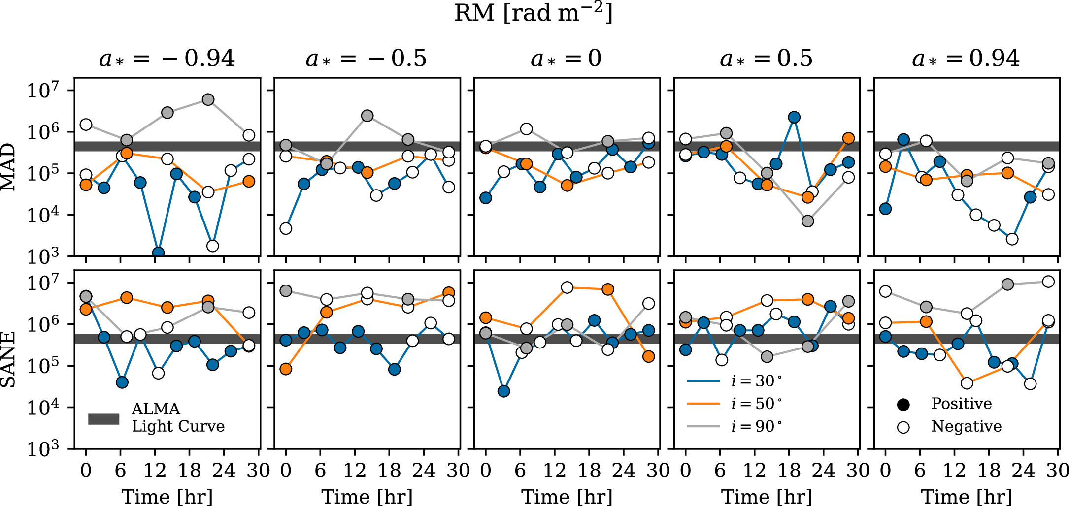
Figure 24. RM as a function of time for a selection of KHARMA model snapshots, each with Rhigh = 40 and aligned magnetic fields. Our models can roughly reproduce the observed magnitude of the RM but predict rapid sign flips (colored vs. white markers) that are not observed.
Download figure:
Standard image High-resolution imageWe find that most of our models naturally produce ∣RM∣ ∼ 105 rad m−2 at at least one point in time, in rough agreement with the observed value. The SANE models, as well as the MADs at 90°, tend toward larger values, similar to models of M87* (Ricarte et al. 2020). However, as in previous works, the RM flips sign in every model at least once. Interestingly, we find similar order-of-magnitude values of RM if Faraday rotation is explicitly switched off during ray-tracing (ρV = 0) in some of these models. This suggests that evolving emission origin as a function of frequency may contribute to the inferred RM and its variability.
Our findings in Figure 24 are broadly consistent with an interpretation wherein the rapid time variability of RM is caused by variability on event horizon scales, but the stability of sign is maintained by an external Faraday screen along the line of sight, motivating derotation of ∠β2. On the other hand, it may also be possible that all of the RM originates from event horizon scales, and our GRMHD models overpredict the variability in RM in the same way that they overpredict variability in total intensity (Paper V). To resolve this, 345 GHz imaging of Sgr A* will be critical; 345 GHz is less affected by Faraday rotation by a factor of (345/230)2 ≈ 2. In addition, RM maps produced via simultaneous multifrequency imaging will help determine the nature of the Faraday screen.
Appendix D: Impact of Outer Integration Radius
Although we are confident that most of the emission in our models originates close to the event horizon (r ≲ 10rg ), Faraday rotation can originate at much larger radius in our models, more so as the inclination increases (Dexter et al. 2020; Ricarte et al. 2020). This is especially problematic because material at these radii may not have had enough time in the simulation to reach equilibrium. This concern is more important for studies of Sgr A* than for M87* because we view M87* at an inclination of only 17° through an evacuated funnel.
We test the impact of the outer radiative transfer integration radius in Figure 25, where we ray-trace a few KHARMA snapshots at a variety of radii ranging from 30rg to 300rg . We focus on ∠β2, which should be directly affected by Faraday rotation on large scales. Inclinations of both 50° and 90° are considered, with Rhigh values of both 10 and 160. Fortunately, we find that ∠β2 appears to have converged for most of these models before 100rg , where we perform the ray-tracing in this paper. We find that the models that do exhibit substantial evolution with outer integration radius all produce 〈∣m∣〉 lower than observed. Note that SANE models at 90° inclinations with Rhigh = 160 are the most Faraday-thick models in our library. Models at i = 90 and/or high Rhigh appear to have the most evolution with respect to the integration radius. This is consistent with the expectation that higher inclinations and higher Rhigh values will increase the amount of Faraday rotation owing to more photons traveling through dense, cold regions in the GRMHD domain.

Figure 25. ∠β2 as a function of outer integration radius for a selection of KHARMA models. The GRRT in our work includes material at r ≤ 100rg , encoded by the gray band. Lines transition from thick to thin at the first radius at which ∣β2∣ < 0.05. For models with ∣β2∣ > 0.05, ∠β2 typically converges by r = 100rg .
Download figure:
Standard image High-resolution imageWhile ∠β2 appears to show evolution for some models, the other polarimetry metrics are well converged and show minimal change for all models across integration radius. However, although we have checked the GRRT step, recall that our GRMHD models are only converged within r ≲ 30rg owing to computational limitations. Exploration with simulations that are valid to larger radii that may produce an external Faraday screen self-consistently (e.g., Ressler et al. 2023) would be an interesting avenue for future analysis.
Appendix E: Impact of Cutting Jet Center ("σcut")
The polar funnel in the GRMHD simulations is filled with horizon-penetrating field lines and thought to contain plasma with orders of magnitude lower density than the accretion disk. By the same token, the funnel magnetization σ := B2/ρ is believed to be much larger than the magnetization in the disk. Since there are very few emitting particles in the funnel, its contribution to the overall image is expected to be negligible. In practice, to keep the numerical GRMHD evolution stable, σ is not allowed to assume realistic values but is instead capped at moderate values σ ≲ 50–100 by artificially injecting mass (e.g., Porth et al. 2019). Hence, we cannot trust the inflated mass density in this region. Assuming that emission in the σ ≫ 1 funnel should in reality be negligible, we follow the common practice and set all radiation transport coefficients to zero when the magnetization exceeds a critical value σcut = 1. This choice is only safe when no σ ≥ 1 regions form naturally in the disk and when the mixing of disk and funnel plasma at the jet wall is inefficient. In this case the gradient in magnetization is steep which means that whether we adopt σcut = 1 or, e.g., σcut = 25 does not affect the results. In reality, however, finite-resolution effects in the GRMHD simulations, resolved interchange instabilities, and potentially strong disk magnetization can cause a dependence on the adopted threshold value.
Using the BHAC/RAPTOR data, we have carried out spot checks with two "best-bet" models whereby we increase the threshold to σcut = 25: model 1 is MAD a* = 0, Rhigh = 40, i = 150° aligned, and model 2 is MAD a* = 0.94, Rhigh = 160, i = 30° aligned. In either case, the constraints change only by a few percent, e.g., in model 2 the average β2 phase changed from 63° to 66° and the average net polarization went down from 2.9% to 2.7%. In model 1, the change in average β2 phase is somewhat larger (going from −97° to −109°), but still small compared to the overall spread of the distributions. This shows that the results on polarized submillimeter emission are quite robust against change in the adopted value of the σcut and emission at or within the highly magnetized funnel does not dominate in the model.
Appendix F: Impact of Nonthermal Electrons
Throughout this work, we have considered only thermal eDFs when performing GRRT. Here we briefly explore the impact of nonthermal electrons in the polarimetric properties of one GRMHD model: MAD a* = 0, Rhigh = 40, i = 150° aligned. Two nonthermal prescriptions are explored:
- 1.
- 2.κ = 5: A κ distribution with a constant value of κ = 5 is applied globally (Davelaar et al. 2018).
We ray-trace 300 snapshots for each of these cases and compare with the thermal model snapshots. The accretion rate is kept fixed, but we find that the average flux density is 2.3 Jy for all cases. In Figure 26, we plot a selection of polarimetric quantities for these models. Each marker is placed at the median, and the error bars extend to the 16th and 84th percentiles. Overall, we find only subtle differences between these different eDF models. We find that 〈∣m∣〉 declines in the nonthermal eDF models, coincident with increases in the Faraday rotation depth (2.2, 4.2, and 6.3 for thermal, Variable κ, and κ = 5 models, respectively). Interestingly, vnet switches sign in the κ = 5 model, while ∠β2 varies only slightly, due to its link with the underlying field geometry. Overall, images with nonthermal eDFs will be useful to study in future work.

Figure 26. Comparison of thermal and nonthermal eDFs for MAD a* = 0, Rhigh = 40, i = 150° aligned models. Changes in the distributions of polarimetric quantities motivate future exploration in this area.
Download figure:
Standard image High-resolution imageAppendix G: An Interpolative Scoring Scheme
With our GRMHD models, we coarsely sample a five-dimensional parameter space. Here we investigate the possibility that this sparse sampling misses potentially passing models by performing scoring using expanded theoretical error bars. We conceptualize each combination of a*, Rhigh, and i as a volume in three-dimensional parameter space. For each neighbor in parameter space, if the 90% quantiles of the neighbor do not overlap, we linearly interpolate the lower and upper ranges of each observable to the midpoints of their nearest neighbors. This scheme helps mitigate sparse sampling but, as we discuss, may lead to false positives if observables evolve rapidly between adjacent models. In addition, this methodology fails to consider correlated evolution between observables.
In Figures 27 and 28, we show the results of our interpolative scoring scheme considering all polarimetric constraints without and with RM derotation, respectively. As expected, many more models pass in both cases. The preference for clockwise motion with derotation or counterclockwise motion without derotation is less dramatic with this scheme. Without derotation, both best-bet models still fail. With derotation, the second best-bet model from Paper V, MAD a* = 0.5, Rhigh = 160, i = 30°/150°, also passes in this scheme. Without interpolation, this model had only failed by producing too little 〈∣m∣〉.
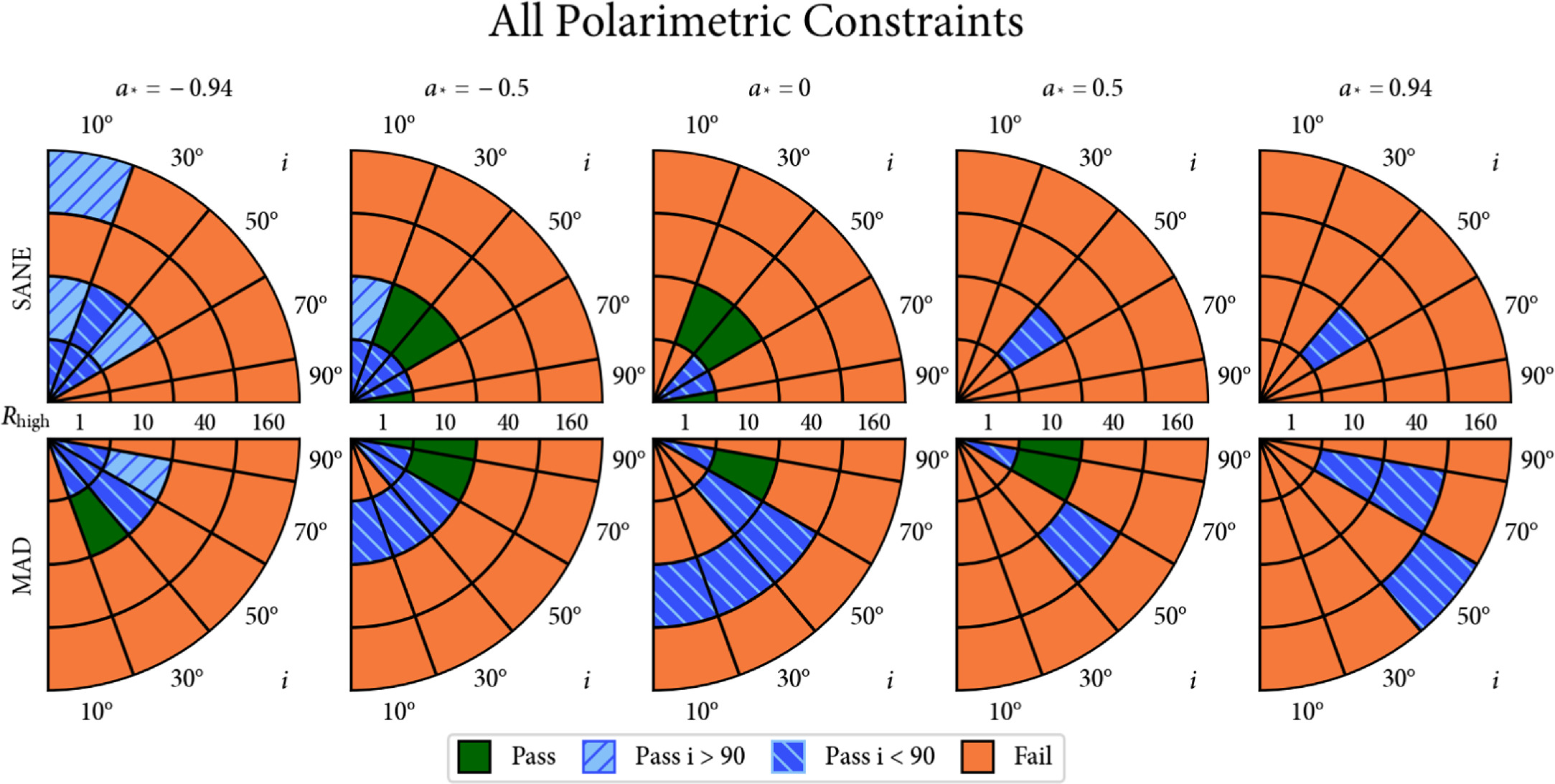
Download figure:
Standard image High-resolution image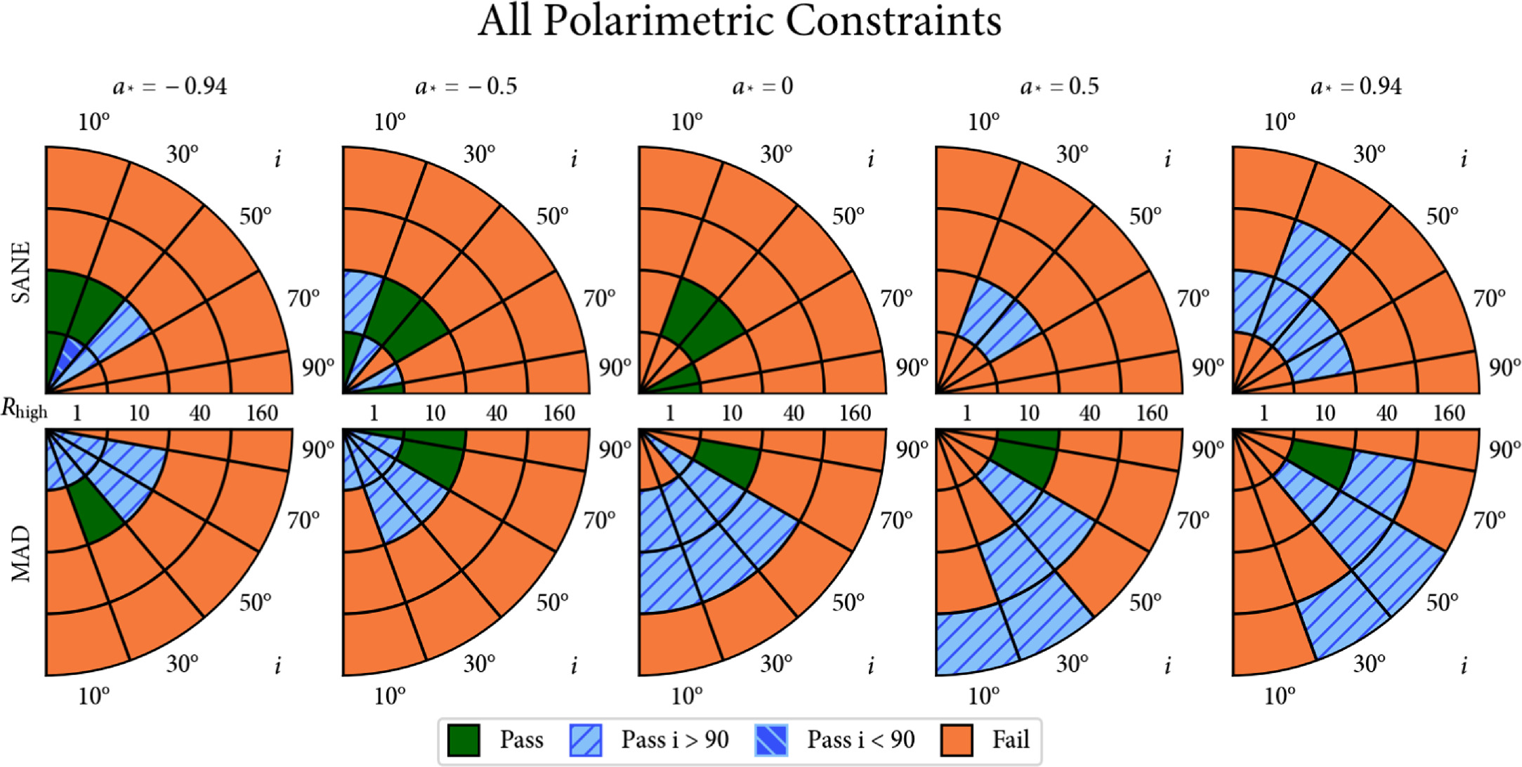
Download figure:
Standard image High-resolution imageThis interpolative scoring scheme does not produce as clear of a preference for MAD over SANE models. We find that this difference is driven by a shortcoming of this method: SANE models evolve very rapidly with Rhigh, especially between Rhigh = 1 and Rhigh = 10, leading to very large theoretical error bars. We explore one example in Figure 29, where a set of KHARMA SANE a* = − 0.5, i = 150° aligned field models are ray-traced at intermediate values of Rhigh ∈ {3, 5, 8}. Each of our eight polarimetric observables is plotted, and we better resolve the rapid evolution in these parameters with Rhigh. A noteworthy interaction occurs in our interpolation scheme with 〈∣m∣〉 and ∠β2, two of our most constraining observables. We see that at Rhigh = 1 the model overproduces 〈∣m∣〉 but fails to reproduce ∠β2, which is too radial. Meanwhile, SANE models with Rhigh = 10 have too low 〈∣m∣〉 and a uniformly distributed ∠β2. Interpolation allows models in this region to pass because our scoring system suggests that there might be a model with intermediate Rhigh that has both a correct ∠β2 and a correct 〈∣m∣〉. However, with better resolution in Rhigh, we do not find an individual model that would pass. Overall, this exercise shows that our main conclusions are not likely driven by our sparse sampling of parameter space.
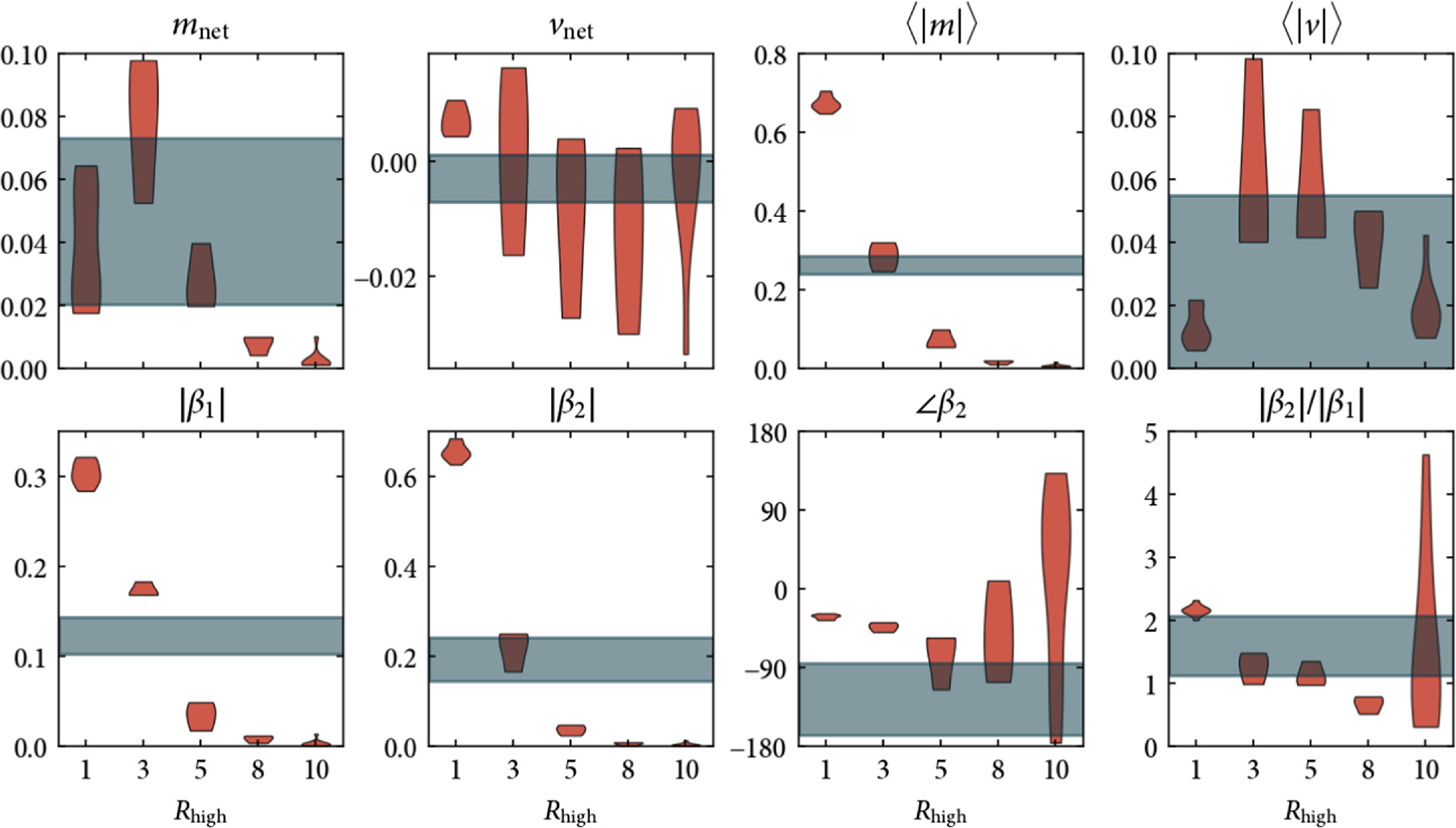
Figure 29. Distributions of observables for a selection of SANE models ray-traced with greater resolution in Rhigh between 1 and 10. These correspond to KHARMA SANE a* = − 0.5, i = 150° aligned models. We find rapid evolution in this part of parameter space.
Download figure:
Standard image High-resolution imageAppendix H: GRMHD Observable Distributions
To visualize trends of our eight observables in the five-dimensional parameter space that we explore, we provide "violin" plots of our observables from our models as a figure set, the complete version of which is available in the online journal. In each figure, we consider one observable and one magnetic field state (either MAD or SANE models). One figure, the distributions of mnet for MAD models, is shown in Figure 30. Different spins are shown in different columns, and different values of Rhigh are shown in different rows. Within each panel, we plot distributions as a function of inclination, where only five of the nine inclinations ray-traced in this work are included to improve readability. Aligned field models are shown on the left, and reversed field models are shown on the right. The distributions with opposite magnetic field polarity are usually very similar, with the notable exceptions of vnet and, more subtly, ∠β2. To display the relative agreement or disagreement between codes, we plot BHAC models in red and KHARMA models in blue. H-AMR models, which are ray-traced for a subset of models only for comparison here and not for scoring, are displayed as dashed distributions when available. Finally, the observational constraints are shown in gray, where, as usual, the allowed range for ∠β2 without RM derotation is shown as a hatched region.

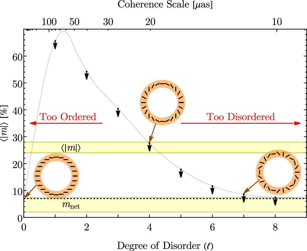
Figure 30.
Distributions of observables for either MAD or SANE models. BH spin a* varies in each column, and Rhigh varies in each row. Inclination varies along the x-axis. BHAC and KHARMA GRMHD simulations are shown in red and blue in each case, respectively, with H-AMR shown as a dashed curve. Distributions plotted on the left represent aligned magnetic fields, while those plotted on the right represent reversed magnetic fields. Our observational constraint is shown in gray. The complete figure set (18 images) is available in the online journal. (The complete figure set (18 images) is available.)
Download figure:
Standard image High-resolution imageOur last set of plots, distributions of the Faraday rotation depth  , are not directly observable but drive many of our physical trends, as well as differences between codes. For a detailed discussion of the physical trends present in these figures, we refer readers to Appendix A.
Differences between our KHARMA and BHAC models inflate our theoretical error bars in Section 5. We find that at least part of these differences arise from physical approximations regarding the assignment of electron temperature during the GRRT. One fluid with a single adiabatic index is evolved in our GRMHD codes, but it represents both relativistic electrons (with an adiabatic index of 4/3) and nonrelativistic ions (with an adiabatic index of 5/3). During the GRRT step of our calculations, only the electron temperature is relevant for the synchrotron emission that we observe. When assigning electron temperatures, RAPTOR adopts (see, e.g., Davelaar et al. 2018)

where Θe is the electron temperature, u is the internal energy, and R = Ti /Te given by Equation (8). Meanwhile, IPOLE accounts for the difference in adiabatic indices by adopting
where γe = 4/3 and γp = 5/3. Equation (H2) is physically justified, but it sacrifices internal consistency with the GRMHD simulations, where a single fluid with γ = 4/3 is evolved (Wong et al. 2022). When we set γe = γp = γ = 4/3 in Equation (H2), we recover Equation (H1) used by RAPTOR. Electron temperatures assigned by RAPTOR are systematically colder, 3/4 as hot as the ipole prescription at R = 1, and 1/2 as hot as R → ∞ . This explains the systematically larger Faraday depths in our BHAC models relative to both KHARMA and H-AMR, which are both ray-traced with ipole.
Larger differences are seen between SANE models than MADs. A unique SANE model is not believed to exist, and differences are known to occur at the GRMHD fluid level (Porth et al. 2019).
Footnotes
- 155
This toy model is equivalent to the "m-ring" model used in Paper VII, but we label with the index "ℓ" here to avoid ambiguities.
- 156
Rather than four-vector components, we average the Hodge dual of the Faraday tensor and then reconstruct the averaged magnetic field vector from the condition bμ uμ = 0.
- 157
The velocity is computed in the frame of the zero angular momentum observer in Boyer–Lindquist coordinates, while the magnetic field is computed in the fluid frame.
- 158
- 159
- 160
- 161
- 162
- 163
For ∠β2, to evade problems with phase wrapping, we translate angles into unit vectors in the complex plane centered at 0 before computing 90% quantiles and then translate back. If the magnitude of the mean of these unit vectors is less than 0.05, we set the lower and upper ranges of ∠β2 to −180° and 180°, respectively. This occurs predominantly when a model is so depolarized that its ∠β2 is approximately uniformly distributed.
- 164
Faraday rotation depth is obtained by integrating the radiative transfer coefficient of Faraday rotation, ρV , along each geodesic, and then performing an intensity-weighted average across the image (see, e.g., M87* Paper VIII).
- 165
For an aligned field model with i > 90°, the poloidal field is pointed away from us, leading to a systematic clockwise shift.