


Abstract
The Event Horizon Telescope observed the horizon-scale synchrotron emission region around the Galactic center supermassive black hole, Sagittarius A* (Sgr A*), in 2017. These observations revealed a bright, thick ring morphology with a diameter of 51.8 ± 2.3 μas and modest azimuthal brightness asymmetry, consistent with the expected appearance of a black hole with mass M ≈ 4 × 10⁶M⊙. From these observations, we present the first resolved linear and circular polarimetric images of Sgr A*. The linear polarization images demonstrate that the emission ring is highly polarized, exhibiting a prominent spiral electric vector polarization angle pattern with a peak fractional polarization of ∼40% in the western portion of the ring. The circular polarization images feature a modestly (∼5%–10%) polarized dipole structure along the emission ring, with negative circular polarization in the western region and positive circular polarization in the eastern region, although our methods exhibit stronger disagreement than for linear polarization. We analyze the data using multiple independent imaging and modeling methods, each of which is validated using a standardized suite of synthetic data sets. While the detailed spatial distribution of the linear polarization along the ring remains uncertain owing to the intrinsic variability of the source, the spiraling polarization structure is robust to methodological choices. The degree and orientation of the linear polarization provide stringent constraints for the black hole and its surrounding magnetic fields, which we discuss in an accompanying publication.
Export citation and abstract BibTeX RIS

Original content from this work may be used under the terms of the Creative Commons Attribution 4.0 licence. Any further distribution of this work must maintain attribution to the author(s) and the title of the work, journal citation and DOI.
1. Introduction
The Event Horizon Telescope (EHT) Collaboration, using the technique of very long baseline interferometry (VLBI) at 230 GHz, recently published the first resolved images of the supermassive black hole at the Galactic center, Sagittarius A* (Sgr A*). Analyses using a variety of imaging and geometrical modeling methods revealed a bright emission ring associated with the inner accretion flow together with a dark central brightness depression associated with gravitational lensing, redshift, and light capture by the black hole (Event Horizon Telescope Collaboration et al. 2022a, 2022b, 2022c, 2022d, 2022e, 2022f, hereafter Papers I–VI). Because Sgr A* is heavily scattered by the intervening ionized interstellar medium and exhibits rapid (intrahour) intrinsic variability, these analyses employed a series of novel approaches to address both effects on the emission morphology (see Papers II, III, and IV). These challenges, which were not relevant for EHT observations of Messier 87* (M87*; Event Horizon Telescope Collaboration et al. 2019a, 2019b, 2019c, 2019d, 2019e, 2019f, hereafter M87* Papers I–VI), led to substantial uncertainty in the resulting image, particularly in the azimuthal emission profile. Nevertheless, as discussed in Paper V, the diameter of the emission ring in Sgr A* is consistent with expectations for a black hole with a mass of M ≈ 4 × 10⁶ M⊙ located at a distance of D ≈ 8 kpc (e.g., Falcke et al. 2000; Broderick & Loeb 2005), as inferred by observations at infrared wavelengths of individual stellar orbits on scales of 103–105 Schwarzschild radii (Do et al. 2019; Gravity Collaboration et al. 2022).
The EHT images are broadly consistent with numerical simulations of a hot, radiatively inefficient, and highly sub-Eddington accretion flow (L/LEdd ∼ 10−9; Paper V). While initial evidence for a low accretion rate came from the radio and submillimeter spectrum of Sgr A* in total intensity (e.g., Falcke et al. 1993; Narayan et al. 1995; Yuan et al. 2003), the strongest evidence has come from polarimetric observations at radio and submillimeter wavelengths. The first polarized measurements of Sgr A* were made in circular polarization (Bower & Falcke 1999b).
155
Following these detections, initial measurements of linear polarization (Aitken et al. 2000; Bower et al. 2003) demonstrated that the accretion rate must be  yr−1 to avoid depolarization through Faraday rotation (e.g., Agol 2000; Quataert & Gruzinov 2000). Subsequent observations performed simultaneously at 227 and 343 GHz enabled measurements of the Faraday rotation measure (RM), RM ∼ − 5 × 10⁵ rad m−2 (Marrone et al. 2007), substantiating the low accretion rate and providing tighter constraints on models of the accretion flow. Studies of the polarimetric light curve of Sgr A* also revealed intrahour variability in the linear polarization (Marrone 2006; Marrone et al. 2008), circular polarization (Bower et al. 2002), and RM (Bower et al. 2018). The polarimetric variations occasionally show hints of loops in the Stokes
  -
- plane with a preference for clockwise motion, although counterclockwise motion is also regularly observed (Marrone et al. 2006b; Marrone 2006).
Unresolved polarimetric measurements of Sgr A* have also been made at near-infrared wavelengths, showing high fractional linear polarization with intrahour variability during flares (e.g., Genzel et al. 2003; Eckart et al. 2006; Trippe et al. 2007). Recently, the GRAVITY Collaboration produced polarimetric observations of the Galactic center in the near-infrared with the Very Large Telescope Interferometer (VLTI; Gravity Collaboration et al. 2017). These observations produced astrometric measurements suggestive of clockwise motion on the sky (Gravity Collaboration et al. 2018, 2023); the associated integrated polarization variability was consistent with models with a modestly inclined accretion flow and strong magnetic fields (Gravity Collaboration et al. 2020). The recent polarized light-curve studies by Wielgus et al. (2022b) at 230 GHz also support clockwise motion near the black hole, associated with an X-ray flare (Paper II; Wielgus et al. 2022a).
To date, the only spatially resolved polarimetric measurements of Sgr A* have come from precursor EHT observations at 230 GHz with a three-element array (Johnson et al. 2015). These observations found a sharp increase in the interferometric fractional polarization measured on long baselines, sometimes exceeding unity, indicative of synchrotron emission produced by partially ordered magnetic fields on scales of a few Schwarzschild radii (see also Gold et al. 2017). These observations also revealed intrahour variability in the interferometric fractional polarization on long baselines, indicating a compact and highly dynamic emission region. However, these observations did not have sufficient baseline coverage to produce images.
In this paper we present the first spatially resolved horizon-scale images of Sgr A* in linear and circular polarization, using EHT observations taken in 2017 April at a frequency of 230 GHz. In Section 2 we give an overview of the 2017 EHT observations and data processing. In Section 3 we discuss properties of the Sgr A* data set, and in Section 4 we discuss mitigation studies of three Sgr A*–specific challenges to the analysis. In Section 5 we give an overview of the analysis methods, and in Section 6 we present the linear and circular polarization images of Sgr A*. In Sections 7 and 8 we provide a discussion of the results and our main conclusions, respectively. Similar to the polarimetric analysis of M87* (Event Horizon Telescope Collaboration et al. 2021a, 2021b, 2023a, hereafter M87* Papers VII–IX), the polarized images of synchrotron emission from the immediate vicinity of the black hole event horizon provide a rich probe of the accretion physics and spacetime, which we discuss separately in an accompanying paper (Event Horizon Telescope Collaboration et al. 2024, hereafter Paper VIII).
2. Observations and Data Processing
The EHT observed Sgr A* on 2017 April 5, 6, 7, 10, and 11. The observatories participating in the 2017 campaign were the phased Atacama Large Millimeter/submillimeter Array (ALMA) and the Atacama Pathfinder Experiment (APEX) in the Atacama Desert in Chile, the James Clerk Maxwell Telescope (JCMT) and the phased Submillimeter Array (SMA) on Maunakea in Hawai'i, the Submillimeter Telescope (SMT) on Mt. Graham in Arizona, the IRAM 30 m (PV) telescope on Pico Veleta in Spain, the Large Millimeter Telescope Alfonso Serrano (LMT) on the Sierra Negra in Mexico, and the South Pole Telescope (SPT) in Antarctica (M87* Paper II). Sgr A* observations were interleaved with those of two calibrator sources, the quasars J1924−2914 and NRAO 530. Scientific analyses of EHT observations of these two calibrators are presented in Issaoun et al. (2022) and Jorstad et al. (2023), respectively. This letter focuses on Sgr A* observations on 2017 April 6 and 7, which have ALMA participation and low levels of variability in the source compared to the other observed days (Paper II).
The VLBI data were recorded in two polarizations and two frequency bands. All observatories recorded two 2 GHz-wide frequency bands centered at 227.1 and 229.1 GHz, to which we refer here as low and high band, respectively. A more detailed description of the EHT setup is presented in M87* Paper II. With the exception of ALMA and JCMT, all observatories recorded both right-circular polarization (RCP) and left-circular polarization (LCP). ALMA recorded dual linear polarization, which was later converted to circular polarization using the PolConvert software package (Martí-Vidal et al. 2016). JCMT recorded only RCP on April 5, 6, and 7 and LCP on April 10 and 11.
After correlating the recorded data from all telescopes, we corrected for instrumental bandpass effects and phase turbulence from Earth's atmosphere using established fringe-fitting algorithms (M87* Paper III). This calibration was carried out using two separate software pipelines: the CASA-based rPICARD (Janssen et al. 2019) and the HOPS-based EHT-HOPS (Blackburn et al. 2019). After the atmospheric phase variations are removed, the data can be coherently averaged in time to increase the signal-to-noise ratio (S/N). We also corrected for instrumental RCP and LCP phase and delay offsets by referencing the fringe solutions to phased ALMA (Martí-Vidal et al. 2016; Matthews et al. 2018; Goddi et al. 2019). The data were then amplitude-calibrated using station-specific measurements of the system equivalent flux density and time-averaged in 10 s segments (M87* Paper III; Paper II). Finally, stations with a colocated partner (i.e., ALMA, APEX, SMA, and JCMT) were "network-calibrated" to further improve the amplitude calibration accuracy (M87* Paper III; Blackburn et al. 2019). Calibrating Sgr A* presents unique challenges owing to its time-varying nature and extended emission on arcsecond scales, which can affect visibility amplitudes for baselines within local arrays like ALMA and SMA. Wielgus et al. (2022a) describe the techniques used to estimate the time-resolved flux density of Sgr A* to overcome these challenges during calibration. Gain amplitude corrections for the remaining stations were interpolated from solutions derived on the calibrator targets, J1924−2914 and NRAO 530 (Paper II).
The main goal of the subsequent polarimetric calibration is the correction of spurious polarimetric leakage. This step was not part of the initial total-intensity data analysis (Paper I), as the impact of leakage on the Stokes  component is negligible (Papers III and IV). Nonetheless, this effect is potentially significant for the analysis of linear and circular polarization. Hence, we employ the same calibration procedures used for M87* (M87* Paper VII) for the polarimetric analysis of the Sgr A* data. Since polarimetric leakage is an instrumental effect, the D-term coefficients, quantifying the impact of leakage on the data, are expected to be stable on timescales of the EHT observing campaign (∼1 week) and have the same values for all observed sources. ALMA is an exception because its polarimetric leakage is first corrected using multisource calibration as part of the PolConvert procedure, and the VLBI data are only impacted by residual leakage that can vary from day to day. Given these considerations, we apply precalculated D-terms to the Sgr A* data sets. For the stations with a colocated partner we use values derived through polsolve multisource fitting (Martí-Vidal et al. 2021) in Appendix D of M87* Paper VII, as shown in Tables 1 and 2. For all other stations except SPT, the adopted values shown in Table 3 are based on the M87* D-term ranges reported in Appendix E of M87* Paper VII as summarized in Issaoun et al. (2022). The SPT D-terms are assumed to be zero, consistent with the constraints from the analysis of the companion calibrators J1924−2914 and NRAO 530 (Issaoun et al. 2022; Jorstad et al. 2023), for which an identical set of D-terms was incorporated and verified through consistency tests.
Table 1. Daily Average D-terms for ALMA Derived Via the Multisource Intrasite Method
| Date | Band | DR (%) | DL (%) |
|---|---|---|---|
| Apr 5 | low | 0.30 − 2.80i (±0.70) | −1.42 − 3.74i (±0.70) |
| high | −0.17 − 4.10i (±0.60) | −1.09 − 4.02i (±0.60) | |
| Apr 6 | low | 0.60 − 5.45i (±0.40) | −0.53 − 6.08i (±0.40) |
| high | −0.09 − 1.52i (±0.30) | −0.75 − 1.66i (±0.30) | |
| Apr 7 | low | 1.12 − 7.10i (±0.70) | −0.46 − 5.77i (±0.70) |
| high | 1.25 − 4.93i (±0.70) | −0.37 − 4.00i (±0.70) | |
| Apr 10 | low | 0.78 − 2.61i (±0.30) | −0.40 − 2.82i (±0.30) |
| high | −0.02 − 3.04i (±0.30) | −0.56 − 3.92i (±0.30) | |
| Apr 11 | low | −0.15 − 6.33i (±0.50) | −0.80 − 6.09i (±0.50) |
| high | −0.29 − 5.19i (±0.40) | −0.76 − 5.07i (±0.40) |
Note. The D-term uncertainties are assumed to be distributed as circular Gaussians in the complex plane.
Download table as: ASCIITypeset image
Table 2. Campaign-average D-terms for APEX, JCMT, and SMA Derived via the Multisource Intrasite Method
| Station | DR (%) | DL (%) |
|---|---|---|
| APEX | −8.67 + 2.96i (±0.70) | 4.66 + 4.58i (±1.20) |
| JCMT | −0.09 − 2.29i (±1.80) | −0.46 + 3.34i (±0.60) |
| SMA | −1.73 + 4.81i (±1.00) | 2.79 + 4.00i (±2.20) |
Note. The D-term uncertainties are assumed to be distributed as circular Gaussians in the complex plane.
Download table as: ASCIITypeset image
Table 3. Leakage Calibration D-terms Assumed for Stations without a Colocated Site
| Station | DR (%) | DL (%) |
|---|---|---|
| LMT | 2.5 + 3.5i | −1.0 + 1.5i |
| SMT | 2.8 + 9.0i | −3.5 + 10.0i |
| PV | −13.0 + 3.5i | 15.0 + 0.0i |
Download table as: ASCIITypeset image
Finally, accurate calibration of complex R/L gain ratios is relevant particularly for circular polarization (Stokes  ) analysis. In this work we take a self-calibration approach that assumes
  . This method is more conservative regarding the potential detection of circular polarization than the primary approach discussed in Appendix A of M87* Paper IX. Nonetheless, this calibration allows for a full recovery of circular polarization morphology constrained by robust interferometric closure quantities; see also Roelofs et al. (2023).
3. Data Properties
In Figure 1, we show the (u, v) coverage and low-band interferometric polarization of the 2017 April 6 and 7 observations of Sgr A* as a function of (u, v) after D-term calibration. The colors encode the amplitude of the complex fractional polarization  in the visibility domain, coherently time-averaged in 120 s segments. Following Johnson et al. (2015), we define the visibility-domain fractional polarization as

where  ,
,  , and
, and  are the visibility-domain Stokes parameters sampled. Sgr A* is moderately polarized on most baselines,
  . Data points on the Chile–LMT and Chile–Hawai'i baselines for 2017 April 7 have very high fractional polarization,
  , that occurs at (u, v) spacings where the Stokes
  amplitudes approach a deep minimum. We also find that the polarization fractions on short (<3 Gλ) baselines are similar to those observed in 2013 by Johnson et al. (2015); see Figure 2.
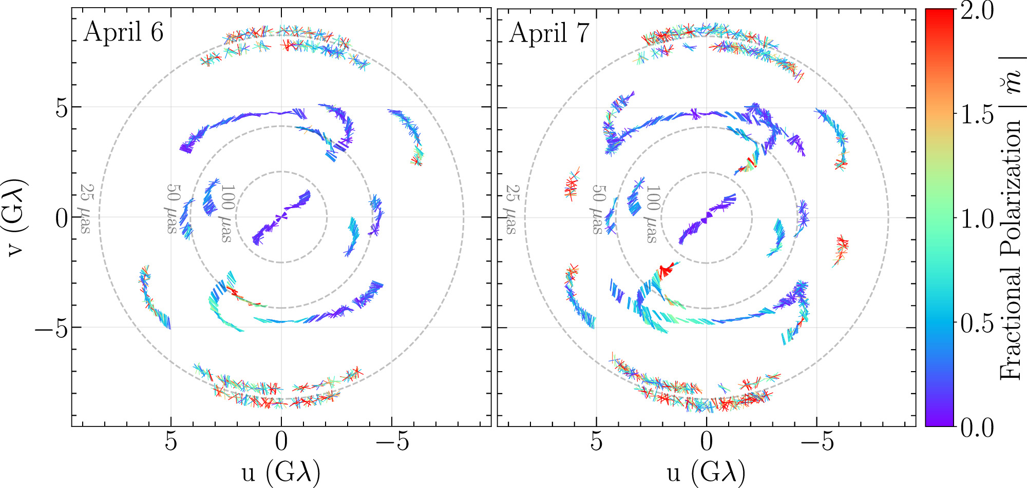
Figure 1. The (u, v) coverage for the April 6 (left) and April 7 (right) EHT observations of Sgr A* during the 2017 campaign. The color of the data points encodes the fractional polarization amplitude  in the range from 0 to 2, and the tick direction encodes the measured polarization direction
  . The data shown are derived from low-band visibilities after the data reduction and D-term calibration described in Section 2 have been applied. The data points are coherently averaged over 120 s. High polarization fractions at the tails of certain baseline tracks are due to low S/N, as they probe total-intensity minima.
Download figure:
Standard image High-resolution image
Figure 2. Comparison of the fractional linear polarization observed in precursor EHT observations on 2013 March 21 (left panel; Johnson et al. 2015) and similar spatial scales in our 2017 April 7 observations (right panel). The 2017 panel is a zoom-in of the right panel of Figure 1, with the color-bar amplitude range from Johnson et al. (2015).
Download figure:
Standard image High-resolution imageFigure 3 shows the phase of the conjugate closure trace products on two quadrangles (ALMA-APEX-LMT-SMT and ALMA-LMT-SMA-SMT, ordered as specified in Broderick & Pesce 2020) for the 2017 April 6 and 7 observations of Sgr A*. Closure traces are quantities immune to complex station gains and polarimetric leakages. Conjugate closure trace products deviate from unity (i.e., their phases deviate from zero) only in the presence of nonuniform polarization structures, and they are therefore clear indicators of source polarization (Broderick & Pesce 2020). We note significant deviations from zero in Figure 3, indicating that Sgr A* has spatially resolved, nonuniform polarization structure. Statistically different values of the conjugate closure trace products on the same quadrangles between 2017 April 6 and April 7 further indicate that the polarization structure in Sgr A* is time variable.
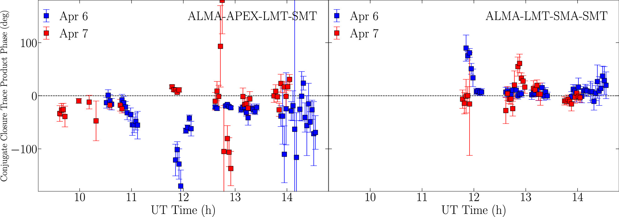
Figure 3. Conjugate closure trace product phases on two quadrangles for the April 6 and 7 observations of Sgr A*. The data points are coherently averaged across both frequency bands and in time over 120 s. Nonzero phases indicate that the source has spatially resolved and nonuniform polarized structure.
Download figure:
Standard image High-resolution imageIn Figure 4 (top panels), we show the RR* and LL* closure phases on two triangles with particularly high S/N. Significant deviations from zero are a consequence of resolved and asymmetric structure in RR* and LL*. The difference in closure phase between the two correlation products is shown in the bottom panels, with the average closure phase difference shown as a green band (1σ uncertainty in the estimate of the mean), which deviates from zero and thus indicates the presence of a circular polarization signal, as is the case for M87* (M87* Paper IX). Because the effects of residual uncorrected polarization leakage enter in at the ≲1% level for the parallel-hand correlation products, we expect the difference between RR* and LL* closure phases to be dominated by intrinsic Stokes  signal rather than by instrumental systematics. In fact, the study of systematics in the data in Paper II revealed an excess "noise" of RR* − LL* closure quantities in the Sgr A* data compared to other sources, likely due to the presence of intrinsic circular polarization in the source.

Figure 4. Closure phases observed on the ALMA-SMA-LMT (left) and ALMA-SMT-LMT (right) triangles during Sgr A* observations on April 6 (squares) and April 7 (circles). Open and filled markers denote low- and high-band data, respectively. Top: closure phases constructed from scan-averaged visibilities for both epochs, RR* in red, LL* in blue. Bottom: difference of closure phases between RR* and LL*. The zero level of the closure difference (i.e., no  detected) is marked with a black dashed line. The light-green band shows the average RR* − LL* difference.
Download figure:
Standard image High-resolution image4. Mitigation of Variability, Scattering, and Faraday Rotation in the Sgr A* Data
In comparison to the polarimetric analysis of M87* (M87* Paper VII), there are additional challenges in the Sgr A* data that increase the difficulty of reconstructing images. The effects of interstellar scattering along the line of sight to the Galactic center and the source's time variability on short (∼minutes) timescales have been studied and mitigated in the Stokes  analyses (Papers II, III, and IV). We discuss how the variability and scattering manifest in the polarimetric data in Sections 4.1 and 4.2, respectively. In Section 4.3, we discuss the additional effects of Faraday rotation on the results and how these inform theoretical interpretation.
4.1. Intrinsic Time Variability
4.1.1. Stokes  Variability

During the 2017 EHT observing campaign, Sgr A* exhibited Stokes  variability across a wide range of timescales. The compact source-integrated light curve during this period exhibits variability from minutes to the longest timescales probed (≳8 hr), with a "red" temporal power spectrum (i.e., larger variability on longer timescales; Wielgus et al. 2022a). Structural variability is also present on spatial scales comparable to that of the black hole shadow, appearing directly in visibility amplitudes and closure quantities (Papers II and IV).
The variability of Sgr A* was theoretically anticipated; the dynamical timescale near the event horizon of Sgr A* is ∼GM/c3 ≈ 20 s, and the observed brightness fluctuations are natural consequences of the turbulent structures predicted by numerical general relativistic magnetohydrodynamic (GRMHD) simulations (Paper V). A survey of the EHT simulation library confirms that the spatiotemporal power spectrum of the variability (i.e., fluctuations about the mean image) in the GRMHD simulations is universally well approximated by a cylindrically symmetric, broken power law in both the spatial and temporal dimensions (Georgiev et al. 2022). These power laws are dominated by the largest spatial and longest temporal scales, i.e., they exhibit a "red"-"red" power spectral density. As a consequence, in the GRMHD simulations, the bulk of the variability can be eliminated by normalizing the total intensity of individual image frames (Wielgus et al. 2022a). After light-curve normalization, the intranight power spectrum peaks at a baseline length of ≲2 Gλ (≳100 μas).
Tools for measuring and mitigating the Stokes  variability in Sgr A* have been developed based on the universality observed in GRMHD simulations (Broderick et al. 2022). The spatial power spectra have been estimated by computing means and variances of visibility amplitudes across frequency bands and days in patches of the (u,v) plane after light-curve normalization and performing linear debiasing (see Section 4 of Broderick et al. 2022). This procedure leverages the compact nature of Sgr A*, makes use of the approximate spatial isotropy anticipated from the GRMHD simulations (Georgiev et al. 2022), and incorporates estimates of the uncertainty that include contributions from the statistical error (i.e., thermal noise), gain amplitudes, and leakage terms (D-terms). Because the number of data points in any range of baseline lengths can be small, this estimator can suffer from known biases that may be corrected via calibration with appropriate mock data sets (Paper IV). Upon doing so, the resulting empirical estimates of the structural variability power spectrum match those from GRMHD simulations in amplitude and shape (Paper V).
156
variability in Sgr A* have been developed based on the universality observed in GRMHD simulations (Broderick et al. 2022). The spatial power spectra have been estimated by computing means and variances of visibility amplitudes across frequency bands and days in patches of the (u,v) plane after light-curve normalization and performing linear debiasing (see Section 4 of Broderick et al. 2022). This procedure leverages the compact nature of Sgr A*, makes use of the approximate spatial isotropy anticipated from the GRMHD simulations (Georgiev et al. 2022), and incorporates estimates of the uncertainty that include contributions from the statistical error (i.e., thermal noise), gain amplitudes, and leakage terms (D-terms). Because the number of data points in any range of baseline lengths can be small, this estimator can suffer from known biases that may be corrected via calibration with appropriate mock data sets (Paper IV). Upon doing so, the resulting empirical estimates of the structural variability power spectrum match those from GRMHD simulations in amplitude and shape (Paper V).
156
The intrahour structural variability of Sgr A* was mitigated in Paper III in three stages. First, the complex visibilities were light-curve normalized (Wielgus et al. 2022a), eliminating the largest component of the variability and suppressing all correlated components. Second, the additional variability power, inferred from the empirical variability estimate, was introduced as an additional statistical error about a mean image structure. Where the magnitude of this additional component was uncertain, the level of excess "noise" was surveyed as part of the imaging and modeling exploration. Third, the additional uncertainty necessary was estimated via "noise-modeling," the direct fitting of a simultaneous model for the mean image and a parameterized, broken power-law model for the statistical properties of the otherwise unmodeled variability (Broderick et al. 2022; Paper IV).
4.1.2. Polarimetric Variability
Consistent with historical expectations (e.g., Bower et al. 2002; Marrone et al. 2006a), during the 2017 EHT campaign Sgr A* exhibited significant polarimetric variability. This variability is strongly implied by the rapid fluctuations
157
in the measured polarization direction in Figure 1. Variability is also shown explicitly in Figure 5 for the crossing and following tracks identified in Paper IV—segments of baseline tracks that substantially overlap at different observing times throughout the night—for which large polarization direction swings are present on timescales ≳3 hr, including large differences between 2017 April 6 and 7. Polarimetric variability is similarly implied by the rapid variations in the conjugate closure trace products shown in Figure 3, and it is shown explicitly by the comparison between observation days. For both of the quadrangles shown in Figure 3, the phase of the conjugate closure trace products varies by ∼90° on timescales of tens of minutes, on similar timescales to the variability observed in Stokes  but lower in magnitude.
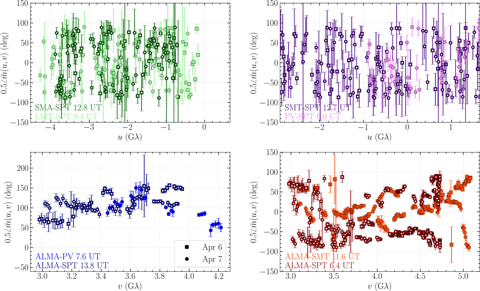
Figure 5. Phase of  on the crossing and following tracks identified in Paper IV, during which the same (u,v) positions are sampled at different times by different baselines on 2017 April 6 (squares) and 7 (circles). The central time stamps for each track are labeled in the corresponding colors (see Figure 2 of Paper IV for exact track locations in the (u,v) plane). All data have been coherently averaged on 120 s timescales to illustrate short-timescale variability. No additional systematic uncertainty has been added.
Download figure:
Standard image High-resolution imageTo quantitatively assess the degree of polarimetric variability, we extend the empirical estimate used for Stokes  from Broderick et al. (2022) to the independent parallel-hand and cross-hand correlation products. Following the application of calibrator-determined leakage terms, the procedure is similar to that in Paper IV: visibilities are scan-averaged and light-curve normalized, the mean and variance within patches are computed after linear detrending and azimuthally averaged, and uncertainties are estimated via Monte Carlo sampling of the statistical uncertainties, complex gains, and leakages. Estimates of the azimuthally averaged power spectra are independently generated for RR*, LL*, RL*, and LR*. The results after combining the 2017 April 6 and April 7 data are shown in Figure 6 for each hand independently.
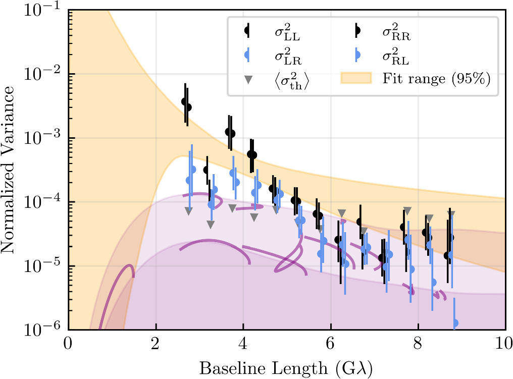
Figure 6. Model-agnostic estimates of the azimuthally averaged excess variance of the parallel-hand and cross-hand visibility amplitudes, after removing that from the reported statistical errors, as a function of baseline length. Nonparametric estimates are obtained across April 6 and 7, using both high- and low-band data. Uncertainties associated with the thermal errors, uncertain station gains, and polarization leakage are indicated by the error bars. Azimuthally averaged thermal errors are shown by the gray triangles and provide an approximate lower limit on the range of accurate variance estimates. For comparison, the magnitudes of the variance induced by refractive scattering are shown in purple along the minor (top) and major (bottom) axes of the diffractive scattering kernel (see Section 4 of Paper III); the variance along individual tracks on April 7 is shown by the solid purple lines. The orange band indicates the 95th percentile range of broken power-law fits to the Stokes  excess variances from Paper IV.
Download figure:
Standard image High-resolution imageThe empirically estimated parallel-hand power spectra (RR* and LL*) are statistically indistinguishable from each other and from those associated with their Stokes  counterpart. This similarity implies that the absolute variability in Stokes
  on ≲50 μas is small in comparison to the variability in Stokes
  . Practically, it implies that variability in the parallel hands may be mitigated effectively using the model in Papers III and IV for RR* and LL* individually.
The cross-hand power spectra (RL* and LR*) are statistically indistinguishable from each other. In the absence of uncorrected leakage, this is expected by construction and thus provides additional confidence in the calibrator-implied D-terms. More importantly, the cross-hand power spectra share the shape of those associated with the parallel hands, though rescaled to approximately 50% of the parallel-hand amplitude.
As in Papers III and IV, we employ multiple variability mitigation schemes when modeling or imaging the Sgr A* data. These may be segregated into two general categories:
- Post-marginalization: Multiple images are reconstructed on subsets of the data that span sufficiently short periods of time that variability may be ignored, and they are subsequently combined to yield a single "average" image.
- Pre-marginalization: A single image is fit to the entire data set, with additional noise added to account for the deviations in the visibilities due to the structural variability in addition to the statistical and systematic components.
For the pre-marginalization methods, we make use of the empirical polarimetric variability power spectra in a way similar to Paper III, modified for polarimetric reconstructions. As with Stokes  , we normalize all correlation products by the Stokes
  light curve to reduce the impact of large-scale correlated variability. Additional statistical error following the broken power-law model is then added in quadrature to each correlation product, with the parallel hands receiving the same additional noise as applied to Stokes
  and cross-hands receiving an amount that is reduced by a fixed fraction.
For Sgr A* the parallel-hand/cross-hand variance ratio is 50%, i.e., half as much noise is added in an absolute sense to the cross-hands as that added to the parallel hands. 158 Depending on the polarimetric image reconstruction method, parameters of the additional noise model are surveyed or directly reconstructed (see Appendix A). Moreover, the value of this variance ratio depends on the source properties and can be both much smaller and larger for other data sets (e.g., the synthetic data sets discussed in Appendix B) than found for Sgr A*, depending on both the polarization fraction and degree of variability.
4.2. Interstellar Scattering
At radio wavelengths, the image of Sgr A* is heavily scattered by ionized interstellar plasma along the line of sight. In particular, density inhomogeneities result in a variable index of refraction, with corresponding phase fluctuations across an image that vary with time and observing wavelength (δ ϕ ∝ λ). For detailed discussion and a historical summary of the scattering of Sgr A*, see Psaltis et al. (2018) and Johnson et al. (2018).
The effects of scattering are predominantly caused by inhomogeneities on two widely separated spatial scales. "Diffractive" scattering arises from fluctuations on spatial scales of ≲ 103 km and results in blurring of the image with an approximately Gaussian kernel. "Refractive" scattering arises from fluctuations on spatial scales of ≳ 107 km and results in irregular distortion of the image that does not correspond to a convolution. In terms of interferometric visibilities, the signal on long baselines is exponentially suppressed by diffractive blurring but retains an additive contribution from refractive "noise" (Goodman & Narayan 1989; Narayan & Goodman 1989; Johnson et al. 2015; Johnson & Narayan 2016). In this paper, we follow the approach used in previous papers in this series and "deblur" our data before imaging (see, e.g., Fish et al. 2014), dividing each measurement by the Fourier-conjugate scattering kernel on its baseline; we use the scattering kernel parameters from Johnson et al. (2018), which have been estimated using historical measurements of Sgr A* and validated by subsequent measurements (Issaoun et al. 2019, 2021; Cho et al. 2022). See Paper II for more details on the effects of interstellar scattering for EHT Sgr A* data.
Because the ionized interstellar medium is not significantly birefringent (e.g., Thompson et al. 2017; Ni et al. 2022), the effects of scattering on polarimetric observables can be mild. For example, interferometric fractional polarization is invariant to diffractive blurring; other image-integrated properties, such as the rotationally symmetric mode (β2) that we analyze extensively in Paper VIII, are only mildly affected by blurring (Palumbo et al. 2020). In general, the interferometric fractional polarization is only weakly affected for any baseline on which refractive noise is small compared to the signal amplitude (see, e.g., Ricarte et al. 2023). Moreover, because the beam of the EHT is comparable to the size of the diffractive blurring kernel, the effects of scattering on the polarized image of Sgr A* are expected to be mild when viewed at the resolution of the EHT. Figure 7 shows example scattered images of GRMHD simulations in linear and circular polarization.
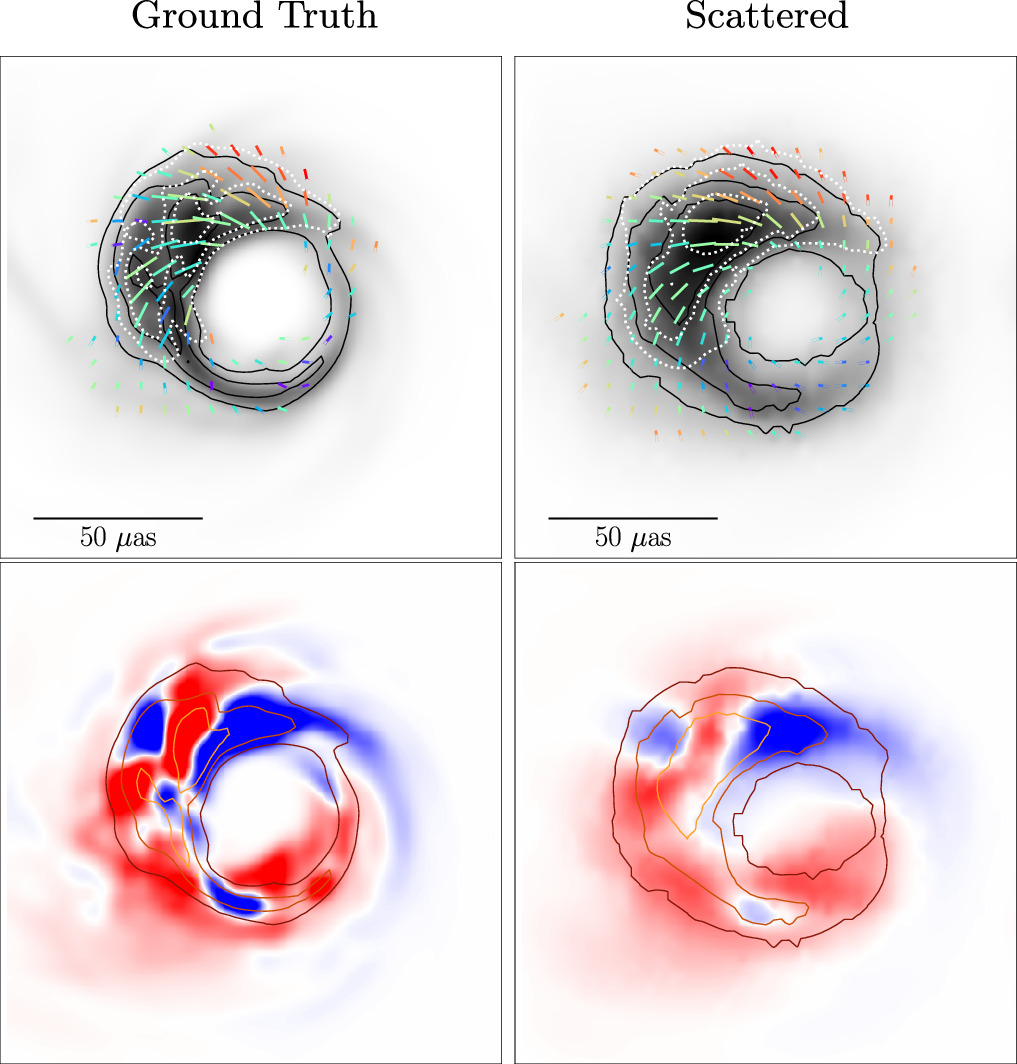
Figure 7. A comparison of GRMHD simulation snapshots in linear (top) and circular (bottom) polarization with and without the effects of interstellar scattering. Associated measurable quantities are given in Table 4. For display purposes the unscattered snapshots are blurred with a small 5 μas circular Gaussian beam, much smaller than the EHT instrument resolution. Top: total intensity is shown in gray scale, polarization ticks indicate the EVPA, the tick length is proportional to the linear polarization intensity magnitude, and color indicates fractional linear polarization. The dotted contour levels correspond to linearly polarized intensities of 25%, 50%, and 75% of the polarization peak. Cuts are made to omit all regions in the images where Stokes  % of the peak brightness and
  10% of the peak polarized brightness. Bottom: total intensity is indicated in colored linear-scale contours, and the Stokes
  brightness is indicated in the diverging color map, with red/blue indicating a positive/negative sign.
Download figure:
Standard image High-resolution imageTable 4 shows the values of the image quantities useful in polarimetric model discrimination in unscattered, scattered, and blurred images of a GRMHD simulation viewed at 230 GHz. We define the image-integrated net linear and circular polarization fractions as


where the sum is over the pixels indexed by i. We also measure the image-averaged linear and circular polarization fractions 〈∣m∣〉 and 〈∣v∣〉 across the images:


Note that these quantities depend on the resolution of the image; high-resolution GRMHD images will have systematically larger polarization fractions than their counterpart image reconstructions. All images used for analyses in this paper and the companion Paper VIII have been blurred to an effective resolution of 20 μas. Following Palumbo et al. (2020), we also compute complex βm modes, which are Fourier decompositions of the linear polarization structure:

where (ρ, φ) are polar coordinates in the image plane and  is the total flux density in the image. The β1 mode is the simplest asymmetric mode, while β2 is the simplest rotationally symmetric mode. In particular, ∠β2 is a probe of the handedness and pitch angle of the overall twist of the electric vector polarization angle (EVPA) pattern, where ∠β2 = 0° indicates a radial EVPA pattern and ∠β2 = 180° indicates a toroidal EVPA pattern on the image.
Table 4. Image Quantities of Interest Computed on a Snapshot of a GRMHD Simulation with and without Interstellar Scattering Effects
| Param. | Intrinsic | Blurred | Scattered and Blurred |
|---|---|---|---|
| ∣mnet∣(%) | 4.72 | 4.72 | 4.62 |
| vnet(%) | 0.33 | 0.33 | 0.35 |
| 〈∣m∣〉(%) | 49.66 | 31.97 | 31.82 |
| 〈∣v∣〉(%) | 2.26 | 0.91 | 0.93 |
| ∣β1∣ | 0.14 | 0.14 | 0.14 |
| ∣β2∣ | 0.34 | 0.30 | 0.29 |
| ∠β2 (deg) | 93.8 | 92.5 | 92.4 |
| ∣β2∣/∣β1∣ | 2.43 | 2.15 | 2.14 |
Note. The GRMHD simulation is a magnetically arrested disk model with a* = 0.5, Rlow = 1, and Rhigh = 80 viewed at 30° inclination before and after interstellar scattering (Event Horizon Telescope Collaboration et al. 2022e). In the middle column, the image is blurred by a 20 μas circular Gaussian beam. In the right column, the simulated effects of scattering are applied, which produces diffractive blurring at sub-beam scales. Additional circular Gaussian blurring is performed to reach the 20 μas imaging resolution. The field of view and pixel size are the same in each case.
Download table as: ASCIITypeset image
Image-integrated quantities such as ∣mnet∣ change very little, while resolved quantities such as 〈∣m∣〉 are significantly diminished by the diffractive blurring depolarization caused by scattering. Notably, low-resolution morphological quantities like β1 and β2 are almost completely unaffected, particularly in phase, though higher-order modes would be more disrupted. However, the effective size of the scattering kernel, ∼16 μas, is below the effective instrument resolution of ∼20 μas, and so the presence of scattering is not a large contaminant of the image quantities of interest.
4.3. Faraday Rotation
As radiation propagates through a magnetized medium, the polarization state is affected by Faraday effects. Most notably, the EVPA changes because of Faraday rotation, quantifiable with an RM. The RM can be characterized as

a difference in measured EVPAs χ1,2 between the frequency bands corresponding to wavelengths λ1,2 (e.g., Brentjens & de Bruyn 2005). A large RM of ∼ − 4 × 10⁵ rad m−2 has been measured in Sgr A* at 230 GHz. While the measured value of RM fluctuates significantly, the observed negative sign has remained consistent for decades (e.g., Bower et al. 2018; Wielgus et al. 2024). Detailed RM measurements from ALMA as a connected-element interferometric array are available for the exact EHT observing epochs, which indicate values consistent with historical data (Goddi et al. 2021; Wielgus et al. 2022b, 2024); see Table 5.
Table 5. Median Rotation Measure of Sgr A* Obtained from the ALMA Interferometric Light Curves (Wielgus et al. 2022b)
| Observations | RM (105rad m−2) | ΔEVPA (deg) |
|---|---|---|
| April 6 | −4.87
| −48.2
|
| April 7 | −4.56
| −45.1
|
| April 11 | −3.15
| −31.2
|
| April 6, 7 | −4.65
| −46.0
|
| All Days | −4.23
| −41.9
|
Note. The error estimates correspond to 68% of the distribution. The change in EVPA is evaluated at 228.1 GHz.
Download table as: ASCIITypeset image
If the entire RM can be confidently attributed to an external Faraday screen located between the emitting compact source and Earth, then the intrinsic EVPA pattern can be recovered by simply "derotating" EVPA ticks by an amount −RMλ2. For these observations, the measured RM assuming an entirely external screen leads to rotating the observed EVPAs by approximately 50° (Table 5) clockwise before comparing them to theoretical models of the accretion flow near the black hole event horizon. The external character of the Faraday screen is supported by the persistence of the RM sign over long timescales, since we would expect frequent sign reversals in the turbulent accretion flow near the event horizon (Ricarte et al. 2020; Ressler et al. 2023). On the other hand, Wielgus et al. (2022b) reported time-resolved Faraday rotation, with the inferred RM fluctuating by up to 50% on subhour timescales. These results point toward at least some of the Faraday rotation being due to an internal Faraday screen cospatial with the observed compact emitting region (Wielgus et al. 2024). In this limit, no EVPA derotation is required before comparing models to observations, as the theoretical models of the compact emission zone should fully account for the observed Faraday rotation.
A concordance picture could involve a slowly varying external Faraday screen to maintain a constant sign on relevant timescales in addition to an internal Faraday screen of a similar magnitude to explain the rapid time variability (Ressler et al. 2023). In this picture, it is justified to derotate the EVPA ticks by the median RM measured for a given observation, as the duration of the observing night is much longer than the dynamical timescale near the event horizon of Sgr A*. Furthermore, because of the rapid variability of the RM measured by ALMA (Wielgus et al. 2022b), the amount of EVPA corruption changes in time by about ±15° (Table 5). This further inflates uncertainties of the inferred EVPA structure in the reconstructed images and can be captured in data-driven estimates of polarimetric variability discussed in Section 4.1.2. These considerations are crucial for theoretical interpretation of the EHT results, and we investigate the impact of Faraday rotation in more detail using simulations in Paper VIII.
5. Methods
In this section, we present a summary of the methods used for the Sgr A* polarimetry results. We carry out geometric modeling of the source with a snapshot m-ring model fitting method (Paper IV; Roelofs et al. 2023). We additionally use three imaging methods: the Bayesian imaging framework Themis (Broderick et al. 2020, 2020c) and the regularized maximum likelihood (RML) methods eht-imaging (Chael et al. 2016, 2018) and DoG-HiT (Müller & Lobanov 2022). These methods are inherently different from one another in how they handle the intrinsic variability of the source. We summarize here the main method characteristics; more detailed descriptions can be found in Appendix A.
As a continuation of the analysis performed in the total-intensity companion papers (Papers III and IV), we model the polarization structure on top of a ring morphology, inferred through the analysis of the total-intensity observations. To aid in the total-intensity reconstruction step, the RML imaging methods use Sgr A* data sets that have been self-calibrated to the fiducial average deblurred total-intensity image produced with the image clustering procedure in Section 7.2 of Paper III. Tests of the effect of the various ring cluster modes on the polarimetric structure reconstructions, which is minimal, are shown in Appendix C. The Themis and snapshot m-ring methods do not use the self-calibrated data and do their own self-calibration simultaneously with the data fitting. All methods make use of data that have been D-term calibrated, light-curve normalized, and deblurred to counter the effects of diffractive scattering and prescribe an appropriate total-intensity and polarization noise budget following the variability studies described in Section 4.1.
5.1. Snapshot m-ring Modeling
With the snapshot m-ring modeling method, we fit a polarimetric geometric model ("m-ring"; see Appendix A for details) to 2-minute snapshots from our data sets (Paper IV; Roelofs et al. 2023). We only use snapshots with at least 10 visibilities and 60 s of coherent integration time. After time-averaging the snapshots to 120 s, 2% of the visibility amplitudes are added to the thermal noise budget in order to represent systematic uncertainties. We fix the leakage parameters to the predetermined solutions from the EHT polarimetric M87* analysis; see Section 2. For our linear polarization fits, we fit our m-ring model to closure phases, closure amplitudes, and the visibility-domain fractional linear polarization  for each snapshot independently (i.e., no temporal correlations are assumed). For our circular polarization fits, we fix the linear polarization parameters to the maximum a posteriori (MAP) estimates and fit to the parallel-hand closure phases and closure amplitudes (i.e., we fit to the separate RR* and LL* closure products). We also explore fits to RR*/LL* visibility ratios. All these data products are robust to multiplicative station gains, except the RR*/LL* visibility ratios, which may be affected by residual R/L gain ratios (see also tests carried out in Roelofs et al. 2023). After fitting each snapshot from each day and frequency band, we combine all posteriors to a single posterior using a Bayesian averaging scheme (Paper IV).
5.2. THEMIS
As described in Broderick et al. (2020) and M87* Paper VII, the Themis image model consists of a rectilinear set of control points, spanned via a bicubic spline. Raster orientation and field of view are free parameters and dynamically adjust during image reconstruction to choose an effective resolution. Raster resolution is determined by maximizing the Bayesian evidence over the raster dimension; typically, this is small owing to the limited number of EHT resolution elements across Sgr A*, and we make use of a 7 × 7 raster based on the Stokes  study in Paper III. The full polarimetric image model consists of four identically sized and oriented rasters that specify the total intensity, polarization fraction, EVPA, and Stokes
  . As described in Broderick et al. (2022) and Section 4.1.2, intrinsic source variability is mitigated via the modeling of a parameterized additional baseline-dependent contribution to the data uncertainties. The uncertainty model is composed of components that correspond to the variability noise, the refractive scattering noise, and the systematic error budget (see, e.g., Paper IV).
Themis reconstructions are fit directly to the scan-averaged complex visibilities (RR*, LL*, RL*, LR*), after light-curve normalization as described in Section 4.1.2, combined across bands and 2017 April 6 and 7. Simultaneous with image generation, leakage terms and complex gains are recovered. To avoid complications from potential night-to-night variations in the D-terms at ALMA and SMA, we fit data that are precorrected using the M87* Paper VII leakages. However, during fitting, D-terms that are constant across both observation days and high and low bands are obtained from Sgr A* alone and do not further incorporate prior leakage estimates from other source reconstructions. Complex station gains are reconstructed independently on scans and across bands but are restricted to have unit R/L gain ratios. Synthetic data tests reported in M87* Paper IX on Stokes  in M87* showed that R/L gain discrepancies of more than a few percent produced fits noticeably worse than those with smaller discrepancies. Themis images produced good-quality fits to EHT data; thus, R/L gain offsets are expected to be very small.
The result of Themis fits is an approximate posterior composed of a set of images that may be used for Bayesian interpretation. For more details on likelihood construction, sampling, and chain convergence criteria see Appendix A and references therein.
5.3. Eht-imaging
The eht-imaging (Chael et al. 2016, 2018) package is a pixel-based RML imaging algorithm. Reconstructions are done via minimization of an objective function through gradient descent. This objective function is constructed with χ2 goodness-of-fit terms and regularizer terms that favor or penalize specific image properties. For polarized image reconstructions, we adopt a very similar methodology to the polarimetric imaging of M87*, described in Appendix C of M87* Paper VII. Since leakage is already corrected in the Sgr A* data from the M87* analysis, this step is omitted. We use the data self-calibrated to the fiducial total-intensity image as our starting data sets. These data are self-calibrated to a deblurred image, so no scattering mitigation is done as part of our procedure. We coherently average the data for 120 s, combine high and low bands into a single data set, and reconstruct one image per observing day for April 6 and 7. We add a fractional systematic noise budget of 5% based on the total-intensity parameter exploration (see Table 4 of Paper III). We also add the variability noise budget determined in the total-intensity efforts in quadrature to the uncertainty of each visibility point (see Section 3.2.2 of Paper III), halving the budget applied to cross-hand visibilities based on the polarimetric variability assessment in Section 4.1.2.
As a first step, we reconstruct a starting total-intensity image by fitting to parallel-hand closure phases, closure amplitudes, and visibility amplitudes. This total-intensity image is then kept fixed during the polarimetric imaging, defining the regions where polarimetric intensity is allowed. The imaging is done via iterative rounds of gradient descent. At each iteration, the output image is blurred with a 20 μas Gaussian beam and used as the initial image for the next round, and the weights on the data terms are increased. Linear polarimetric imaging and circular polarimetric imaging are done separately. For linear polarization, we fit the RL* polarimetric visibility  and the visibility-domain polarimetric ratio
  . For circular polarization, we fit the self-calibrated
  visibilities and the parallel-hand closure phases and closure amplitudes, and we solve for right and left complex gains independently.
5.4. DoG-HiT
The DoG-HiT package (Müller & Lobanov 2022, 2023a, 2023b) is a wavelet-based imaging algorithm that uses compressive sensing. DoG-HiT fits the χ2 data terms while assuming that the image structure is sparsely represented by a small number of wavelets. For the polarimetric and dynamic analysis we follow the description presented in Müller & Lobanov (2023b). Similar to the procedure for eht-imaging outlined in Section 5.3, we use the band-averaged, self-calibrated, and leakage-corrected data set as a starting point. No scattering mitigation was applied as part of the procedure. We add a fractional systematic noise budget of 2% to the 120 s averaged visibilities.
First, we recover a mean Stokes  image with DoG-HiT, only fitting to the closure phases and closure amplitudes computed from the Stokes I visibilities. We self-calibrate residual gains to this image on 10-minute intervals, and we derive the multiresolution support, i.e., the set of significant wavelet coefficients, from the mean image. The multiresolution support fixes the spatial scales and positions for the dynamic and polarimetric imaging where emission is allowed. Next, we construct a mean polarimetric image by fitting the polarimetric visibilities
  and
and  , but we only allow wavelet coefficients in the multiresolution support to vary. In an iterative procedure, we solve for residual D-terms. Finally, we cut the observation into frames of 30 minutes and fit the total-intensity and polarimetric visibilities in each frame independently starting from the mean images, but we only vary wavelet coefficients in the multiresolution support. We average the recovered frames uniformly to achieve a final static image. The whole procedure is carried out for both days of observations independently and finally averaged.
5.5. Synthetic Data Tests
All methods are validated against synthetic data sets that mimic properties of Sgr A*, the results of which are presented in detail in Appendix B. Two GRMHD models are chosen from the passing set of Sgr A* theoretical models that mimic both total-intensity and polarization properties of the source. One model has lower total linear polarization than Sgr A* but has a similar variability ratio of the cross-hand compared to the parallel-hand visibilities, while the other model has a total linear polarization fraction similar to that of Sgr A* but has a higher variability ratio of the cross-hands compared to the parallel hands. As discussed in Paper V, the variability in the GRMHD simulations is generally higher than for Sgr A*, making synthetic data more challenging to reconstruct than the real data. All methods are able to reconstruct the linear polarization structure of the two models, while Themis and the snapshot m-ring modeling methods fare better in reconstructing the circular polarization structure. Since Themis and m-ring modeling both carry out posterior exploration as part of their methodologies, they provide tight posterior distributions and measured uncertainties on individual linear and circular polarization quantities. These two methods are thus selected as the primary methods for analysis and theoretical interpretation, while the two RML methods are presented as additional validation methods.
6. Results
6.1. Linear Polarization
In Figure 8, we present the Sgr A* linear polarimetric images produced by each method, combining bands and observing days. The main results are produced using data processed through the EHT-HOPS pipeline, and consistency tests with the CASA rPICARD pipeline are presented in Appendix D. The Bayesian imaging method Themis produces an average image from many individual posterior draws with both days and bands combined into one data set. The snapshot modeling method produces an average image by combining individual band-combined snapshots across both days using Bayesian posterior averaging. Because the m-ring is a simple geometric model, the structure appears less noisy than the other methods. The RML imaging methods eht-imaging and DoG-HiT produce band-combined images per day; we display here the average image over 2 days (i.e., the April 6 and 7 images averaged together after imaging). In Figure 9, we present the same images but with EVPAs rotated by a constant angle to account for the median Faraday rotation in the combined April 6 and 7 data set, corresponding to a clockwise rotation of the EVPA by 46.0 deg, as discussed in Section 4.3.
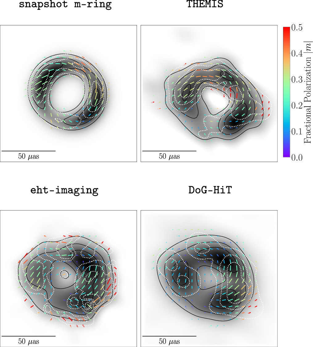
Figure 8. Linear polarimetric images of Sgr A* from the combined 2017 April 6 and 7 observations with the primary methods snapshot m-ring modeling and Themis and the validation methods eht-imaging and DoG-HiT. The posterior-average image is shown for the posterior exploration methods. Total intensity is shown in gray scale, polarization ticks indicate the EVPA, the tick length is proportional to the linear polarization intensity magnitude, and color indicates fractional linear polarization. The white dotted contours mark the linear polarized intensity, corresponding to 25%, 50%, and 75% of the polarization peak. We have masked out all regions in which Stokes  % of the peak brightness, and we have similarly masked out all regions in which
  10% of the peak polarized brightness, where
  . The color-bar range is fixed for all panels.
Download figure:
Standard image High-resolution image
Figure 9. Polarimetric images of Sgr A* from Figure 8, but with EVPAs rotated by 46.0 deg to account for the median Faraday rotation in the combined April 6 and 7 data set (Table 5). The color-bar range is fixed for all panels.
Download figure:
Standard image High-resolution imageThe Sgr A* emission ring is almost entirely polarized, with a peak fractional polarization of ∼40% at ∼20 μas resolution in the western region of the ring. The m-ring model shows a more prominent northwest peak due to the symmetry of the model m-mode; see Appendix A. The polarized emission EVPA pattern along the ring is nearly azimuthal with a counterclockwise handedness that is robust across time, frequency, and analysis method.
In Figure 10, we show the average of the four method images combining bands and days shown in Figure 8. The averaging is done independently for each Stokes intensity distribution. Due to the m-ring image having lower net polarization fraction (an effect of the variability of the EVPAs in snapshot averaging), the peak polarization fraction in the average image is lower than those of individual methods. This image is adopted as the conservative representation of the overall Sgr A* linear polarization structure, while individual method images are used for quantitative comparisons and theoretical interpretation; see Section 7 and Paper VIII.
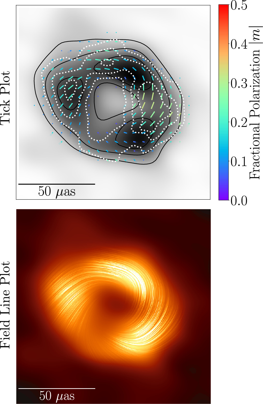
Figure 10. Top: linear polarization image of Sagittarius A*. This image is the band, day, and method average of the linear polarization structure reconstructed from 2017 April 6 and 7 EHT observations. The display choices are analogous to Figure 8. Bottom: polarization "field lines" plotted atop an underlying total-intensity image. Treating the linear polarization as a vector field, the sweeping lines in the images represent streamlines of this field and thus trace the EVPA patterns in the image. To emphasize the regions with stronger polarization detections, we have scaled the length and opacity of these streamlines as the square of the polarized intensity. This visualization is inspired in part by line integral convolution (Cabral & Leedom 1993) representations of vector fields. The average linear polarization structure is overlaid on the fiducial average total-intensity image from Paper I.
Download figure:
Standard image High-resolution image6.2. Circular Polarization
In Figure 11, we present the circular polarization images produced by each method, combining bands and observing days. In the chosen color map, red and blue correspond to positive and negative circular-polarized flux density, respectively, with contours indicating the Stokes  brightness. As in the synthetic data tests shown in Appendix B, the circular polarization structure is consistent for the snapshot m-ring and Themis posterior exploration methods, while the RML imaging methods show some differences. All methods see prominent negative circular polarization in the western portion of the ring, while only the snapshot m-ring and Themis methods recover positive circular polarization in the northeast region of the ring. The m-ring and Themis methods find peak fractional positive and negative circular polarization at the 5%–10% level. It is worth noting that the peaks of the circular polarization emission line up with the peaks in total intensity. Thus, fractional measurements strongly depend on the tendency of individual methods to prefer more or less flux density in compact regions. The recovered dipole structure along the ring in the Themis and m-ring methods is consistent with the data. In particular both m-ring and Themis models predict small and mostly negative RR* and LL* closure phase differences on high-S/N triangles (see Figure 12) and are broadly consistent with the estimated mean values indicated with green bands. Additional m-ring fits carried out with higher m-modes (m = 2, 3) also prefer symmetric structure along the ring but exhibit significantly more uncertainty in the structure than the m = 1 mode fit shown here. In addition, the Bayesian evidence for the higher-order fits is substantially lower than for the m = 1 fits, indicating that the data do not support the presence of modes that are more complex than a dipole. The data appear to drive all methods toward simple symmetric structure, indicative of a need for high Stokes
  in compact regions on the ring based on the VLBI detections while still keeping an image-integrated circular polarization level near zero, consistent with ALMA measurements. Given the remaining uncertainty in the detailed Stokes
  structure along the ring, structural properties of Stokes
  are not used for the theoretical interpretation in the companion Paper VIII.
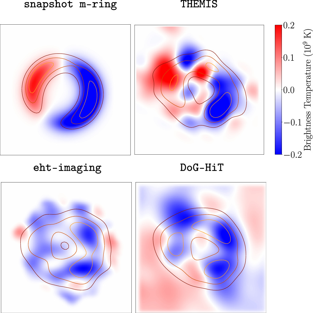
Figure 11. Circular polarimetric images of Sgr A* from the combined 2017 April 6 and 7 observations with the primary methods snapshot m-ring modeling and Themis and the validation methods eht-imaging and DoG-HiT. The posterior-average image is shown for the posterior exploration methods. Total intensity is indicated in colored linear-scale contours at 25%, 50%, and 75% of the peak brightness. The Stokes  brightness is indicated in the diverging color map, with red/blue indicating a positive/negative sign. The color-bar range is fixed for all panels.
Download figure:
Standard image High-resolution image
Figure 12. Difference of closure phases between RR* and LL* visibilities, observed on the ALMA-SMA-LMT (top) and ALMA-SMT-LMT (bottom) triangles on April 6 (squares) and April 7 (circles). Open and filled markers denote low- and high-band data, respectively. The plots follow the bottom panels of Figure 4. Predictions from the models shown in Figure 11 are also given (red and blue solid lines). They are mostly consistent with small and predominantly negative measured closure phase differences.
Download figure:
Standard image High-resolution image7. Discussion
We derive eight observational constraints from reconstructed images of Sgr A*, and these are shown in Figure 13. Since the snapshot m-ring modeling and Themis methods both provide Bayesian posterior distributions, error bars representing the 90% confidence intervals from random posterior draws are shown. The combined 90% confidence intervals from these two methods, shown in Table 6, are used in Paper VIII for theoretical interpretation. The RML imaging methods eht-imaging and DoG-HiT do not provide such distributions, but they are shown in Figure 13 as additional consistency checks from image reconstruction methods with very different methodologies. More detail on the individual methods is provided in Appendix A. We note that both posterior exploration methods treat variability differently: the snapshot m-ring modeling fits a structurally restricted ring model to individual 2-minute data snapshots, while Themis Bayesian imaging reconstructs a collection of static images from the entire 2-day data set with a noise budget accounting for variability. Despite their substantial algorithmic differences, these two methods perform best on the synthetic data tests presented in Appendix B and yield very similar results.

Figure 13. Comparisons of the measured linear and circular polarimetric quantities from the Sgr A* reconstructions across methods. For the RML imaging methods, the filled and open symbols represent the April 6 and 7 results, respectively. The gray symbols represent the 2-day averages. The error bars for the snapshot m-ring and Themis Bayesian imaging methods represent the 90% confidence range from the day-combined posterior distributions. The shaded region corresponds to the 5th to 95th percentile regions from ALMA-only linear and circular polarization light curves from Wielgus et al. (2022b). The m-ring method does not return a measurement for vnet because it fixes the value to the ALMA mean measurement before fitting. Based on their performance on the synthetic data tests and quantified distributions, the results from the snapshot m-ring and Themis methods are used for theoretical comparisons in the companion Paper VIII.
Download figure:
Standard image High-resolution imageTable 6. Polarimetric Constraints Derived from the Primary Methods Themis and Snapshot m-ring Modeling
| Observable | Snapshot m-ring | Themis | Combined |
|---|---|---|---|
| ∣mnet∣ (%) | (2.0, 3.1) | (6.5, 7.3) | (2.0, 7.3) |
| vnet (%) | ⋯ | (−0.7, 0.12) | (−0.7, 0.12) |
| 〈∣m∣〉 (%) | (24, 28) | (26, 28) | (24, 28) |
| 〈∣v∣〉 (%) | (1.4, 1.8) | (2.7, 5.5) | (0.0, 5.5) |
| ∣β1∣ | (0.11, 0.14) | (0.10, 0.13) | (0.10, 0.14) |
| ∣β2∣ | (0.20, 0.24) | (0.14, 0.17) | (0.14, 0.24) |
| ∠β2 (deg) (as observed) | (125, 137) | (142, 159) | (125, 159) |
| ∠β2 (deg) (RM derotated) | (−168, −108) | (−151, −85) | (−168, −85) |
| ∣β2∣/∣β1∣ | (1.5, 2.1) | (1.1, 1.6) | (1.1, 2.1) |
Note. These two methods each provide posteriors, from which 90% confidence regions are quoted. Derotation assumes that the median RM can be attributed to an external Faraday screen, for which a frequency of 228.1 GHz is adopted. The 〈∣v∣〉 range is treated as an upper limit. The combined constraints are used for the theoretical interpretation presented in Paper VIII.
Download table as: ASCIITypeset image
In the leftmost panels of Figure 13, the image-integrated net linear and circular polarization fractions ∣mnet∣ and vnet from the Sgr A* reconstructions are compared to ranges from interferometric-ALMA light curves treating Sgr A* as an unresolved point source from Wielgus et al. (2022a). In general, all methods are broadly consistent with ALMA ranges, although this need not necessarily have been the case. While the ranges for ALMA light curves correspond to instantaneous measurements of ∣mnet∣ and vnet, the ∣mnet∣ and vnet from our image reconstructions correspond to one or two night averages, as indicated. We note that Themis and the m-ring model do not agree on ∣mnet∣. Individual snapshot images from the m-ring method yield much higher values of ∣mnet∣. The lower ∣mnet∣ in the averaged m-ring image may be due to a combination of cancellations of time-varying structure and model misspecification issues leading to phase offsets of the fitted ∣mnet∣ (see Appendix A for details).
We also measure the image-averaged linear and circular polarization fractions 〈∣m∣〉 and 〈∣v∣〉 across the reconstructed images. For 〈∣m∣〉 in particular, we note great consistency between the two posterior exploration methods, leading to stringent constraints for theoretical models in Paper VIII. Since 〈∣v∣〉 is significantly biased upward when the S/N is poor, this quantity is interpreted as an upper limit, as in previous studies of M87* (M87* Paper IX). We recall that both 〈∣m∣〉 and 〈∣v∣〉 are resolution dependent; unlike in past studies (M87* Paper VIII; M87* Paper IX), we do not apply any blurring after image reconstruction before computing these quantities.
In the bottom panel of the third column of Figure 13, the ∠β2 measured across methods is consistently far from 0, implying more toroidal than radial EVPA patterns in the reconstructed images of Sgr A*. Accounting for a constant RM assuming an external Faraday screen, the EVPA pattern is derotated by ∼50°, leading to a large ∠β2 of the opposite sign (the faded points in the ∠β2 panel). While the RM correction flips the handedness of the EVPA pattern (see Figures 8–9) and thus poses a significant systematic for comparisons to theoretical models, the EVPA patterns across methods remain very toroidal (∠β2 is closer to ±180° than 0°; Palumbo et al. 2020).
8. Conclusions and Summary
We presented the linear and circular polarimetric imaging of the EHT 2017 April 6 and 7 observations of our Galactic center black hole Sgr A* on event horizon scales at 230 GHz. Our analysis builds on the total-intensity ring morphology results presented in Papers I–VI and made use of the leakage calibration derived in M87* Paper VII. We employed four distinct methods in the polarimetric analysis: two posterior exploration (one Bayesian imaging and one snapshot modeling) methods for primary analysis and two RML imaging methods for validation. All methods were tested on synthetic data designed to mimic specific polarimetric characteristics of Sgr A*. When applied to the EHT Sgr A* data, all methods showed that the emission ring is highly polarized, with a peak fractional linear polarization of ∼40% in the western region of the ring. While the detailed spatial distribution of the linear polarization along the ring is uncertain owing to the intrinsic variability of Sgr A* (as was the case for the total-intensity results), we observed a coherent spiraling polarization structure across a large portion of the ring that is robust to methodological choices. The circular polarization reconstructions from the posterior exploration methods, which performed best on the synthetic tests, prefer a dipole structure along the ring, with negative circular polarization emission on the west of the ring (also recovered by the RML imaging methods) and positive emission mostly constrained to the northeast, with peak absolute values that are 5%–10% of the Stokes  emission in the same locations. Although both our posterior exploration methods reproduce a dipole along the ring, we deem the circular polarization structure more uncertain given the stronger disagreement between methods compared to the linear polarization reconstructions.
The resolution and sensitivity of the EHT have provided horizon-scale polarimetric images of Sgr A*, enabling for the first time a reconstruction of the magnetic field geometry in the vicinity of our Galactic center supermassive black hole's event horizon. A discussion of the physical interpretation of these results is presented in Paper VIII.
Acknowledgments
The Event Horizon Telescope Collaboration thanks the following organizations and programs: the Academia Sinica; the Academy of Finland (projects 274477, 284495, 312496, 315721); the Agencia Nacional de Investigación y Desarrollo (ANID), Chile via NCN19058 (TITANs), Fondecyt 1221421, and BASAL FB210003; the Alexander von Humboldt Stiftung; an Alfred P. Sloan Research Fellowship; Allegro, the European ALMA Regional Centre node in the Netherlands, the NL astronomy research network NOVA and the astronomy institutes of the University of Amsterdam, Leiden University, and Radboud University; the ALMA North America Development Fund; the Astrophysics and High Energy Physics program by MCIN (with funding from European Union NextGenerationEU, PRTR-C17I1); the Black Hole Initiative, which is funded by grants from the John Templeton Foundation (60477, 61497, 62286) and the Gordon and Betty Moore Foundation (grant GBMF-8273)—although the opinions expressed in this work are those of the author and do not necessarily reflect the views of these Foundations; the Brinson Foundation; "la Caixa" Foundation (ID 100010434) through fellowship codes LCF/BQ/DI22/11940027 and LCF/BQ/DI22/11940030; Chandra DD7-18089X and TM6-17006X; the China Scholarship Council; the China Postdoctoral Science Foundation fellowships (2020M671266, 2022M712084); Consejo Nacional de Humanidades, Ciencia y Tecnología (CONAHCYT, Mexico, projects U0004-246083, U0004-259839, F0003-272050, M0037-279006, F0003-281692, 104497, 275201, 263356); the Colfuturo Scholarship; the Consejería de Economía, Conocimiento, Empresas y Universidad of the Junta de Andalucía (grant P18-FR-1769); the Consejo Superior de Investigaciones Científicas (grant 2019AEP112); the Delaney Family via the Delaney Family John A. Wheeler Chair at Perimeter Institute; Dirección General de Asuntos del Personal Acadëmico-Universidad Nacional Autónoma de Mèxico (DGAPA-UNAM, projects IN112820 and IN108324); the Dutch Organization for Scientific Research (NWO) for the VICI award (grant 639.043.513), the grant OCENW.KLEIN.113, and the Dutch Black Hole Consortium (with project No. NWA 1292.19.202) of the research program the National Science Agenda; the Dutch National Supercomputers, Cartesius and Snellius (NWO grant 2021.013); the EACOA Fellowship awarded by the East Asia Core Observatories Association, which consists of the Academia Sinica Institute of Astronomy and Astrophysics, the National Astronomical Observatory of Japan, Center for Astronomical Mega-Science, Chinese Academy of Sciences, and the Korea Astronomy and Space Science Institute; the European Research Council (ERC) Synergy grant "BlackHoleCam: Imaging the Event Horizon of Black Holes"' (grant 610058); the European Union's Horizon 2020 research and innovation program under grant agreements RadioNet (No. 730562) and M2FINDERS (No. 101018682); the Horizon ERC Grants 2021 program under grant agreement No. 101040021; the European Research Council for advanced grant "JETSET: Launching, propagation and emission of relativistic jets from binary mergers and across mass scales" (grant No. 884631); the FAPESP (Fundaç ao de Amparo á Pesquisa do Estado de S ao Paulo) under grant 2021/01183-8; the Fondo CAS-ANID folio CAS220010; the Generalitat Valenciana (grants APOSTD/2018/177 and ASFAE/2022/018) and GenT Program (project CIDEGENT/2018/021); the Gordon and Betty Moore Foundation (GBMF-3561, GBMF-5278, GBMF-10423); the Institute for Advanced Study; the Istituto Nazionale di Fisica Nucleare (INFN) sezione di Napoli, iniziative specifiche TEONGRAV; the International Max Planck Research School for Astronomy and Astrophysics at the Universities of Bonn and Cologne; DFG research grant "Jet physics on horizon scales and beyond" (grant No. 443220636); Joint Columbia/Flatiron Postdoctoral Fellowship (research at the Flatiron Institute is supported by the Simons Foundation); the Japan Ministry of Education, Culture, Sports, Science and Technology (MEXT; grant JPMXP1020200109); the Japan Society for the Promotion of Science (JSPS) grant-in-aid for JSPS Research Fellowship (JP17J08829); the Joint Institute for Computational Fundamental Science, Japan; the Key Research Program of Frontier Sciences, Chinese Academy of Sciences (CAS, grants QYZDJ-SSW-SLH057, QYZDJ-SSW-SYS008, ZDBS-LY-SLH011); the Leverhulme Trust Early Career Research Fellowship; the Max-Planck-Gesellschaft (MPG); the Max Planck Partner Group of the MPG and the CAS; the MEXT/JSPS KAKENHI (grants 18KK0090, JP21H01137, JP18H03721, JP18K13594, 18K03709, JP19K14761, 18H01245, 25120007, 23K03453); the MICINN Research Projects PID2019-108995GB-C22, PID2022-140888NB-C22; the MIT International Science and Technology Initiatives (MISTI) Funds; the Ministry of Science and Technology (MOST) of Taiwan (103-2119-M-001-010-MY2, 105-2112-M-001-025-MY3, 105-2119-M-001-042, 106-2112-M-001-011, 106-2119-M-001-013, 106-2119-M-001-027, 106-2923-M-001-005, 107-2119-M-001-017, 107-2119-M-001-020, 107-2119-M-001-041, 107-2119-M-110-005, 107-2923-M-001-009, 108-2112-M-001-048, 108-2112-M-001-051, 108-2923-M-001-002, 109-2112-M-001-025, 109-2124-M-001-005, 109-2923-M-001-001, 110-2112-M-003-007-MY2, 110-2112-M-001-033, 110-2124-M-001-007, and 110-2923-M-001-001); the Ministry of Education (MoE) of Taiwan Yushan Young Scholar Program; the Physics Division, National Center for Theoretical Sciences of Taiwan; the National Aeronautics and Space Administration (NASA, Fermi Guest Investigator grant 80NSSC20K1567, NASA Astrophysics Theory Program grant 80NSSC20K0527, NASA NuSTAR award 80NSSC20K0645); NASA Hubble Fellowship grants HST-HF2-51431.001-A, HST-HF2-51482.001-A awarded by the Space Telescope Science Institute, which is operated by the Association of Universities for Research in Astronomy, Inc., for NASA, under contract NAS5-26555; the National Institute of Natural Sciences (NINS) of Japan; the National Key Research and Development Program of China (grant 2016YFA0400704, 2017YFA0402703, 2016YFA0400702); the National Science and Technology Council (NSTC, grants NSTC 111-2112-M-001-041, NSTC 111-2124-M-001-005, NSTC 112-2124-M-001-014); the US National Science Foundation (NSF, grants AST-0096454, AST-0352953, AST-0521233, AST-0705062, AST-0905844, AST-0922984, AST-1126433, OIA-1126433, AST-1140030, DGE-1144085, AST-1207704, AST-1207730, AST-1207752, MRI-1228509, OPP-1248097, AST-1310896, AST-1440254, AST-1555365, AST-1614868, AST-1615796, AST-1715061, AST-1716327, AST- 1726637, OISE-1743747, AST-1743747, AST-1816420, AST-1952099, AST-1935980, AST-2034306, AST-2205908, AST-2307887); NSF Astronomy and Astrophysics Postdoctoral Fellowship (AST-1903847); the Natural Science Foundation of China (grants 11650110427, 10625314, 11721303, 11725312, 11873028, 11933007, 11991052, 11991053, 12192220, 12192223, 12273022, 12325302, 12303021); the Natural Sciences and Engineering Research Council of Canada (NSERC, including a Discovery grant and the NSERC Alexander Graham Bell Canada Graduate Scholarships-Doctoral Program); the National Youth Thousand Talents Program of China; the National Research Foundation of Korea (the Global PhD Fellowship grant: grants NRF-2015H1A2A1033752, the Korea Research Fellowship Program: NRF-2015H1D3A1066561, Brain Pool Program: 2019H1D3A1A01102564, Basic Research Support grant 2019R1F1A1059721, 2021R1A6A3A01086420, 2022R1C1C1005255, 2022R1F1A1075115); Netherlands Research School for Astronomy (NOVA) Virtual Institute of Accretion (VIA) postdoctoral fellowships; NOIRLab, which is managed by the Association of Universities for Research in Astronomy (AURA) under a cooperative agreement with the National Science Foundation; Onsala Space Observatory (OSO) national infrastructure, for the provisioning of its facilities/observational support (OSO receives funding through the Swedish Research Council under grant 2017-00648); the Perimeter Institute for Theoretical Physics (research at Perimeter Institute is supported by the Government of Canada through the Department of Innovation, Science and Economic Development and by the Province of Ontario through the Ministry of Research, Innovation and Science); the Princeton Gravity Initiative; the Spanish Ministerio de Ciencia e Innovación (grants PGC2018-098915-B-C21, AYA2016-80889-P, PID2019-108995GB-C21, PID2020-117404GB-C21); the University of Pretoria for financial aid in the provision of the new Cluster Server nodes and SuperMicro (USA) for a SEEDING grant approved toward these nodes in 2020; the Shanghai Municipality orientation program of basic research for international scientists (grant no. 22JC1410600); the Shanghai Pilot Program for Basic Research, Chinese Academy of Science, Shanghai Branch (JCYJ-SHFY-2021-013); the State Agency for Research of the Spanish MCIU through the "Center of Excellence Severo Ochoa" award for the Instituto de Astrofísica de Andalucía (SEV-2017-0709); the Spanish Ministry for Science and Innovation grant CEX2021-001131-S funded by MCIN/AEI/10.13039/501100011033; the Spinoza Prize SPI 78-409; the South African Research Chairs Initiative, through the South African Radio Astronomy Observatory (SARAO, grant ID 77948), which is a facility of the National Research Foundation (NRF), an agency of the Department of Science and Innovation (DSI) of South Africa; the Toray Science Foundation; the Swedish Research Council (VR); the UK Science and Technology Facilities Council (grant no. ST/X508329/1); the US Department of Energy (USDOE) through the Los Alamos National Laboratory (operated by Triad National Security, LLC, for the National Nuclear Security Administration of the USDOE, contract 89233218CNA000001); and the YCAA Prize Postdoctoral Fellowship.
We thank the staff at the participating observatories, correlation centers, and institutions for their enthusiastic support. This paper makes use of the following ALMA data: ADS/JAO.ALMA#2016.1.01154.V. ALMA is a partnership of the European Southern Observatory (ESO; Europe, representing its member states), NSF, and National Institutes of Natural Sciences of Japan, together with National Research Council (Canada), Ministry of Science and Technology (MOST; Taiwan), Academia Sinica Institute of Astronomy and Astrophysics (ASIAA; Taiwan), and Korea Astronomy and Space Science Institute (KASI; Republic of Korea), in cooperation with the Republic of Chile. The Joint ALMA Observatory is operated by ESO, Associated Universities, Inc. (AUI)/NRAO, and the National Astronomical Observatory of Japan (NAOJ). The NRAO is a facility of the NSF operated under cooperative agreement by AUI. This research used resources of the Oak Ridge Leadership Computing Facility at the Oak Ridge National Laboratory, which is supported by the Office of Science of the U.S. Department of Energy under contract No. DE-AC05-00OR22725; the ASTROVIVES FEDER infrastructure, with project code IDIFEDER-2021-086; and the computing cluster of Shanghai VLBI correlator supported by the Special Fund for Astronomy from the Ministry of Finance in China. We also thank the Center for Computational Astrophysics, National Astronomical Observatory of Japan. This work was supported by FAPESP (Fundacao de Amparo a Pesquisa do Estado de Sao Paulo) under grant 2021/01183-8.
APEX is a collaboration between the Max-Planck-Institut für Radioastronomie (Germany), ESO, and the Onsala Space Observatory (Sweden). The SMA is a joint project between the SAO and ASIAA and is funded by the Smithsonian Institution and the Academia Sinica. The JCMT is operated by the East Asian Observatory on behalf of the NAOJ, ASIAA, and KASI, as well as the Ministry of Finance of China, Chinese Academy of Sciences, and the National Key Research and Development Program (No. 2017YFA0402700) of China and Natural Science Foundation of China grant 11873028. Additional funding support for the JCMT is provided by the Science and Technologies Facility Council (UK) and participating universities in the UK and Canada. The LMT is a project operated by the Instituto Nacional de Astrófisica, Óptica, y Electrónica (Mexico) and the University of Massachusetts at Amherst (USA). The IRAM 30 m telescope on Pico Veleta, Spain is operated by IRAM and supported by CNRS (Centre National de la Recherche Scientifique, France), MPG (Max-Planck-Gesellschaft, Germany), and IGN (Instituto Geográfico Nacional, Spain). The SMT is operated by the Arizona Radio Observatory, a part of the Steward Observatory of the University of Arizona, with financial support of operations from the State of Arizona and financial support for instrumentation development from the NSF. Support for SPT participation in the EHT is provided by the National Science Foundation through award OPP-1852617 to the University of Chicago. Partial support is also provided by the Kavli Institute of Cosmological Physics at the University of Chicago. The SPT hydrogen maser was provided on loan from the GLT, courtesy of ASIAA.
This work used the Extreme Science and Engineering Discovery Environment (XSEDE), supported by NSF grant ACI-1548562, and CyVerse, supported by NSF grants DBI-0735191, DBI-1265383, and DBI-1743442. XSEDE Stampede2 resource at TACC was allocated through TG-AST170024 and TG-AST080026N. XSEDE JetStream resource at PTI and TACC was allocated through AST170028. This research is part of the Frontera computing project at the Texas Advanced Computing Center through the Frontera Large-Scale Community Partnerships allocation AST20023. Frontera is made possible by National Science Foundation award OAC-1818253. This research was done using services provided by the OSG Consortium (Pordes et al. 2007; Sfiligoi et al. 2009) supported by the National Science Foundation award Nos. 2030508 and 1836650. Additional work used ABACUS2.0, which is part of the eScience center at Southern Denmark University, and the Kultrun Astronomy Hybrid Cluster (projects Conicyt Programa de Astronomia Fondo Quimal QUIMAL170001, Conicyt PIA ACT172033, Fondecyt Iniciacion 11170268, Quimal 220002). Simulations were also performed on the SuperMUC cluster at the LRZ in Garching, on the LOEWE cluster in CSC in Frankfurt, on the HazelHen cluster at the HLRS in Stuttgart, and on the Pi2.0 and Siyuan Mark-I at Shanghai Jiao Tong University. The computer resources of the Finnish IT Center for Science (CSC) and the Finnish Computing Competence Infrastructure (FCCI) project are acknowledged. This research was enabled in part by support provided by Compute Ontario (http://computeontario.ca), Calcul Quebec (http://www.calculquebec.ca), and Compute Canada (http://www.computecanada.ca).
The EHTC has received generous donations of FPGA chips from Xilinx Inc., under the Xilinx University Program. The EHTC has benefited from technology shared under open-source license by the Collaboration for Astronomy Signal Processing and Electronics Research (CASPER). The EHT project is grateful to T4Science and Microsemi for their assistance with hydrogen masers. This research has made use of NASA's Astrophysics Data System. We gratefully acknowledge the support provided by the extended staff of the ALMA, from the inception of the ALMA Phasing Project through the observational campaigns of 2017 and 2018. We would like to thank A. Deller and W. Brisken for EHT-specific support with the use of DiFX. We thank Martin Shepherd for the addition of extra features in the Difmap software that were used for the CLEAN imaging results presented in this paper. We acknowledge the significance that Maunakea, where the SMA and JCMT EHT stations are located, has for the indigenous Hawaiian people.
Facilities: EHT - , ALMA - Atacama Large Millimeter Array, APEX - Atacama Pathfinder Experiment, IRAM:30m - Institute de Radioastronomie Millimetrique 30 meter telescope, JCMT - James Clerk Maxwell Telescope, LMT - , SMA - SubMillimeter Array, ARO:SMT - , SPT - South Pole Telescope.
Software: DiFX (Deller et al. 2011), CALC, PolConvert (Martí-Vidal et al. 2016), HOPS (Whitney et al. 2004), EHT-HOPS Pipeline (Blackburn et al. 2019), CASA (McMullin et al. 2007), rPICARD (Janssen et al. 2018, 2019), eht-imaging (Chael et al. 2016), DoG-HiT (Müller & Lobanov 2022), Themis (Broderick et al. 2020c), Numpy (Harris et al. 2020), Scipy (Jones et al. 2001), Pandas (McKinney 2010), Astropy (The Astropy Collaboration et al. 2013, 2018), Jupyter (Kluyver et al. 2016), Matplotlib (Hunter 2007).
Appendix A: Method Details
A.1. M-ring Snapshot Modeling
In geometric modeling, the source structure is described by a low-dimensional model that is fit to the observational data. Geometric modeling is generally fast, since operations like the Fourier transform and gradient computation can be performed analytically. The geometric model parameters often directly correspond to source structure parameters of interest (e.g., ring diameter, thickness, and asymmetry). On the other hand, geometric modeling suffers from the issue of model misspecification: a geometric model typically does not capture all underlying image features, even if the angular resolution is limited. However, by restricting the image-domain parameter space, geometric modeling can constrain the low-order image structure in regimes where imaging methods encounter difficulties because of the many degrees of freedom (image pixel values). Geometric modeling is therefore particularly useful for data sets with sparse baseline coverage and/or low-S/N data.
In the analysis of EHT data, geometric modeling has been used to constrain the event horizon scale structure of M87* in full Stokes (M87* Paper VI; Wielgus et al. 2022a; M87* Paper IX; Roelofs et al. 2023) and the event horizon scale structure of Sgr A* in total intensity (Paper IV). For EHT data of Sgr A*, snapshot geometric modeling provides a way to mitigate rapid source variability. In snapshot modeling, the data set is split up into short (2-minute) snapshots fitted independently with the geometric model. The snapshot results are then combined using a Bayesian hierarchical model in order to obtain a posterior for the average image structure; see Paper IV for details. In this work, we use snapshot geometric modeling in combination with this Bayesian averaging procedure to constrain the structure of Sgr A* in full Stokes.
Like in Paper IV and M87* Paper IX, our geometric model of choice is the m-ring model. The m-ring model parameterizes the image-domain structure as a ring with diameter d, width (FWHM) α, and an azimuthal structure set by Fourier modes in total intensity, linear polarization, and circular polarization (Johnson et al. 2020; Paper IV; Roelofs et al. 2023). In total-intensity and polar image coordinates, the m-ring has the form

Here δ is the Dirac delta distribution, and the  are the Fourier coefficients setting the azimuthal structure. We have set
  so that F > 0 gives the total flux density of the ring. The higher the m-ring order
  , the more complex azimuthal structures can be modeled. A finite thickness is introduced by blurring the m-ring using a circular Gaussian kernel with FWHM α. Unlike Paper IV, we do not add a Gaussian floor component to our m-ring model.
The linear polarization structure  and the circular polarization structure
  are parameterized analogously, with the azimuthal structure set by
  and
and  , respectively. Since the total-intensity and circular polarization structures are real-valued,
  and
and  . In contrast, the linear polarization structures are complex-valued, and thus we fit
  and
and  independently. The m-ring orders in linear and circular polarization are indicated with
  and
and  , respectively. The net linear and circular polarization fractions are given by
  and
and  , respectively. The polarization structure is thus parameterized in fractional terms and can be converted to polarized intensities via multiplication by F in Equation (A1).
Before fitting the m-ring model in full Stokes to Sgr A*, we preprocess the data by adding 2% fractional systematic noise to the visibilities, deblurring to mitigate the effects of interstellar scattering, leakage-calibrating, and light-curve-normalizing the data and splitting the data into 2-minute snapshots. We only fit to snapshots with data on at least 10 baselines and with a coherent integration time of at least 60 s. Since each snapshot is fit independently, there is no need for the introduction of an additional noise budget representing intrinsic source variability. Following Roelofs et al. (2023), we first fit the total-intensity and linear polarization structure to parallel-hand closure phases, closure amplitudes, and the visibility-domain fractional linear polarization  . These data products are invariant to complex gain corruptions except for an R/L gain ratio dependence of
  . We then fix the linear polarization parameters to the MAP estimates and fit the total-intensity and circular polarization structure either to the separate parallel-hand (RR* and LL*) closure phases and closure amplitudes or to the RR*/LL* visibility ratios. Since the closure products cannot constrain vnet, we fix vnet to the mean value from the ALMA light curve (−1.14%). The RR*/LL* data product is sensitive to residual R/L gain ratios that may be present in our data (see Roelofs et al. 2023, for details). Erring on the conservative side, we therefore present our closure-only fits in Figure 11 and comment on our RR*/LL* fits below. We set
  ,
,  , and
, and  for all fits presented in this work. These are the maximum m-orders that produce reasonable results based on performance on synthetic data tests, an investigation of the Bayesian evidence (see also Paper IV), and the stability of the fit results as the m-orders are increased. All fitting is done with eht-imaging, using dynesty (Speagle 2020) for posterior exploration.
Figure 14 shows 1σ posterior ranges for snapshots on all days and bands, for a few polarization parameters of interest. The Bayesian average posterior range is also indicated by the green bands. ∣mnet∣ ranges between ∼2.5% and ∼15% for the individual snapshots, and the Bayesian average is at the lower end of this range. The Bayesian averaging procedure approximately performs a complex average on complex parameters, so that the resulting absolute values are usually lower than the individual snapshots because of angular variations (in this case related to the net EVPA). In addition, we find that the m-ring model does not fit the zero-baseline  phase well for all snapshots. These zero-baseline phase offsets result in a larger spread on the fitted ∣mnet∣ phase across snapshots than what is expected from the zero-baseline measurements, leading to a lower amplitude after Bayesian averaging. The phase offsets are likely caused by a combination of model misspecification and S/N differences between baselines. High-S/N data points on intermediate baselines are fit well, while lower-S/N points on short baselines are fit more poorly. The
  S/N on short baselines is low because of the low total polarization fraction, and the differences are amplified by the addition of systematic noise (which is a fixed fraction of the visibility amplitudes).
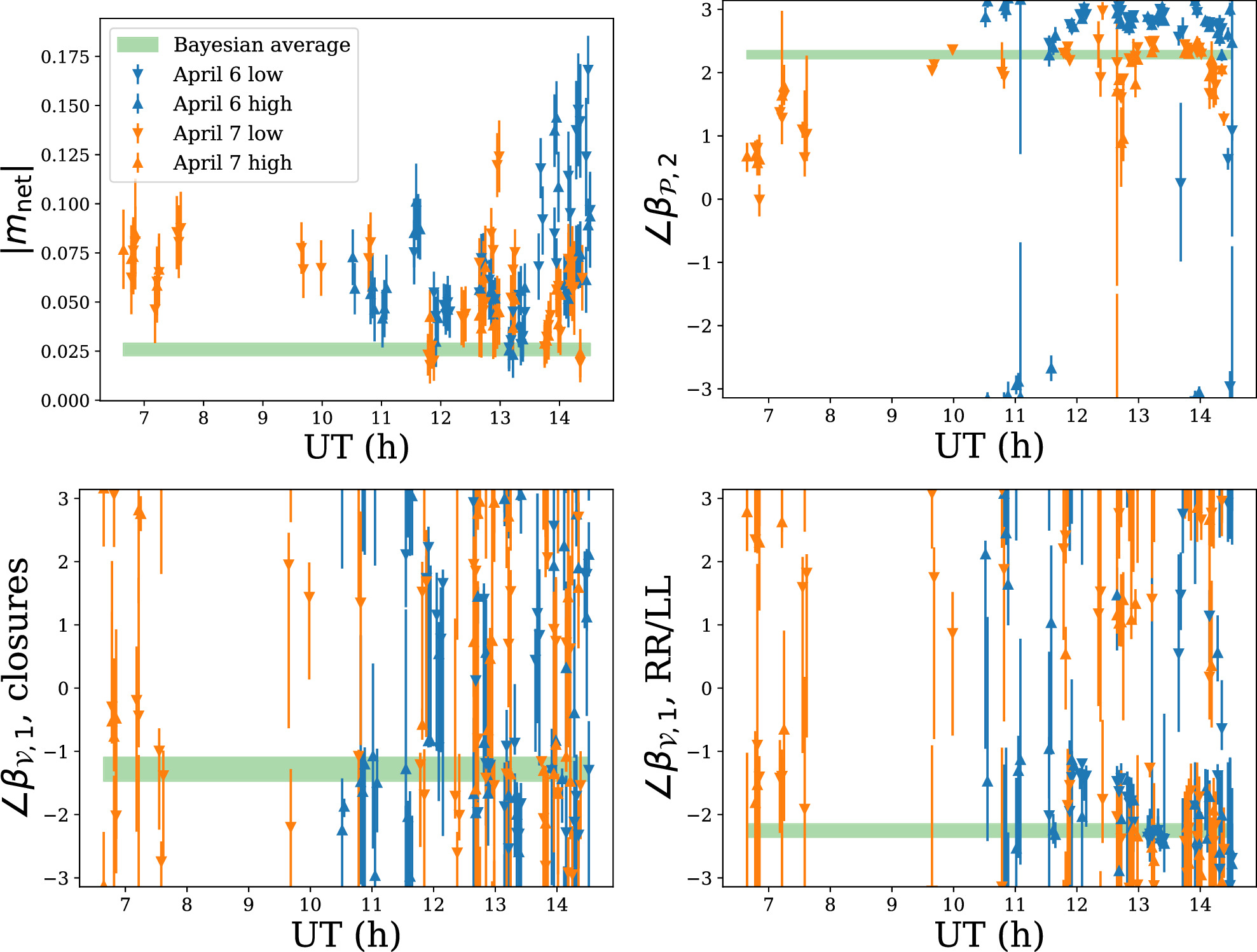
Figure 14. Snapshot m-ring posteriors (1σ ranges) for linear polarization parameters ∣mnet∣ and  (top row) and circular polarization parameter
  (i.e., the first-order Stokes
  orientation) for fits to closure quantities and RR/LL visibility ratios (bottom row). The green bands indicate the 1σ ranges for the time and band-averaged structure computed using our Bayesian averaging procedure. Since this procedure approximately produces a complex average, the resulting amplitudes of complex quantities like ∣mnet∣ tend to be lower than those of individual snapshots.
Download figure:
Standard image High-resolution image
 is relatively stable between snapshots, with a systematic offset between the 2 days.
  (bottom row), which is the first-order orientation of the circular polarization emission, is relatively unconstrained for individual snapshots when fitting only to the parallel-hand closure products (bottom left panel), although the Bayesian averaging procedure indicates a preferred orientation that is roughly consistent with other methods (Figure 11). A clearer preference for an approximately northwest–southeast asymmetry is indicated by the RR*/LL* fits (bottom right panel). Since the
  Bayesian average of the RR*/LL* and closure fits are formally inconsistent at the 1σ level (although they are within a quadrant of each other) and the RR*/LL* fits may be affected by unknown residual R/L gain ratios, we only use the closure fits for our reported parameter ranges and theoretical interpretation (e.g., Table 6, Figure 13).
A.2. Themis
The Themis package is a Bayesian framework designed for the analysis of EHT data (Broderick et al. 2020c). It provides a well-tested, uniform set of independent tools for addressing station-based and astrophysical systematics, including complex gain reconstruction, polarimetric leakage estimation (D-terms), and interstellar scattering models. Themis provides a number of posterior sampling methods, for which the most common output is a Markov Chain Monte Carlo (MCMC) chain that supports subsequent Bayesian interpretation. In the case of imaging models (Broderick et al. 2020), these posteriors permit Bayesian interpretations of image features.
Themis fits the complex parallel-hand and cross-hand visibilities. Prior to fitting, the data are calibrated as described in Section 2, scan-averaged, and normalized by the Stokes  light curve, as described in Papers III and IV. The calibrator estimates of the complex gains and D-terms are applied, and thus Themis estimates are additional corrections to each. High- and low-band data from April 6 and 7 are fit simultaneously, ensuring that the underlying assumptions of the variability reconstruction are satisfied (see Broderick et al. 2022).
The polarimetric image model in Themis is based on the Stokes  imaging model presented in Broderick et al. (2020) and previously used in M87* Paper VII and M87* Paper IX. Four fields are simultaneously reconstructed:
- 1.the Stokes map;
- 2.the total polarization fraction;
- 3.the linear polarization EVPA; and
- 4.the fraction of polarized flux associated with Stokes,


each of which is represented by a fixed number of control points located on a rectilinear raster with priors as stated in M87* Paper VII and M87* Paper IX, between which the image is interpolated via a bicubic spline; see Broderick et al. (2020). The field of view along the two axes of the raster and the raster orientation are model parameters and permitted to vary. Diffractive scattering is applied directly to the associated visibilities, assuming the scattering model in Johnson et al. (2018), with the default scattering parameters from Issaoun et al. (2021). Complex gains are reconstructed independently by scan as described in Paper III. Polarization leakage is solved for using the Sgr A* data alone, with flat priors on the interval (−1, 1) on real and imaginary components of the left and right D-terms for each station.
The intrahour variability of Sgr A* is mitigated via explicit modeling of the additional fluctuations about the mean image as described in Broderick et al. (2022), modified as described in Section 4.1.2. Simultaneously, additional contributions to the excess uncertainty budget are allocated to account for the refractive scattering noise and systematic (e.g., nonclosing) errors, as described in Paper IV. With the exception of the parallel-hand/cross-hand variance, which is held fixed at the value implied by the empirically estimated power spectra, all other parameters in the uncertainty model are permitted to vary during image reconstruction (see Papers III and IV for details).
To ensure efficient sampling of the posterior, we use the differential even–odd parallel tempering scheme with each tempering level explored via the Hamiltonian Monte Carlo NUTS algorithm implemented by the Stan package (Carpenter et al. 2017; Syed et al. 2019). This sampler has been demonstrated to effectively capture multimodal posteriors (see, e.g., M87* Paper VII; Paper IV). Chain convergence is assessed by visual inspection of parameter traces and quantitative chain statistics, including the integrated autocorrelation time, split- , and parameter rank distributions (Vehtari et al. 2019), and typically requires ∼105 MCMC steps. The number of tempering levels is chosen to ensure efficient communication between the highest- and lowest-temperature levels, here typically 65 due to the complicated nature of the model.
Three key additional systematic uncertainties explored by the Themis polarimetric image posterior are the impact of leakage corrections, station gains, and the underlying Stokes  image. D-term corrections relative to the calibrator-implied values from the Themis posterior (obtained from the Sgr A* data alone) are shown in Figure 15 in comparison to the sizes implied by Themis polarimetric reconstructions of the April 11 M87* data (M87* Paper VII). Most corrections are consistent with being small (<10%), with the large uncertainties (>10%) at PV and SMA indicative of the poor parallactic angle coverage of Sgr A* at those stations. Regardless, the images are robust to even large D-terms, indicating that the final polarimetric structure is robust to the leakage calibration. The minimal impact of D-terms on polarimetric structure is also consistent with the findings in Appendix H of M87* Paper VII assessing their effect on polarimetric images of the static M87* black hole. Inspection of the complex gain reconstructions indicates only small deviations from the calibrator-implied gains applied before analysis: for ALMA, APEX, and SMA the gain amplitude corrections are of order 0.2%; for SMT and PV they are of order 5%; and for LMT and SPT they are roughly 10%. Sgr A* MCMC chains were initialized using the Stokes
  image from Paper III to decrease time to MCMC convergence. For the simulated data tests the MCMC chains were initialized both with Stokes
  images and with a diffuse Gaussian of approximately the size implied by second-moment visibility analyses, with both cases converging to the same posteriors, providing confidence that the particular initialization is unimportant. For Sgr A*, multiple qualitatively similar modes are found, differing subtly in the distribution of flux about the ring and the structure of the extended diffuse emission.

Figure 15. Posteriors of the leakage term corrections, applied after calibration with the 2017 M87* D-terms, obtained by Themis via fitting to the 2017 April 6 and 7 data on Sgr A* alone (i.e., without considering other calibrators). Contours show 1σ, 2σ, and 3σ cumulative regions. For comparison, the 2σ uncertainties from the Themis 2017 M87* values are indicated by the black error bars. The substantially weaker constraints on the IRAM 30 m (PV) and SMA D-terms are direct consequences of the relatively poorer parallactic angle coverage during the Sgr A* observations. Similarly, because M87* is not visible from the south pole, the SPT has no comparison point.
Download figure:
Standard image High-resolution imageA.3. Eht-imaging
The eht-imaging (Chael et al. 2016, 2018) package reconstructs polarimetric images via RML. eht-imaging solves for an image X by minimizing an objective function via gradient descent. The minimized objective function J( X ) is a weighted sum of data reduced χ2 log-likelihood terms and regularizer terms that favor or penalize specific image properties:

RML imaging thus requires optimizing the "hyperparameter" weights αi and βj in Equation (A2) to recover high-fidelity images. Here we describe the data terms and regularizers we use for polarimetric imaging.
For polarized image reconstructions, we follow the method laid out in Chael et al. (2016) and Appendix C of M87* Paper VII. The only major difference with the M87* polarimetric analysis is the exclusion of the D-term solving steps, because the Sgr A* data are leakage corrected following the M87* (and calibrator) analysis. We start with leakage-calibrated data that have had the overall time-dependent station amplitude and phase gains calibrated using the static average image from Paper III. The data are time averaged to 120 s, a systematic noise budget of 5% is applied, and a noise budget is added in quadrature to the uncertainties on the visibilities following the variability studies discussed in Section 4.1. We then reconstruct a Stokes  image using top-set parameters for eht-imaging developed in Paper III. We fix the image field of view at 150 μas and solve for the intensities on a grid of 64 × 64 pixels. We next (re-)self-calibrate the station amplitude and phase gains (assuming GR
= GL
) to our final Stokes
image using top-set parameters for eht-imaging developed in Paper III. We fix the image field of view at 150 μas and solve for the intensities on a grid of 64 × 64 pixels. We next (re-)self-calibrate the station amplitude and phase gains (assuming GR
= GL
) to our final Stokes  image. Using this image as the prior for polarimetric imaging, we then reconstruct linear and circular polarization images separately.
For linear polarization image reconstruction, the objective function in Equation (A2) includes two log-likelihood χ2 terms: one computed using the RL* polarimetric visibility  , and one using the visibility-domain polarimetric ratio
  .
.  is immune to most residual station gain errors left over from Stokes
  imaging except for R/L gain ratio, while
  is not. We use two regularizers for polarized flux density: the Holdaway–Wardle (Holdaway & Wardle 1990) regularizer SHW (Equation (13) of Chael et al. 2016) prefers image pixels that take a value less than
  (the theoretical maximum polarization for synchrotron radiation), and the total variation (TV) regularizer STV (Rudin et al. 1992) penalizes large pixel-to-pixel image gradients in both the real and imaginary parts of the complex polarization brightness distribution (Equation (15) of Chael et al. 2016). The linear polarization objective function is thus

The relative weighting between the data constraints and the regularizer terms is set by the four hyperparameters αP
, αm
, βHW, and βTV. We solve for the polarized flux distribution that minimizes Equation (A3) parameterized by the fractional polarization m and EVPA ξ in each pixel. The Stokes  image is fixed in the polarimetric imaging step and defines the region where polarimetric flux is allowed. We restart the gradient descent process several times, using the output of the previous round of imaging blurred by a 20 μas Gaussian kernel as the new initial point and iterating through imaging rounds by increasing the weights on
  and
and  . We keep the underlying data and gains fixed.
For imaging Stokes  , eht-imaging again fixes the Stokes
  image and solves for the fractional circular polarization
  in each pixel by fitting to self-calibrated
  visibilities. The circular polarization fraction is limited to the range
  by means of a change of variables between the pixel fractional polarization and the quantity solved for in gradient descent. The circular polarization objective function includes a total variation regularizer on the
  map and an ℓ1 sparsity regularizer (e.g., Akiyama et al. 2017), both of which take the same form as in total-intensity imaging (Chael et al. 2016). We again image
  in multiple rounds and perform iterative self-calibration, this time solving for right and left complex gains independently to account for relative polarimetric gain offsets. The D-terms are kept fixed during Stokes
  imaging.
A.4. DoG-HiT
The DoG-HiT procedure consists of two steps. In the first step we utilize the DoG-HiT algorithm (Müller & Lobanov 2022) to approximate a static total-intensity image and derive the multiresolution support (the set of statistically significant wavelet coefficients). In the second step, we utilize this prior information for the multiresolution support imaging strategy described in Müller & Lobanov (2023b) to add linear polarimetry and solve for the dynamics.
DoG-HiT models the image by a set of multiscalar basis functions (Müller & Lobanov 2022). The matrix containing all basis functions is commonly referred to as a dictionary, and we denote it as Γ for the rest of this discussion. The total-intensity map
X
is defined as  , where
  is the array of wavelet coefficients. The scalar widths and angular orientations of the wavelets are selected based on the (u, v) coverage, such that they separate the image structural features that are measured (covered by observations) and those that are mainly sensitive to the gaps in the (u, v) coverage. To achieve this goal, we developed special dictionaries of wavelets, or differences of elliptical Bessel functions and differences of elliptical Gaussian functions; see Müller & Lobanov (2023a) for more details. We use a sparsity-promoting regularization formalism that is analogous to Equation (A2) except that the data products being fit are closure phases and closure amplitudes that are constructed from the Stokes visibilities (
 ,
,  ), and we solve for the wavelet coefficients rather than the image:

where α is the regularization parameter and Rflux is a total flux constraint with a compact flux density f. In this framework, DoG-HiT reconstruction attempts to recover a total-intensity image while minimizing user-based choices, i.e., by using only data terms for the static total-intensity image that are robust against the self-calibration, and a data-driven choice of the regularization term. It has been demonstrated that EHT data are constraining enough for closure-only imaging of the total-intensity image (e.g., Chael et al. 2018; M87* Paper IV; Paper III; Müller et al. 2023).
In a second step, we address the dynamics and the polarimetry. During the fitting of the static DoG-HiT (Stokes  ) model to the observed visibilities, wavelets that are sensitive primarily to spatial scales associated with gaps in the (u,v) coverage have their coefficients suppressed. This prior information is used for the reconstruction of polarimetric and time-variable data sets by a constrained minimization procedure, i.e., we fit the full Stokes polarimetric visibilities independently for every frame but only vary the coefficients in the multiresolution support (Müller & Lobanov 2023b), by minimizing
  and
and  for every snapshot.
For the Stokes  static analysis of the time-variable source Sgr A*, we use the fiducial average image from the total-intensity analysis (Paper III) as an initial guess, self-calibrate the data set to this model, add systematic noise at a level of 2% at every baseline, and calculate the multiresolution support with the main imaging round of DoG-HiT by forward–backward splitting (Müller & Lobanov 2022). For the polarimetric and dynamic analysis, we first recover mean Stokes
  ,
,  , and
, and  images via the constrained minimization procedure outlined above. The number of iterations is manually set to 1000 iterations. Finally, we segment the data sets in frames of 30 minutes and recover the linear polarized image in every frame independently. For each frame, the mean polarimetric image is used as an initial guess for a multiscalar gradient descent approach with a small step size. The frames of this snapshot reconstruction are uniformly averaged and presented as final results of DoG-HiT.
Appendix B: Synthetic Data Tests
In VLBI imaging, free parameters within an analysis method are typically set by the user based on previous experience with similar data sets. To select method parameters able to reconstruct high-fidelity images, we carry out exploratory studies of the parameter spaces on synthetic data selected to mimic the behavior of Sgr A*. The best-performing set of parameters for each method is then applied to the Sgr A* EHT data.
The synthetic data sets used for this study consist of eight synthetic EHT observations using the Sgr A* April 6 and 7 equivalent low- and high-band (u,v) coverage generated from an MAD a* = 0.5 Rhigh = 40 i = 50 deg KHARMA GRMHD simulation, which has a typical set of parameters similar to Sgr A* behavior in total intensity (Paper V). The April 6 and 7 data sets are from two distinct time ranges of the same GRMHD simulation. Model 1 is the original GRMHD simulation with ∣mnet∣ ≈ 0.03 and vnet ≈ 0.005. Both of these values are smaller in magnitude than observed for Sgr A*, but this model produces a comparable degree of polarization variability: 100% of total-intensity variability in comparison to 50% for Sgr A* (i.e., a parallel-hand/cross-hand variance ratio of 100%; see Section 4.1 for the measurement method and Sgr A* results). While Model 1 produces a reasonable level of polarization variability, the fact that it underproduces the net linear and circular polarization fractions leads to pessimistic results in terms of the polarized S/N. Therefore, we also include Model 2, the GRMHD simulation rescaled so the time-averaged linear and circular polarization fractions match those measured in Sgr A*, ∣mnet∣ = 7.5%, vnet = − 1.5%. This rescaling results in a degree of polarization variability 500% larger than that in total intensity in Model 2. Thus, compared to Sgr A* itself, Model 1 produces a reasonable amount of variability but with too little polarization, while Model 2 produces reasonable polarization fractions with too much variability. Both models are corrupted with the current best model for the Sgr A* scattering screen (Johnson et al. 2018; Psaltis et al. 2018; Issaoun et al. 2021). These GRMHD models are expected to reproduce polarimetric behaviors of the real Sgr A* data, i.e., slow-varying EVPA patterns, similar polarization variability for Model 1, and similar polarization degree for Model 2, while carrying characteristics that make them inherently more challenging to reconstruct, i.e., higher structural variability in total intensity overall, lower polarization degree for Model 1, and higher polarization variability for Model 2.
The average linear and circular polarization images of the source models are displayed in the first columns of Figures 16 and 17, respectively. The synthetic data sets are generated using routines in eht-imaging. We follow the synthetic data generation procedure in Section 4.3 of M87* Paper VII, sampling visibilities on EHT baselines and corrupting with thermal noise, complex gain offsets, and polarimetric leakage terms. For consistency with the Sgr A* analysis, we then correct the synthetic data with the M87*-derived D-terms; see Section 2. We also generate total-intensity images with the SMILI software (Akiyama et al. 2017) using its top-set parameters from Paper III. The SMILI total-intensity images are then used to self-calibrate the synthetic data before imaging with eht-imaging and DoG-HiT. This is analogous to the procedure for M87* polarimetric imaging in M87* Paper VII to keep the total-intensity imaging independent from the polarimetric procedures. The posterior exploration methods do not use the self-calibrated data, as is the case for the Sgr A* analysis.

Figure 16. Linear polarimetric images of synthetic models across all methods, combining both days and bands. The posterior exploration results are means of the posterior distributions of images. Model 1 is a low-polarization and low-variability model; Model 2 is a high-polarization and high-variability model. The correlation coefficient  comparing to the associated ground truth is shown in the upper left corner of each reconstruction. The display scheme is analogous to that of Figure 8.
Download figure:
Standard image High-resolution image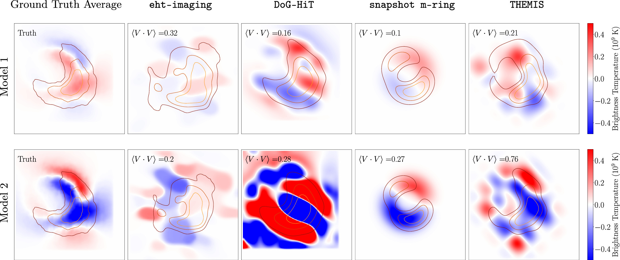
Figure 17. Circular polarimetric images of the two synthetic models across all methods, combining both days and bands. The posterior exploration results are means of the posterior distributions of images. The correlation coefficient 〈V · V〉 comparing to the associated ground truth is shown in the upper left corner of each reconstruction. The display scheme is analogous to that of Figure 11.
Download figure:
Standard image High-resolution imageWe present the linear polarization reconstructions of the two models in Figure 16. For each method we display the 2-day (April 6 and 7) and two-band (low and high) average results, indicating the normalized overlap in the linear polarization structure between the reconstructed image and the ground truth in the upper left corner. We quantify this overlap in terms of a correlation coefficient between the reconstructed and ground-truth linear polarization images, blurred to an effective resolution of 20 μas, as described in M87* Paper VII, where
The real part is chosen to measure the degree of alignment of the polarization vectors  . We present the circular polarization reconstructions of the two models in Figure 17, combining both days and bands. We also quantify a normalized overlap between the reconstructed and ground-truth circular polarization images, where
This metric is very sensitive to diffuse structure, which is more prominent in the circular polarization images, thus leading to worse overlap in circular polarization reconstruction across methods than linear polarization. The measured quantities presented in Figure 18 serve as an additional metric for reconstruction fidelity.
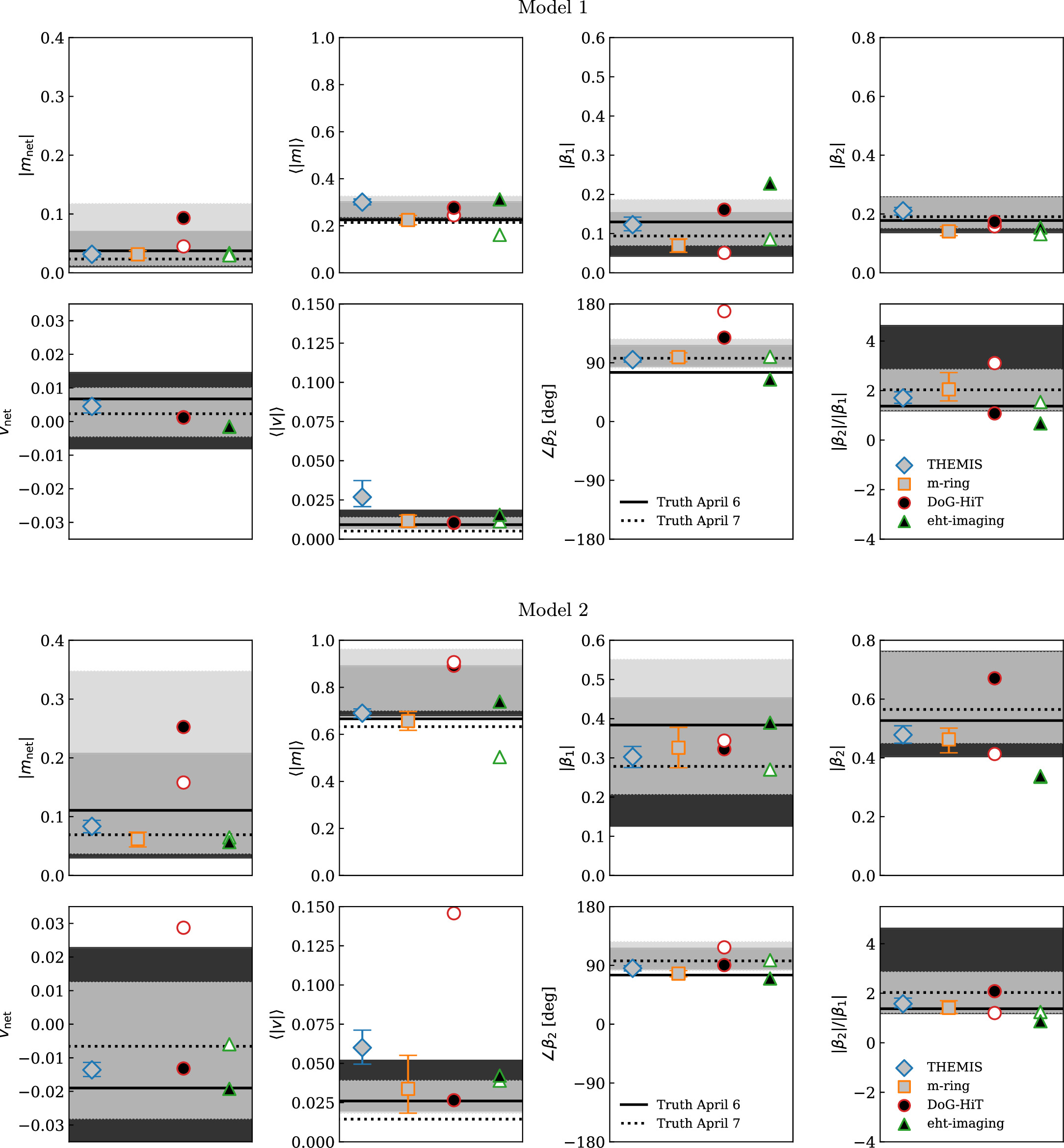
Figure 18. Comparisons of the measured linear and circular polarimetric quantities from the individual methods and the ground-truth average images of the GRMHD movies. The results for Model 1 are shown in the top eight panels, and the results for Model 2 are shown in the bottom eight panels. For the RML imaging methods, the filled and open symbols represent the April 6 and 7 results, respectively. The error bars for the snapshot m-ring and Themis methods represent the 90% confidence range from the day-combined posterior distributions. The ground-truth values are represented as filled and dashed lines for April 6 and 7, respectively. For DoG-HiT, which does not actively enforce  or
or  , we mask out any pixels that are below 10% of the peak intensity before calculating these quantities. The ground-truth GRMHD average images are blurred with a circular Gaussian 20 μas beam, as is done for the theory models compared to Sgr A* in Paper VIII. Horizontal lines represent the truth values for the average image, while shaded regions represent the 5th to 95th percentile regions spanned by individual snapshots for the two observing days. There is no measured m-ring value for vnet because the method fixes it to a value inferred from the ALMA light curve.
Download figure:
Standard image High-resolution imageWe note that for the snapshot m-ring modeling the mean image from posterior draws is constructed from the individual snapshot reconstructions, and so this mean image is not expected to fit the mean ground-truth image. Consistency is better shown via the measurable quantities from the entire posterior distribution. A comparison of the measurable polarimetric quantities to the ground truth is shown in Figure 18. Because 〈∣m∣〉 and 〈∣v∣〉 are resolution dependent, we apply a 20 μas Gaussian blurring kernel to the GRMHD simulations before computing truth values. All methods are generally able to recover the quantities of interest. The two posterior exploration methods, the snapshot m-ring modeling and Themis, perform comparably well, and better than the RML imaging methods. DoG-HiT has the most difficulty reconstructing the synthetic data as a consequence of its relatively weak assumptions on the distribution of the emission (it does not enforce  or
or  ). Based on the synthetic data performance and provided posterior distributions to quantify uncertainty, the m-ring and Themis Sgr A* results will be used for theoretical constraints, while the imaging results provide here a consistency check using inherently different methodologies.
Appendix C: Stokes Dependence

In this appendix, we describe a targeted test of the dependence of the polarimetric results on the underlying Stokes  structure. Paper III identified four clusters of total-intensity structure in the top-set images reconstructed for Sgr A*. Among these four clusters, three have a clear ring morphology with varying intensity patterns along the ring. Here we assume that Sgr A* has a ring morphology, and we test the choice of underlying ring mode in the polarimetric imaging.
In Figure 19, we show the reconstructed images for April 7 with both eht-imaging and DoG-HiT—the two softwares that make use of data that have been self-calibrated using the average total-intensity image—across the different total-intensity ring modes. In Table 7, we show the normalized overlap between the polarimetric structures of the ring modes and that of the average image used in the self-calibration for the primary results. While the total-intensity distribution along the ring differs, the polarization structure shows stability across ring modes. The main polarization properties are thus insensitive to the underlying total-intensity ring mode.
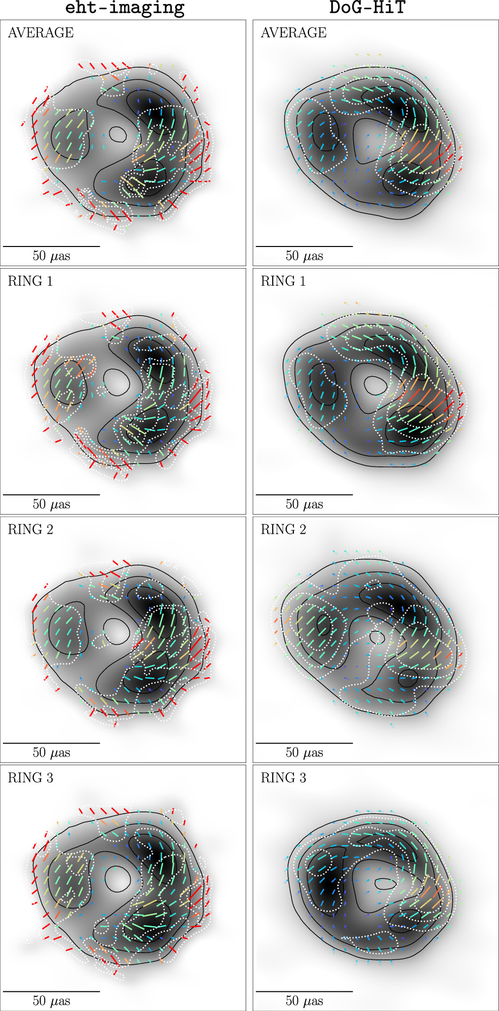
Figure 19. 2017 April 7 polarimetric images of Sgr A* with eht-imaging (left) and DoG-HiT (right), where the underlying Stokes  image (in gray scale) used in the self-calibration is chosen from the overall representative average image and the averages from the three ring clusters in Paper III. The display scheme is analogous to that of Figure 8.
Download figure:
Standard image High-resolution imageTable 7. The Normalized Correlation Coefficient between the April 7 Polarization Structure in the Ring Modes and That of the Average Image in Figure 19, for Both eht-imaging and DoG-HiT
| Ring Mode | eht-imaging | DoG-HiT |
|---|---|---|
| Ring 1 | 0.93 | 0.97 |
| Ring 2 | 0.88 | 0.85 |
| Ring 3 | 0.92 | 0.90 |
Download table as: ASCIITypeset image
Appendix D: Calibration Pipeline Dependence
While the main results in this work use the EHT-HOPS pipeline (Blackburn et al. 2019), we perform additional checks against the CASA rPICARD pipeline (Janssen et al. 2019) data. In Figure 20, we compare Sgr A* reconstructions from HOPS and CASA data for the 2017 April 6 and 7 observing days using identical analysis scripts with one RML imaging method (eht-imaging) and one posterior exploration method (snapshot m-ring modeling). We compute the polarization cross-correlation between the two reduction pipeline images, shown in the upper left corner of the CASA panels, and find good consistency. While the total-intensity images show some variation due to data differences, the same linear polarization structure for the CASA images is present on a large fraction of the ring, with a near-azimuthal EVPA pattern. In Figure 21, we compare the snapshot m-ring and eht-imaging reconstructions of the circular polarization in Sgr A* using HOPS and CASA data. For the snapshot m-ring method, the dipole structure along the ring, with a negative western region and a positive eastern region, is consistent for both pipelines. The eht-imaging reconstructions both prefer predominantly negative circular polarization, but the location differs owing to the variability in the data. Based on our confidence in each reconstruction method from the synthetic data tests, the main conclusions are generally robust to differences in calibration and reduction pathways.

Figure 20. Comparisons of reconstructions with eht-imaging and snapshot m-ring modeling using the HOPS (Blackburn et al. 2019) and CASA (Janssen et al. 2019) reduction pipelines combining days and bands. The HOPS images are those presented and used in the main body of this work. For each CASA image, the polarimetric cross-correlation is calculated against the equivalent HOPS image. The display scheme is analogous to that of Figure 8.
Download figure:
Standard image High-resolution image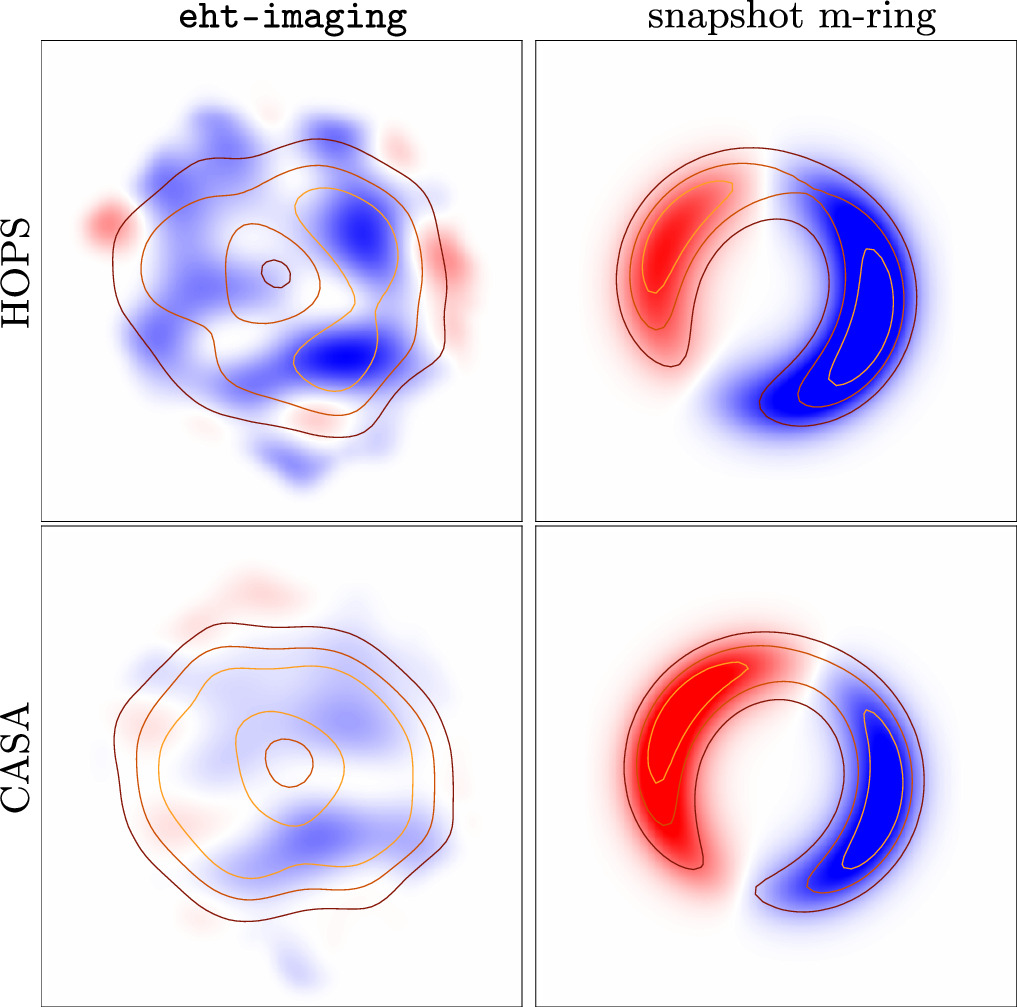
Figure 21. Comparisons of circular polarization reconstructions with eht-imaging and snapshot m-ring modeling using the HOPS (top) and CASA (bottom) reduction pipelines combining days and bands. The display scheme is analogous to that of Figure 11.
Download figure:
Standard image High-resolution imageFootnotes
- 155
- 156
- 157
While image structure may also induce variations in
, for sources smaller than 200 μas the visibilities are smoothed on 1 Gλ scales in the (u,v) plane. Thus, in the absence of an extended highly polarized component, variations on smaller (u,v) scales are evidence for temporal variability in the source. - 158
Note that this difference in variances does not imply that the fractional polarimetric variability is less than that of Stokes
, because the fractional polarimetric variability also depends on the degree of polarization.


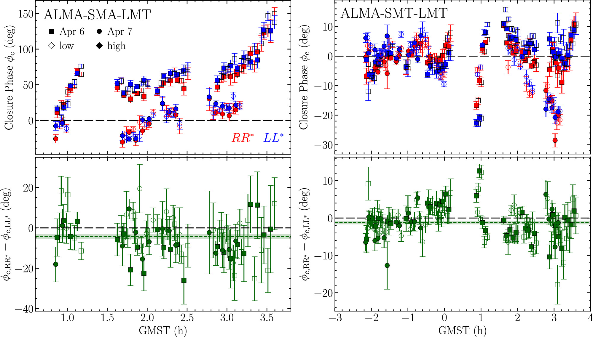