


Abstract
This paper examines the short- and mid-term periodicities (≲2 yr) in the cosmic-ray flux along 55 yr, from 1964 to 2019. The cosmic-ray flux has been computed by averaging the counting rates, in typified units, of a set of selected neutron monitors. This builds a representative virtual neutron monitor, named the global neutron monitor. The relevant discovered periodicities are ∼13.5, ∼27, ∼46–64, ∼79–83 day; Rieger-type (∼134–190 days); ∼225–309 day; and ∼1.06–1.15, ∼1.31–1.40, and ∼1.75–2.20 yr periods. The same analyses have been applied to the sunspot number (SSN) with the aim to compare the discovered periodicities and look for possible origins of these periodicities. Two main results have been achieved: the periodicities of 77–83 days, 134–190 days (Rieger type), 225–309 days, ∼1.3 yr, and ∼1.7 yr could be related to the solar dynamo, and an inversely linear relationship has been found between the average of the SSN versus the duration time for each solar cycle of the ∼1.75–2.20 yr period.
Export citation and abstract BibTeX RIS

Original content from this work may be used under the terms of the Creative Commons Attribution 4.0 licence. Any further distribution of this work must maintain attribution to the author(s) and the title of the work, journal citation and DOI.
| Glossary |
| • CRI: cosmic-ray intensity |
| • GNM: global neutron monitor |
| • GWS: global wavelet spectrum |
| • m.a.s.l: meters above sea level |
| • NH: northern hemisphere |
| • NMDB: neutron monitor database |
| • PCP: percentage of corrected points |
| • QBO: quasi-biennial oscillations |
| • SC: solar cycle |
| • SSN: sunspot number |
| • WPS: wavelet power spectrum |
Download table as: ASCIITypeset image
1. Introduction
Galactic cosmic rays are charged particles, mainly atomic nuclei, with energies between 106 and 1020 eV nucleon−1, originated in violent phenomena out of our solar system. The galactic cosmic-ray flux that reaches Earth at low energies (energies below several hundreds of GeV nucleon−1) is deeply affected by the solar cycle (SC) whose average time is 11 yr (Gnevyshev 1967). After entering the heliosphere, galactic cosmic rays are continuously modulated by the change in solar wind and the associated heliospheric magnetic field. Because of this, the cosmic-ray flux is at maximum during intervals of minimum solar activity and likewise their flux is at minimum during intervals of maximum solar activity (i.e., when the number of sunspots is at the maximum). Thus, cosmic-ray flux is anticorrelated to the solar activity, measured by the sunspot number (SSN), with perhaps some time delay caused by irregularities in the interplanetary magnetic field (Forbush 1958; Parker 1965; Usoskin et al. 1998; Singh et al. 2008; Chowdhury & Kudela 2018).
Usoskin et al. (1998) and Singh et al. (2008), among others, obtained that there is no lag between cosmic rays and SSN even during SCs. However, they verified that there is a time lag of 1 yr or more during the odd SCs. On the other hand, Chowdhury et al. (2016) reveal an abnormally long lag time between cosmic rays and SSNs of 10–17 months during SC24. Likewise, using Lomnický štít neutron monitor (NM) data, Chowdhury & Kudela (2018) obtained a long time delay of 15–18 months between NM counting rates and SSN during SC22 and part of SC24. Recently, Ross & Chaplin (2019), studying the long-term variations of cosmic-ray flux in relation to the SSN during SCs 20–24, found a time lag of 1–4 months between cosmic-ray flux in the even SCs (i.e., SC20, SC22, and SC24), and a time lag higher than 1 yr in the odd SCs.
The interaction with particles present in Earth's atmosphere also affects cosmic rays. Due to such interaction cascades of secondary particles (such as protons, muons, neutrons, and mesons) are created. Some of these secondary cosmic rays are detected by ground-based NMs and muon telescopes. In 1964, Hugh Carmichel developed an NM with a statistical accuracy of 0.1%, called NM64 (Shea & Smart 2000). Similar instruments along different locations on Earth have been developed subsequently. Most of them share their measurements in the Neutron Monitor Data Base 1 (NMDB) currently. To study solar activity it is necessary to use multiple stations located in different geomagnetic positions. The reason for this is that the position of NMs with respect to Earth's magnetic field determines the minimum energy for cosmic-ray particles to generate counts on a given station.
Nevertheless, a single NM representing a global behavior of the NM network can be useful for some studies. López-Comazzi & Blanco (2020) defined an NM representative of the NM network during the period of 2013–2018. This detector is named as the global neutron monitor (GNM).
The study of periodicities in NM counting rates has been a widely studied topic. There are many periodicity studies based on the power spectrum density obtained by the Fourier transform method, for example Attolini et al. (1975), among others. Other methods used for the detection of significant periodicities are the maximum entropy method (Valdés-Galicia et al. 1996) or the bispectral and Hilbert–Huang transform analysis (Vipindas et al. 2016). In recent times the most used analysis to carry out this detection of periodicities is the wavelet analysis as this method makes it possible to determine the evolution of periodicities over time, see for instance Kato et al. (2003), Adriani et al. (2018), Velasco Herrera et al. (2018), Singh & Badruddin (2019), or López-Comazzi & Blanco (2020). Other studies use several of these methods such as those in Kudela et al. (2010) and Tsichla et al. (2019). Some of the periodicities detected in NM counting rates that stand out from the mentioned studies are 27 day, quasi-biennial oscillations (QBOs) and an 11 yr period, and they are described below.
The cosmic-ray flux shows a periodic modulation of ≈27 days, associated with the solar synodic rotation and related to the coronal holes and corotating interaction regions (Grieder 2001). This period corresponds to the solar rotation at a latitude of 26° (Carrington rotation), consistent with the typical latitude of sunspots. The longitudinal asymmetry in the Sun is related to the 27 day period. This asymmetry is originated by both certain solar structures as large as the coronal holes and smaller irregularities potentially exhibiting a 27 day period (Poblet & Azpilicueta 2018). These researchers conclude that this period is not related to the solar electromagnetic radiation, therefore, reinforcing the role of structures, large and small, in the solar atmosphere. Additionally, solar active longitudes and tilted dipole structures have been associated with the 13.5-day period.
The Rieger-type period was observed for the first time in the gamma-ray flares around SC21 by Rieger et al. (1984) and by Kudela et al. (2002) in the cosmic-ray intensity throughout the interval of 1953–2000. This period is unstable and appears around solar maximum, coinciding with the change in polarity of the Sun. Gurgenashvili et al. (2016) performed a wavelet analysis of the SSN data from the Greenwich Royal Observatory and the Royal Observatory of Belgium during SCs 14–24 and they conclude that the Rieger-type periods occur in all of the SCs. The obtained Rieger-type period ranges from 155 to 200 days and they conclude that shorter Rieger-type periods occur during stronger SCs.
Under the name of QBOs are grouped periodicities with scales shorter than 11 yr, usually with timescales between ∼0.6 and 4 yr (Bazilevskaya et al. 2014a), although the most relevant QBOs change from ∼1.2 to ∼4 yr. These QBOs could probably reflect the intrinsic properties of the Sun related to the solar dynamo mechanism (Chowdhury et al. 2016, 2019). Among the QBOs, the 1.3 and 1.7 yr periods are specially relevant because they are probably periodicities related to the solar dynamo mechanism.
The 1.3 yr period, detected in the cosmic-ray flux, has been also reported in other solar and heliospheric features. Krivova & Solanki (2002) carried out a wavelet analysis of sunspot areas and SSNs detected this period. The 1.3 yr period shown in the solar rotation rate at the base of the convection zone can also be found in these solar activity data. They suggest that variations in the rotation rate do indeed have an influence on the workings of the solar dynamo. We must point out that this period coincides approximately with the eight subharmonics of the 11 yr period. This paper reveals a relationship between the 1.3 yr period and the Rieger period: specifically they consider that the Rieger period could be the third subharmonic of the 1.3 yr period. The 1.3 yr period has been also detected in variations of the interplanetary magnetic field and geomagnetic activity by Paularena et al. (1995). Based on the periodicity analysis in geomagnetic activity and solar wind, Mursula & Zieger (2000) conclude that the 1.3 yr period occurs during even SCs and the 1.7 yr period occurs during odd SCs. Valdés-Galicia et al. (1996) and Velasco Herrera et al. (2018) have reported a period of 1.7 yr in the NM counting rates. According to these papers, this period is related to emergence and transportation phenomena of the magnetic flux and is a multiple of the Rieger period. Concretely, the 1.7 yr period is correlated with fluctuations of similar periodicity found in large active regions and the equatorial southern coronal area. These regions are zones in the Sun where the magnetic flux is generated. Finally, Tsichla et al. (2019) detected this periodicity in the geomagnetic index Ap and cosmic-ray flux in the time interval of 1965–2018 using a wavelet analysis and fast Fourier transform (FFT).
The 11 yr period, which is the most prominent periodicity recorded in NM counting rates, is related to the inversion of the solar global magnetic field. The number of all the structures in the solar atmosphere, for instance sunspots, filaments, coronal holes, or the number of transitory events as flares or coronal mass ejections, changes along with the solar magnetic field variation. This was already covered in Gnevyshev (1967). Cosmic-ray flux anticorrelates with the number of structures/events commented above reflecting also its dependence with the SC and so with the variation of their propagation conditions linked with the solar magnetic field.
Rossby waves have been proposed by recent studies to explain some of the periodicities observed in solar activity. The instabilities on the solar magnetic field caused by solar Rossby waves in the Sun's interior might indirectly be affecting the activity of the heliosphere and Earth's atmosphere (Silva & Lopes 2017). Therefore, this variation can also affect the NM counting rates. Specifically, the QBOs detected in the NM counting rates could be an indirect consequence of the Rossby magnetic waves.
Being a self-sustaining dynamo, the Sun transforms convective motion and differential rotation to electromagnetic energy. Therefore, the solar magnetic field is produced by the solar dynamo. The detailed mechanism of the solar dynamo is unknown and is currently under study (Tobias 2002; Dikpati et al. 2017). Current models place the solar dynamo in the tachocline. The tachocline is a transition zone between the convective region and the radiative zone and is located at a distance of ∼0.7 R⊙ with an average thickness of ∼0.04 R⊙, where R⊙ is the solar radio (Hughes et al. 2007). The radiation zone rotates as a rigid solid while the convection region shows differential rotation. This fact causes a shearing effect on the tachocline. Gilman (2000) points out that the magnetic field must be toroidal, with no poloidal component. The magnetohydrodynamic "Shallow Water" model predicts the presence of waves in the tachocline. Dikpati et al. (2017) suggest that if these waves are generated in the tachocline, their effect may manifest on the solar surface. Rossby waves are a consequence of the conservation law of angular momentum and their velocity is proportional to the rotational velocity of the system. The solar magnetic field exerts a strong influence on these waves causing two modes to appear: one traveling westward, very similar in its characteristics to the hydrodynamic case (fast Rossby magnetic waves), and another slower mode that travels eastward with longer periods of time (slow Rossby magnetic waves; Zaqarashvili et al. 2007).
Since slow Rossby magnetic waves have very long periods in the order of centuries and thousands of years, we focused only on fast Rossby waves. Fast Rossby magnetic waves have the characteristic that in the presence of a moderate magnetic field they become equatorially confined as the rotational speed of the system increases.
For this work, we establish the following operative classification: short-term periodicities refer to periods from 2 days to about 30 days, mid-term periodicities are those periods found in the range between 30 days and 2 yr, and long-term periodicities refer to periods greater than 2 yr. This paper examines the short- and mid-term periodicities during the period 1964–2019 in GNM using the wavelet technique (Torrence & Compo 1998). GNM is a virtual station whose counting rates have been obtained by averaging the counting rates, in typified units, of all selected NMs for a particular SC.
The main objective of this work is to study the periodicities in the cosmic-ray counting rate along the longest ever studied period (from 1964 to 2019) using a single NM, the GNM, which is representative of the NM network in this kind of study. We determined the periodicities in the GNM and SSN throughout the interval described above and the values of the cross-correlation function between GNM and SSN. Finally, we explore whether there is a relationship between fast Rossby magnetic waves and the short- and mid-term periodicities obtained in the solar activity and GNM counting rates.
2. Data and Analysis Methods
2.1. Global Neutron Monitor
Different NM sets have been selected to build the GNM for each SC. Table 1 lists the names of the stations used in this work along with their latitude, longitude, height (in meters) above sea level (m.a.s.l.), vertical cutoff rigidity, and a coefficient that indicates whether the station is in the northern hemisphere (NH = 1) or the southern hemisphere (NH = 0). The data are 1 hr pressure-corrected counting rates and were collected from the NMDB web page 2 and the Network of Cosmic ray Stations. 3 We consider five time intervals: SC20 (from 1964 October 1 to 1976 February 29), SC21 (from 1976 March 1 to 1986 August 31), SC22 (from 1986 September 1 to 1996 July 31), SC23 (from 1996 August 1 to 2008 November 30), and SC24 (from 2008 December 1 to 2019 January 31). A check of the data availability in these webs was performed initially. For each considered interval, only stations with less than 5% of the missing values and outliers were selected to make up the GNM.
Table 1. Features of the Different Selected Neutron Monitors Used in This Work
| ID | Station | Latitude (deg) | Longitude (deg) | Rc (GV) | Altitude (m.a.s.l.) | NH |
|---|---|---|---|---|---|---|
| AATA | Alma-Ata | 43.14 | 76.60 | 6.69 | 3340 | 1 |
| APTY | Apatity | 67.57 | 33.39 | 0.65 | 181 | 1 |
| CALG | Calgary | 51.08 | −114.13 | 1.08 | 1128 | 1 |
| CLMX | Climax | 39.37 | 106.18 | 2.99 | 3400 | 1 |
| DRBS | Dourbes | 50.10 | 4.60 | 3.18 | 225 | 1 |
| FSMT | Fort Smith | 60.02 | −111.93 | 0.30 | 180 | 1 |
| HRMS | Hermanus | −34.43 | 19.23 | 4.44 | 26 | 0 |
| INVK | Inuvik | 68.36 | −133.72 | 0.30 | 21 | 1 |
| IRKT | Irkutsk | 52.47 | 104.03 | 3.64 | 475 | 1 |
| JUNG | Jungfraujoch (IGY) | 46.55 | 7.99 | 4.49 | 3570 | 1 |
| JUNG1 | Jungfraujoch (NM64) | 46.55 | 7.99 | 4.49 | 3475 | 1 |
| KERG | Kerguelen | −49.35 | 70.25 | 1.14 | 33 | 0 |
| KIEL | Kiel | 54.34 | 10.12 | 2.36 | 54 | 1 |
| LMKS | Lomnický štít | 49.2 | 20.22 | 3.84 | 2634 | 1 |
| MCMU | Mc Murdo | −77.90 | 166.60 | 0.30 | 48 | 0 |
| MGDN | Magadan | 60.04 | 151.05 | 2.10 | 220 | 1 |
| MOSC | Moscow | 55.47 | 37.32 | 2.43 | 200 | 1 |
| MRNY | Mirny | −66.55 | 93.02 | 0.03 | 30 | 0 |
| NAIN | Nain | 56.55 | −61.68 | 0.30 | 46 | 1 |
| NEWK | Newark | 39.68 | −75.75 | 2.40 | 50 | 1 |
| NVBK | Novosibirsk | 54.48 | 83.00 | 2.91 | 163 | 1 |
| OULU | Oulu | 65.05 | 25.47 | 0.80 | 15 | 1 |
| PSNM | Princess Sirindhorn | 15.59 | 98.49 | 16.80 | 2565 | 1 |
| PTFM | Potchefstroom | −26.68 | 27.10 | 6.94 | 1351 | 0 |
| ROME | Rome | 41.86 | 12.47 | 6.27 | 0 | 1 |
| SNAE | Sanae | −71.67 | −2.85 | 0.73 | 856 | 0 |
| SOPO | South Pole | −90.00 | 0.00 | 0.10 | 2820 | 0 |
| TERA | Terre Adelie | −66.65 | 140.02 | 0.01 | 32 | 0 |
| THUL | Thule | 76.50 | −68.70 | 0.30 | 26 | 1 |
| YKTK | Yakutsk | 62.01 | 129.43 | 1.65 | 105 | 1 |
Note. From left to right: identifier of the station into the NMDB, station name, latitude, longitude, current vertical cutoff rigidity, height above sea level (in meters), and the NH coefficient . The NH coefficient has a value equal to 1 if the station is located in the northern hemisphere and 0 if it is located in the southern hemisphere.
Download table as: ASCIITypeset image
An atypical value or outlier is an observation that is numerically distant from the rest of the data. These outliers must be removed or replaced by other values. To carry out outlier detection we apply the analysis of box and whiskers, which depends only on the data itself and not on the distribution of the data. This analysis was applied separately for each NM in each SC. The points out of the range ![$\left[{Q}_{1}-1.5\left({Q}_{3}-{Q}_{1}\right),{Q}_{3}+1.5\left({Q}_{3}-{Q}_{1}\right)\right]$](https://content.cld.iop.org/journals/0004-637X/927/2/155/revision3/apjac4e19ieqn1.gif) , being Q1 and Q3 the first and third quartile, respectively, were considered outliers. The set of outliers and missing values were substituted by linear interpolation. The percentage of bad points (missing values and outliers) with respect to the total set of data for a given NM in each SC is collected, together with the final selection of stations in each SC, in the table located in the Appendix in the percentage of corrected points (PCP) column. The stations with a PCP >5% were left out of the analysis for reasons explained above. It is important to highlight that the Forbush decreases and that ground-level enhancements are detected in the GNM counting rate. None of them are affected by the outlier criterion taken in this work.
, being Q1 and Q3 the first and third quartile, respectively, were considered outliers. The set of outliers and missing values were substituted by linear interpolation. The percentage of bad points (missing values and outliers) with respect to the total set of data for a given NM in each SC is collected, together with the final selection of stations in each SC, in the table located in the Appendix in the percentage of corrected points (PCP) column. The stations with a PCP >5% were left out of the analysis for reasons explained above. It is important to highlight that the Forbush decreases and that ground-level enhancements are detected in the GNM counting rate. None of them are affected by the outlier criterion taken in this work.
The graphical representation of the data allows for the detection of patterns or anomalies that can hardly be detected by numerical statistical analysis. In this way, we depict counting rates of the selected NMs in each SC with the objective of detecting anomalous behaviors. Counting rates showing sudden jumps that are maintained over time were not taken into account in the selection. Finally, 13, 18, 22, 17, and 12 NMs were selected for the SC20, SC21, SC22, SC23, and SC24, respectively. Only four stations, the Apatity NM (APTY), the Moscow NM (MOSC), the Newark NM (NEWK), and the Oulu NM (OULU), verified the selection condition (PCP < 5%) for all of the considered SCs.
To confirm that the selected stations show a similar behavior, which allows one to compare them and therefore be used to build the GNM, we make use of three quality indices defined in López-Comazzi & Blanco (2020). These quality indices are referenced as Qj , Qx , and Qu which, by distinct methods, compare the different NMs in each SC and give us a quantitative idea of which stations have a distant behavior of the general trend.
Only those NMs with Qj , Qx , and Qu > 0.5 are included in the determination of the GNM. We decided to use a threshold of 0.5 because statistical studies consider a value equal or greater than ±0.5 of the cross-correlation function as a moderate linear association that is positive or negative, depending of the sign. Considering that the coefficients Qx and Qu also use the cross-correlation function, the same criterion was taken into account. We also apply this criterion to the coefficient Qj . It is considered that Qj > 0.5 indicates that the difference between two spectra is marginal.
The Qj index evaluates how much a single power spectrum of a certain station in a determined SC differs from the one that is obtained by the average of all stations in that SC. Qx is the weighted cross-correlation between a single NM counting rate in a certain SC and the other stations in that SC. Qu is determined following the same procedure used to calculate Qx , but it is applied to the power spectrum and not to the counting rates.
Table 6 in the Appendix shows the Qj , Qx , and Qu , PCP, and the delay h of the selected NMs, along SCs 20–24, ordered according to the quality index Qj . The values of Qj , Qx , and Qu for these stations are also shown and in all cases we see that they exceed the value of 0.5. The values of PCP by linear interpolation, and h, the delay of each station with respect to OULU, are also collected.
The counting rate at a given station is a function of cutoff rigidity, altitude, and the building where the NM is located, among other factors. However, we propose a virtual NM whose counting rates can be representative of the response on the NM counting rates to solar activity.
We define GNM as a virtual NM whose counting rate is obtained using the average of all the counting rates, in typified units or reduced centered units, of all the selected NMs in a particular study. The construction of the GNM is carried out for every SC separately.
Although the complete procedure to build the GNM is extensively described in López-Comazzi & Blanco (2020), a brief summary is written below. The typified unit of the counting rates in a discretized time n is given by

where xn
is the counting rate in a discretized time n in any NM, and  and σx
are the mean and standard deviation, respectively. This reduced centered variable has a null mean (
and σx
are the mean and standard deviation, respectively. This reduced centered variable has a null mean ( = 0) and a standard deviation equal to 1 (σz
= 1).
= 0) and a standard deviation equal to 1 (σz
= 1).
Once zn is computed for an NM, we calculate the delay or temporary advance h between a single NM and an OULU NM in each SC. OULU is taken as the reference station and the delays of the other stations with respect to OULU are calculated. The selection of OULU as the reference station was made arbitrarily among the four stations present in all of the SCs. The delay h for a given station x in each SC is the value between −100,.., −1, 0, + 1,.., +100 (hours), which maximizes the normalized cross-correlation function ρxy in each SC.
This function is given by
where x is a single NM counting rate, y is OULU NM counting rate, and
is the sample cross-correlation or cross-covariance, N is the number of points in that SC, xn+h
is the counting rate of a particular NM in a discretized time n + h, yn
is the counting rate of OULU NM in a discretized time n to be compared with the first one, and  and
and  are the average values of each time series, respectively.
It is accepted that a cross-correlation coefficient ρxy is statistical significant, at a 95% confidence interval, if
where N − h is the number of data points used in the calculation of the ρxy
for each SC being that h = 0, ± 1,.., ± 100 the lag. In this case, ρxy
is statistically significant for the obtained values in this work. Finally, the cross-correlation function between OULU NM and the rest of the stations in each SC is computed, keeping the maximum value of  .
.
Once the delays of the selected NMs are computed, the time for each NM is shifted according to the respective obtained delays. This puts the selected NM at the OULU time.
Figure 1 (upper panel) displays the GNM counting rate from 1964 October 1 to 2019 January 31. Every SC is plotted in different colors to make analysis easier. The polarity reversal intervals (vertical black lines) have been selected according to Lantos (2005). The sign of the polarity of the solar magnetic field changes every ∼11 yr. When the direction of the solar magnetic field is outward from the Sun in the north polar region, the polarity is positive (A > 0). In this case, particles with a positive charge drift inward in the poles of the heliosphere and outward along the heliospheric current sheet. On the contrary, when the solar magnetic field points in the opposite direction (i.e., inward from the Sun), the polarity is negative (A < 0). Depending on the sign of the polarity, the cosmic-ray intensity maxima have a different shape (Bazilevskaya et al. 2014b; Chowdhury & Kudela 2018).
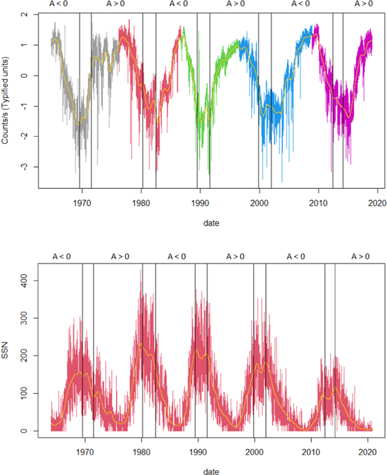
Figure 1. Upper panel: GNM counting rates (in typified units) in each SC. The GNM counting rates in SC20 are represented in gray, in red SC21, in green SC22, in blue SC23, and in pink SC24. Lower panel: SSN as a function of time. The yellow line was obtained by a smoothing function using a local polynomial regression (loess) with α = 0.025 in both cases.
Download figure:
Standard image High-resolution imageAlternating polarity states of the Sun are indicated at the top of the figure. One can see that when the polarity is positive (A > 0) the curve of the GNM counting rates shows a flat-topped shape, while when the polarity is negative a peaked shape is shown (A < 0). The alternating peaked and flat-topped shapes of the GNM counting rates in Figure 1 (upper panel) are the manifestation of the alternating polarity of the solar magnetic field in addition to other cosmic-ray transport processes (Aslam & Badruddin 2012).
2.2. Sunspot Number
Sunspots are darker areas on the solar photosphere because their temperature is ∼1500 K lower than the closest environment. They are also characterized by intense magnetic fields. The sunspots are not randomly distributed on the solar disk. When the cycle of activity begins, they appear at high latitudes, then their emerging point begins to descend to be located at the maximum between 30° and 10° latitude, and at the end of the cycle, in the vicinity of the solar equator. Some of them are up to 5 × 10⁴ km wide. Sunspot lifetime ranges from hours to weeks. This implies that the spatial distribution of sunspots may vary with each solar rotation. The SSN is calculated as

where Ns is the number of individual spots, Ng is the number of sunspot groups, and K is the scaling coefficient, usually less than unity. The relative SSN is an index of the activity of the entire visible disk of the Sun. It is determined each day without reference to the preceding days. Figure 1 (lower panel) shows the SSN as a function of time along the studied interval. The anticorrelation between solar activity and the GNM counting rates is shown in Figure 1.
To establish a comparison of NM behavior and solar conditions, we have taken daily observations of international SSN from https://www.ngdc.noaa.gov/stp/SOLAR/ as complementary data.
2.3. Time-lag Analysis between Global Neutron Monitor Counting Rates and Sunspot Numbers
The observed periodicities in the GNM counting rates and SSN show their maximum power spectra at different moments along the SC and these moments are not the same for some of the characteristic periods for cosmic rays or SSNs. One reason for this could be a result of a shift between the time when cosmic ray/SSN reach minimum/maximum at the solar maximum. To bring some light to this, a similar approach to that developed by Usoskin et al. (1998) and Ross & Chaplin (2019) to investigate the time delay between the modulation of the cosmic-ray intensity compared to the solar activity has been followed. A time-lag cross-correlation analysis was performed between daily averaged GNM counting rates and daily averaged SSN. For this purpose, daily averages have been calculated from the hourly GNM data.
We used a temporal window with a width of T = 1200 days centered at time t, shifting within the interval [t − T/2, t + T/2]. The window was shifted in steps Δt = 1 day and for each step the normalized cross-correlation coefficient ρ, given by Equation (1), between the GNM counting rates and the SSN was computed.
The delay h between the GNM counting rates and the SSN in each SC is the value that minimizes the normalized cross-correlation function in each SC. Ross & Chaplin (2019) used the Spearman's rank correlation coefficient instead of the normalized cross-correlation coefficient but in our case the former is not used because it can only be applied to small data samples.
A time-lag cross-correlation analysis between the GNM counting rates and the SSN was conducted to determine if there is a certain delay that may explain why some periodicities are detected in the GNM and not in the SSN or why they show a different time.
The cross-correlation function ρ between the GNM and the SSN is shown in Figure 2. The y-axis order has been inverted. One can observe that this variation in ρ presents an anticorrelation with the solar activity as expected. Clear, different behaviors are observed for the odd and even cycles: a maximum anticorrelation with a lag of 4–6 days in present the even SCs while the lag is 100–300 days in the odd SCs (see Table 2).
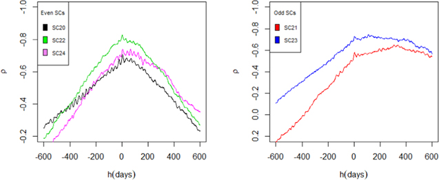
Figure 2. Variation in the normalized cross-correlation function with time lag h between the GNM counting rates and the SSN in the even SCs (left panel) and the odd SCs (right panel).
Download figure:
Standard image High-resolution imageTable 2. Time Lags h and the Corresponding Normalized Cross-correlation Coefficient ρ between the GNM Counting Rates and the SSN for SCs 20–24
| Solar Cycle | h (days) | ρ | |
|---|---|---|---|
| Even | 20 | 6 | −0.707 |
| Odd | 21 | 307 | −0.645 |
| Even | 22 | 4 | −0.826 |
| Odd | 23 | 111 | −0.744 |
| Even | 24 | 6 | −0.737 |
Download table as: ASCIITypeset image
Several studies, such as Usoskin et al. (1998), Singh et al. (2008), and Ross & Chaplin (2019), have demonstrated that the lag between the cosmic-ray counting rates and solar activity is approximately zero during the even SCs and a lag exists around 1 yr during the odd SCs. These results are in agreement with our study, although in the SC23 we obtained a lag of 111 days, which is one-third of the delay obtained in these works. Therefore, a clear, different behavior exists between the odd and even SCs, and this could be reflected in the frequencies observed in NM counting rates. This will be discussed in the following section as a reference of NM behavior using the GNM defined in Section 2.1.
2.4. Wavelet Analysis
Wavelet analysis is a tool for analyzing localized variations of spectral power within a time series. This analysis decomposes a time series into a sum of wavelets that come from a "mother" wavelet function (the Morlet function). The continuous, normalized wavelet transform applied to a discrete sequence xn with equal temporary spacing δ t and time index n = 0, ..., N − 1 is
where xn are the different points of the time series at time index n, Ψ* is the conjugate complex of the "mother" wavelet function, and the coefficients s are relative to the scale of the wavelet.
Concretely, we used the "mother" Morlet function, given by

where ω0 = 6 is the dimensionless frequency and η = s · t. Spectral power P is computed following P = ∣Wn (s)∣2. The wavelet power spectrum (WPS) refers to the temporal evolution of P with each frequency. Another perspective is given by the global wavelet spectrum (GWS), which is the spectral power averaged at each frequency s:

The WPS of the GNM counting rates and SSN are collected in Figures 5 and 6, respectively. The GWS of the GNM counting rates and SSN are collected in Figures 3 and 4.

Figure 3. GWS of the GNM in each SC. d denotes days and y denotes years. The red line shows the 95% confidence level. The peaks above this line are considered significant periodicities.
Download figure:
Standard image High-resolution image
Figure 4. GWS of the SSN in each SC. d denotes days and y denotes years. The red line shows the 95% confidence level. The peaks above this line are considered significant periodicities.
Download figure:
Standard image High-resolution imageThe WPS is given by a heat map, where lower values of the spectral power are depicted by the color blue, intermediate values are in green and yellow, and the higher values of spectral power are shown in red. The GWS is a curve that shows the average spectral power, throughout the entire interval, associated to each period.
In this work, a frequency is considered significant when it shows a confidence level above 95% in the GWS. The black line in the WPS figures (Figures 5 and 6) represents frequencies verifying this criterion. The shaded area in WPS figures shows the cone of influence, corresponding to the zone influenced by the edge effects.
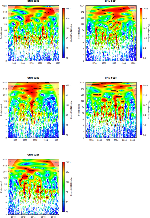
Figure 5. Wavelet power spectrum of GNM in each SC.
Download figure:
Standard image High-resolution image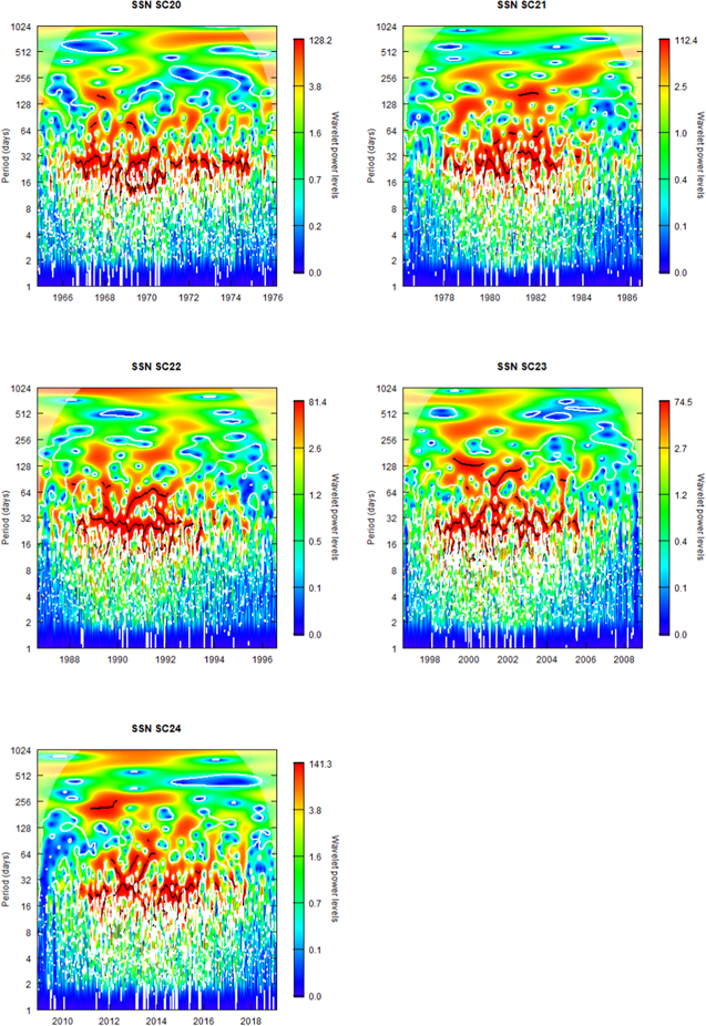
Figure 6. Wavelet power spectrum of SSN in each SC.
Download figure:
Standard image High-resolution image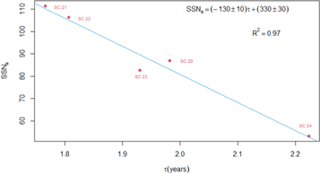
Figure 7. Mean of the SSNa in each SC vs. time of T ∼ 1.7 yr period (τ) in years obtained in the GNM counting rates.
Download figure:
Standard image High-resolution imageThe significance level above which P = ∣Wn (s)∣2 represents a real characteristic of the time series is obtained by comparison with a reference background signal. This reference signal can be modeled as white noise or red noise. A simple model for the red noise is the univariate lag-1 autoregressive process (Torrence & Compo 1998). The Fourier spectrum of this model is given by
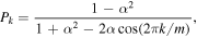
where k = 0, .. ,m/2 is the frequency index and
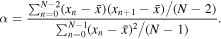
xn
is a time series in the discretized time n, and N and  are the number of points and the average value of these time series, respectively.
We determine the 95% confidence level (significant at 5%), multiplying the background spectrum Pk by the 95th percentile value for chi-squared distribution χ2 function with two degrees of freedom. The periodicities collected in Tables 3 and 4 are in the 95% confidence level. The R package "WaveletComp" developed by Angi Röesch and Harald Schmidbauer has been used to perform the wavelet analysis of time series (see Roesch & Schmidbauer 2018).
Table 3. Short-term and Mid-term Periodicities Detected in the GNM Counting Rates in Each Solar Cycle and throughout the Entire Interval
| GNM Counting Rates | |||||||||
|---|---|---|---|---|---|---|---|---|---|
| SC20 | 13.5 d | 27 d | ⋯ | 83 d | 190 d | ⋯ | 1.06 y | 1.40 y | 1.98 y |
| SC21 | 13.5 d | 27 d | ⋯ | 79 d | 153 d | 302 d | ⋯ | ⋯ | 1.77 y |
| SC22 | 13.5 d | 27 d | ⋯ | 81 d | 213 d* | ⋯ | ⋯ | 1.31 y | 1.81 y |
| SC23 | 13.5 d | 27 d | 64 d | ⋯ | 134 d | 225 d | 1.11 y | ⋯ | 1.93 y |
| SC24 | 13.5 d | 27 d | 46 d | ⋯ | 140 d | 309 d | ⋯ | 1.37 y | 2.20 y |
| SCs 20–24 | 13.5 d | 27 d | ⋯ | 76 d | 151 d | 308 d | 1.15 y | ⋯ | 1.75 y |
Note. d denotes days, y denotes years, and * refers to a period that does not meet the percentage criterion given by Equation (6), but has been grouped in the Rieger period column for other reasons that are explained in the text.
Download table as: ASCIITypeset image
Table 4. Short- and Mid-term Periodicities Detected in the SSN in Each Solar Cycle and throughout the Entire Interval
| SSN | ||||||||||
|---|---|---|---|---|---|---|---|---|---|---|
| SC20 | 13.5 d | 27 d | ⋯ | 77 d | ⋯ | 141 d | ⋯ | 0.99 y | ⋯ | 2.06 y |
| SC21 | 13.5 d | 27 d | 53 d | ⋯ | 124 d | 160 d | 301 d | ⋯ | 1.26 y | ⋯ |
| SC22 | 13.5 d | 27 d | 57 d | ⋯ | ⋯ | 161 d | ⋯ | 1.07 y | ⋯ | 1.86 y |
| SC23 | 13.5 d | 27 d | ⋯ | ⋯ | 124 d | ⋯ | ⋯ | 0.99 y | ⋯ | 2.08 y |
| SC24 | ⋯ | 27 d | 46 d | ⋯ | 106 d | ⋯ | 239 d | ⋯ | ⋯ | 1.89 y |
| SCs 20–24 | 13.5 d | 27 d | ⋯ | ⋯ | ⋯ | 149 d | 312 d | ⋯ | ⋯ | ⋯ |
Note. d denotes days and y denotes years.
Download table as: ASCIITypeset image
3. Results and Discussion
The GNM defined above has been built with the goal to obtain a single representative measurement of global NM network along 55 yr. A wavelet analysis was applied to determine such periodicities. Possible periodicities have been found in an interval ranging from 2 to 1024 days for the GNM and SSN throughout the whole interval (1964–2019).
Changes in cosmic-ray propagation conditions in the heliosphere produce variations in the flux of cosmic rays observed by ground-based NMs, resulting both in periodicities maintained in time and nonperiodic variation caused by solar activity transients. Moreover, there are other circumstances that can affect the expected NM counting rate such as magnetic cutoff rigidity, altitude, or the building where the monitor is located, among others. We propose a virtual monitor (GNM) whose counting rate can be representative of the variation of counting rates to changes in the cosmic-ray propagation conditions or solar activity. The SSN is a parameter, among others such as solar wind speed or heliospheric magnetic field, that should reflect possible changes on the propagation conditions of cosmic rays in the heliosphere and monitor the solar cycle status. For this reason, the SSN has been chosen as a proxy of solar activity and so, as a proxy of global cosmic-ray propagation conditions to be compared to the cosmic-ray counting rate and to analyze the discovered periodicities.
The detected periodicities in the GNM counting rates are 13.5 and 27 day periods, a period around 46–64 days, a period around 79–83 days, a 134–190 day period (Rieger-type period), 225–309 day period, ∼1 yr period, ∼1.3 yr period, and ∼1.7 yr period and they are listed in Table 3. The periodicities detected in the GNM counting rates in each SC are identified by the significant peaks obtained in Figure 3 following the significance level criterion described in Section 2.4.
The same procedure has been applied to SSNs where the significant periodicities are marked by the period duration shown in Figure 4. The periodicities detected in the SSN are 13.5 and 27 day periods, a period around 46–64 days, 77 day period, a period around 106–124 days, 141–161 day period (Rieger-type period), a period around 239–301 days, ∼1 yr period, ∼1.3 yr period, and ∼1.7 yr period and they are collected in Table 4. All periods detected in the SSN appear in the GNM with the exception of the period around 106–124 days.
Denoting Ti
the set of periodicities grouped in a column, being  ,
,  as the maximum and minimum times of the periodicities of column i and mean(Ti
) the average of the periodicities grouped in that column, we use the equation
as the maximum and minimum times of the periodicities of column i and mean(Ti
) the average of the periodicities grouped in that column, we use the equation

to establish a criterion to determine whether they are the same periodicity. For example, in the last column  ,
,  and mean(T∼1.75y
) = 1.94y. These values yield a percentage of 22%, therefore, we consider that the set
and mean(T∼1.75y
) = 1.94y. These values yield a percentage of 22%, therefore, we consider that the set  has a common origin. We consider that the periodicities selected in each column correspond to a common origin if perc is less than 35%. The periodicities in Tables 3 and 4 have been grouped in columns according to this criterion.
We complete the analysis with the WPS that allow us to determine in which intervals of the SC the detected periodicities appear. The WPS of the GNM counting rates and the SSN for SCs 20–24 are displayed separately in Figures 5 and 6, respectively. Periods up to 1024 days, i.e., the maximum duration to include the short-term and mid-term periodicities as defined in the 1, are shown in these figures. As a general comment, the periodicities in Tables 3 and 4 used to be more clearly identified around the solar maximum and less marked in the solar minimum.
The GNM counting rates show a strong periodicity of 27 days, related to solar synodic rotation, in all SCs. Concretely, the 27 day periodicity is the second strongest peak below that of the 1.7 yr period (Figure 3) in all SCs. This period also appears in the SSN, which in this case is the most prominent among all the observed periodicities (Figure 4). The period of 13.5 days also appears in both spectra, i.e., GNM and SSN, but with less intensity. We must to point out that for the SSN this period is hidden by a stronger 27 day period in SC23 and SC24. The 13.5 and 27 day periods appear throughout the complete time series except at solar minima. On the other hand, although SC22 presents the same persistence of both periodicities, they both show a lower spectral power (Figure 5). The 13.5 and 27 day periods in the SSN are also persistent throughout all SC maxima disappearing in solar minima in coincidence with the sunspot disappearance (Figure 6).
A periodicity between 79 and 83 days appears in the GWS of the GNM in SCs 20, 21, and 22. In the SSN this period only appears in SC20. This period could be due to a Rossby wave, which will be discussed in detail below. A period between 46 and 64 days is detected in SCs 23 and 24 in the GNM. The GWS of the SSN shows a period between 46 and 53 days in SCs 21, 22, and 24. The 46–64 day period could correspond to the second harmonic of the solar rotation. Periodicities of 63 and 84 days were reported in the SSN during SC23 by Joshi et al. (2006).
The period between 106 and 124 days is clearly observed in the SSN in SCs 21, 23, and 24. However, this period is not observed in the GNM. This circumstance may lead to the conclusion that the process that may be behind this periodicity does not have an influence on the conditions of cosmic-ray propagation through the heliosphere. The hidden process that gives rise to the occurrence of this period is something that we should study in the future. This periodicity of 106–124 days has already been reported by Joshi et al. (2006) in the SSN.
Zones of high spectral power are observed between 32 and 128 days, where the periodicities of 46–64 days and 79–83 days are found in certain parts of the ascending and decreasing phases of the SC20 and SC21 in WPS of the GNM. However these zones are observed around the solar maximum in SCs 22–24, disappearing in the rest of the cycle. This last observation is especially evident in SC22. The WPS of the SSN in this 32–128 day range shows a similar behavior to the WPS of the GNM with high spectral power values, in red, around the solar maxima in all SCs. The spectral power has high values in this range of solar maxima in the WPS of the SSN, so that the possible real periodicities are superimposed, making it difficult to differentiate them and determine their evolution.
Rieger-type periods (134–190 days) have been found in the GNM in all SCs except for SC22. This periodicity is detected with high spectral power exclusively in the Sun's magnetic polarity reversal intervals in these four SCs in the GNM. Then, the Rieger-type period could be related to the solar dynamo mechanism. The 213 day period is considered to be a Rieger period even though the value of the period, 213 days, is far from the typical value of the Rieger period of 151 days. The reason for this decision is that this period occurs during solar maximum as is the case for the Rieger period in the rest of the solar cycles considered and is the closest to the expected Rieger period. This period has been marked with an asterisk in Table 3. The Rieger-type period was detected in the SSNs in SCs 20, 21, and 22. Nevertheless, Gurgenashvili et al. (2016) detected the Rieger-type period in all cycles spanning SCs 14–24. Concretely, they obtained a period between 155 and 197 days in each cycle from SCs 20–24.
A periodicity slightly below a year, 225–309 days, appears in the GNM in SCs 21, 23, and 24. This period is also detected in the SSN in SCs 21 and 24. A period longer than 1 yr appears in the GNM in SCs 20 and 23 and in the SSN in SCs 20, 22, and 23.
The 1.3 yr period has been found in the even SCs, i.e., SCs 20, 22, and 24 in GNM. In contrast, in the SSN, a 1.3 yr period is only clearly observed in SC21. Krivova & Solanki (2002) detected this period in the SSN by analyzing data from 1874 to 1997.
The 1.3 yr period seems to disappear during SCs with negative polarity, A < 0, when the cosmic-ray maximum is strongly peaked and incoming cosmic-ray drift is along the solar magnetic equator, appearing during A > 0 cycles when the cosmic-ray maximum shows a long plateau and cosmic-ray incoming drift happens throughout the solar poles (Jokipii & Kóta 2000). Mursula & Zieger (2000) observed the 1.3 yr period only in even cycles by analyzing the solar wind properties and geomagnetic activity.
The ∼1.7 yr period shows the strongest signal in the GWS of the GNM in all SCs, although the duration of the period is not constant from one SC to the other and varies between 1.77 and 2.20 yr. This period has also been reported by Mursula & Zieger (2000), although only for odd cycles. Previously, Valdés-Galicia et al. (1996) detected the 1.7 yr period in the NM counting rates in the period of 1947–1990. Mclntosh et al. (1992) found a 1.66 yr period in the total area of coronal holes within latitude bands of 10°–50° north and south of the polar equator throughout SC21 and three years of SC22. On the other hand, Antalová (1994) detected a period around 1.6 yr in large active regions measured by X-ray long-duration event flares for SCs 20, 21, and an interval of SC22. These studies suggest that a solar origin for the 1.7 yr period also affects the cosmic-ray propagation conditions through the heliosphere.
The duration of the 1.7 yr period has been compared to the mean SSN for every SC. The comparison is shown in Figure 7. This figure shows the average of the SSNs denoted by SSNa in relation to τ which represents the time of the ∼1.7 yr period in years for every SC. An inversely linear relationship is observed between the average of the SSN in each cycle versus the time in years of the 1.7 yr period. The duration of this period is higher when the SSN is lower (see for instance 2.22 yr and SC24) and is shorter when the SC is more active (1.77 yr and SC21). The linear relationship obtained from the fit is given by

where C = − 130 is the Comazzi's coefficient. This relationship shows a coefficient of the determination of R2 = 0.97. If this relationship is correct, the time of the ∼1.7 yr period in the SCs prior to the existence of NMs could be determined. Therefore, shorter ∼1.7 yr periods occur during stronger SCs. No linear relationship was found for the other periodicities detected.
The 46–64 day period, 77–83 day period, Rieger-type period, nearly annual periods, ∼1.3 yr period, and ∼1.7 yr period are detected both in the GNM and the SSN, which could imply that these periodicities are due to a solar phenomenon affecting the propagation of cosmic rays in the heliosphere. Table 5 shows these periodicities reported by other authors in solar indices (SOL), geomagnetic indices (GEO), solar wind and interplanetary magnetic field data (IPL), and cosmic rays in different SCs.
Table 5. Selected Papers Related to Periodicities Obtained in This Work, Published Since 2000
| Periods | Paper | Indices | Epoch of Observation |
|---|---|---|---|
| 1.3 yr and 1.7 yr | Mursula & Zieger (2000) | GEO, IPL | 1932–1998 and 1964–1998 |
| 27 days, 153 days, 1.3, and 1.7 yr | Kudela et al. (2002) | CR | 1953–2000 |
| 1.3 yr | Krivova & Solanki (2002) | SOL | 1874–1997 |
| 1.3 yr and 1.7 yr | Kato et al. (2003) | CR | SC21 and SC22 |
| 28, 126, 155, 215, 282, and 307–349 days | Knaack et al. (2005) | IPL | 1975–2003 |
| 63, 84, 104, 133, and 175 days | Joshi et al. (2006) | SOL | SC23 |
| ∼2 yr | Laurenza et al. (2012) | CR, IPL | 1964-2004 |
| 27, 45–60, 100–130, and ∼155 days | Chowdhury et al. (2015) | GEO, IPL, SOL | SC24 |
| 27, 48, 65, 100, 129, and 168 days | Kilcik et al. (2014) | SOL | 1986–2013 |
| 213, 248, and 315 days and 1.15–1.3 yr | Kilcik et al. (2014) | SOL | 1986–2013 |
| 155–197 day period (Rieger period) | Gurgenashvili et al. (2016) | SOL | SCs 14–24 |
| 13.5, 27, and 154 days, 1.3 yr and 1.7 yr | Singh & Badruddin (2017) | CR, GEO, SOL | 1968–2014 |
| 27, 155, and 300 days, 1.3 yr and 1.7 yr | Tsichla et al. (2019) | CR, GEO, SOL | 1965–2018 |
| 13.5, 27, 44–54, 88–107, and 300 days | López-Comazzi & Blanco (2020) | CR, IPL, SOL | 2013–2018 |
Note. SOL is the stand for various solar indices, IPL for the solar wind and interplanetary magnetic field, GEO for geomagnetic indices, and CR for cosmic rays. This table has been made following Table 1 of Bazilevskaya et al. (2014a).
Download table as: ASCIITypeset image
The dynamo solar mechanism generates Rossby waves which could explain some of the periodicities detected in solar activity (Silva & Lopes 2017). Rossby waves could also indirectly affect cosmic-ray propagation conditions through the heliosphere by causing instabilities in the interplanetary magnetic field. Thus, these variations caused by Rossby waves could also be reflected in the count rates of the NMs.
A comparison of the experimental periodicities obtained in the GNM and the SSN with the theoretical periodicities derived from the Rossby waves may allow us to associate these experimental results with the solar dynamo.
The angular frequency of the fast Rossby waves according to Zaqarashvili et al. (2007, 2009) is given by

where Ω0 is the system rotational velocity, and n and s are integer numbers defined as toroidal and poloidal wavenumber, respectively (n = 1, 2, 3, ... and s = 0, 1, 2, ... ,n). It must be taken into account that the angular frequencies of the Rossby waves are proportional to the solar rotational velocity, which has been approximated to a rigid solid. However, the Sun has differential rotation, which implies that the periods determined by Equation (8) have an associated error.
Considering Ω0 = 2.65 · 10−6 s−1, s = 1, and n = 1, 2, 3, 4, 5, 6, a set of waves with 27, 82, 165, and 274 day periods and 1.1 yr and 1.6 yr periods are obtained. These periods are similar to those obtained from the GNM counting rates by a wavelet analysis (Table 3).
Zaqarashvili et al. (2007) and Márquez-Artavia et al. (2017), among others, have explained in depth the properties of the Rossby magnetic waves. Gurgenashvili et al. (2016) performed a Morlet wavelet analysis of sunspot area data for the last 10 SCs and conclude that the harmonics of fast magnetic Rossby waves with s = 1 and n = 4 fit with the Rieger-type period ≈185–195 days. Gachechiladze et al. (2019) suggest that the 160, 260, 310, 380, and 450 day periods detected in sunspot area in SC23 are a consequence of the existence of Rossby waves with s = 1 and n = 3, 4, 5, 6. The values of the periodicities obtained from the GNM counting rates and the SSN are similar or very close to the theoretical values associated with Rossby waves.
The temporal evolution of the spectral power of the short- and mid-term periodicities detected in the GNM counting rates and the SSN along the last five SCs is shown in Figures 8 and 9, respectively. Most of these periodicities show a higher spectral power just after the solar maximum, in decreasing phases of the SCs (77–83 day period, Rieger-type period, 225–309 day period, ∼1.3 yr period, and ∼1.7 yr period ). The fact that the periodicities show higher spectral power in the same solar cycle phase, during the polarity reversal intervals in this case, could imply that they are due to phenomena related to the solar dynamo. Nevertheless, a relationship with a change in the propagation conditions of cosmic rays in the solar wind cannot be discarded at this moment, or even, a combination of effects of both the solar dynamo and cosmic-ray propagation conditions.
Figure 8. Temporal evolution of the spectral power of the periodicities detected in the GNM counting rates throughout SCs 20–24. The vertical lines indicate the Sun's magnetic polarity reversal interval. The intervals with positive and negative polarity are represented by A > 0 and A < 0, respectively.
Download figure:
Standard image High-resolution image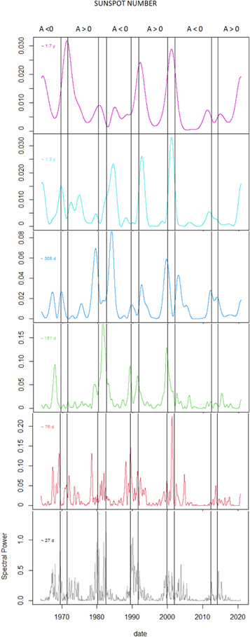
Figure 9. Temporal evolution of the spectral power of the periodicities detected in the SSN throughout SCs 20–24. The vertical lines indicate the Sun's magnetic polarity reversal interval. The intervals with positive and negative polarity are represented by A > 0 and A < 0, respectively.
Download figure:
Standard image High-resolution image
4. Conclusions
The GNM has been calculated by averaging the counting rates in typified units of the different selected NMs in each SC following the criteria of López-Comazzi & Blanco (2020).
Attending to the behavior of the SSN and the GNM along the solar cycle, a time lag of 4–6 days is obtained in the even cycles showing an almost perfect phase opposition. On the other hand, delays of 111 days and 307 days are observed in SC21 and SC23, respectively. This fact could imply certain dependency of cosmic-ray periodicities with the solar cycle polarity, specially for those periods originated by changes in the conditions of cosmic-ray propagation.
In order to compare the periodicities found in the GNM counting rates with those found in the SSN, the Morlet wavelet analysis has been applied to both of them from 1964 to 2019, i.e., covering five SCs. The periodicities detected in the GNM counting rates are: ∼13.5, ∼27, ∼46–64, ∼79–83, ∼134–190 day periods (Rieger type), ∼225–309 day periods, ∼1.06–1.15 yr periods, ∼1.3 yr periods, and ∼1.7 yr periods. The periodicities detected in the SSN were 13.5, 27, ∼46–64, 77, ∼106–124, and 141–161 day (Rieger-type), ∼239–301 day, ∼1 yr, ∼1.3 yr, and ∼1.7 yr periods.
Some of the cosmic-ray periodicities could appear as a consequence of a modulation effect related to solar dynamo and so Rossby waves, which are directly related to solar dynamo, could be the origin of them. This relationship is confirmed by the coincidence in the periods both in the GNM and the Rossby wave model. The ones possibly related to solar dynamo are 77–83 day, Rieger-type, 225–309 day, ∼1.3 yr, and ∼1.7 yr periods.
The temporal evolution of the cosmic-ray periodicities has been studied. We found that the 1.3 yr period mainly responds to changes in propagation conditions in the heliosphere because it is only detected in the even cycles. Another interesting result is obtained in relation to the 1.7 yr period. The ∼1.7 yr period shows the strongest spectral power, although the duration of the period is not constant from one SC to another and varies between 1.77 and 2.20 yr. This periodicity shows an inversely linear relationship between the average of the SSN in each SC and the corresponding period associated to the 1.7 yr periodicity. If this relationship is correct, the duration time of the ∼1.7 yr period in the SCs prior to the existence of NMs could be inferred.
The authors give thanks to the MINECO—FPI 2017 Program cofinanced by the European Social Fund. This work has been supported by the projects CTM2016-77325-C2-1-P and by the project PID2019-107806GB-I00 funded by the Ministerio de Economía y Competitividad and by the European Regional Development Fund, FEDER. Data of the NMs have been downloaded from NMDB page: http://www.nmdb.eu/nest/.
Appendix: Neutron Monitors Used in Each Solar Cycle to Build the Global Neutron Monitor
Table 6. Selected Neutron Monitor Rankings, along the SCs 20–24, According to the Quality Index Qj
| Solar Cycle 20 | |||||
|---|---|---|---|---|---|
| Station | Qj | Qu | Qx | PCP | h |
| OULU | 0.9984 | 0.9393 | 0.8209 | 1.1144 | 0 |
| MOSC | 0.9984 | 0.9301 | 0.8173 | 2.1618 | −1 |
| SNAE | 0.9979 | 0.9222 | 0.8138 | 4.9692 | 2 |
| KIEL | 0.9978 | 0.9440 | 0.8279 | 0.4917 | 0 |
| KERG | 0.9972 | 0.9235 | 0.8282 | 1.0364 | −1 |
| INVK | 0.9969 | 0.9440 | 0.8254 | 0.1269 | −8 |
| CALG | 0.9958 | 0.9351 | 0.8173 | 1.7550 | 8 |
| NEWK | 0.9956 | 0.9043 | 0.8290 | 0.8855 | 5 |
| MCMU | 0.9951 | 0.8823 | 0.8254 | 1.2953 | 0 |
| APTY | 0.9950 | 0.8776 | 0.8092 | 3.4970 | 0 |
| HRMS | 0.9923 | 0.9327 | 0.7988 | 1.4232 | −1 |
| THUL | 0.9917 | 0.8302 | 0.8235 | 1.2313 | 1 |
| ROME | 0.9046 | 0.8329 | 0.8020 | 0.8125 | −1 |
| Solar Cycle 21 | |||||
| Station | Qj | Qu | Qx | PCP | h |
| IRKT | 0.9985 | 0.9589 | 0.8691 | 4.6012 | −4 |
| HRMS | 0.9983 | 0.9578 | 0.8741 | 0.7756 | 0 |
| NEWK | 0.9977 | 0.9544 | 0.8711 | 2.0801 | 4 |
| KERG | 0.9966 | 0.9621 | 0.8721 | 1.2676 | 0 |
| SNAE | 0.9960 | 0.9553 | 0.8652 | 2.2658 | 1 |
| OULU | 0.9955 | 0.9603 | 0.8725 | 1.3197 | 0 |
| KIEL | 0.9954 | 0.9689 | 0.8748 | 0.2031 | 0 |
| MCMU | 0.9943 | 0.9621 | 0.8697 | 1.2100 | 1 |
| JUNG1 | 0.9936 | 0.9628 | 0.8648 | 1.8205 | 0 |
| INVK | 0.9927 | 0.9529 | 0.8687 | 1.4816 | −7 |
| NVBK | 0.9897 | 0.9317 | 0.8567 | 1.0960 | −3 |
| AATA | 0.9885 | 0.9483 | 0.8557 | 1.9421 | −3 |
| LMKS | 0.9858 | 0.9226 | 0.8609 | 2.6536 | 0 |
| MOSC | 0.9854 | 0.9551 | 0.8698 | 0.4215 | −1 |
| PTFM | 0.9844 | 0.9292 | 0.8608 | 1.0297 | −1 |
| APTY | 0.9839 | 0.8599 | 0.8579 | 0.0891 | 0 |
| DRBS | 0.9821 | 0.8963 | 0.8436 | 1.3936 | 0 |
| ROME | 0.9759 | 0.9283 | 0.8660 | 0.5203 | −1 |
| Solar Cycle 22 | |||||
| Station | Qj | Qu | Qx | PCP | h |
| KIEL | 0.9998 | 0.9910 | 0.9030 | 1.0860 | 0 |
| MOSC | 0.9996 | 0.9898 | 0.9025 | 0.3187 | −1 |
| NEWK | 0.9994 | 0.9869 | 0.9008 | 0.3934 | 1 |
| MGDN | 0.9994 | 0.9888 | 0.9001 | 3.1371 | −3 |
| INVK | 0.9994 | 0.9893 | 0.9007 | 1.2010 | 0 |
| KERG | 0.9993 | 0.9912 | 0.9015 | 0.2025 | 0 |
| THUL | 0.9993 | 0.9900 | 0.9010 | 0.5844 | 0 |
| OULU | 0.9991 | 0.9901 | 0.9023 | 1.5300 | 0 |
| CLMX | 0.9990 | 0.9847 | 0.9011 | 3.3522 | 0 |
| HRMS | 0.9989 | 0.9875 | 0.9004 | 1.1331 | −1 |
| TERA | 0.9988 | 0.9910 | 0.9002 | 0.1829 | 0 |
| MCMU | 0.9988 | 0.9897 | 0.8993 | 0.3025 | 0 |
| NVBK | 0.9988 | 0.9893 | 0.8956 | 0.3980 | −3 |
| APTY | 0.9986 | 0.9902 | 0.9016 | 0.2002 | 0 |
| CALG | 0.9981 | 0.9758 | 0.8991 | 0.7489 | 0 |
| YKTK | 0.9981 | 0.9815 | 0.8997 | 4.6211 | −2 |
| DRBS | 0.9977 | 0.9663 | 0.8809 | 2.3111 | 0 |
| SOPO | 0.9965 | 0.9892 | 0.8947 | 1.3091 | 1 |
| LMKS | 0.9947 | 0.9650 | 0.8931 | 0.8996 | −1 |
| JUNG1 | 0.9945 | 0.9738 | 0.8919 | 2.6884 | 0 |
| PTFM | 0.9933 | 0.9885 | 0.8921 | 1.3828 | −1 |
| ROME | 0.9930 | 0.9835 | 0.8960 | 0.9928 | −1 |
| Solar Cycle 23 | |||||
| Station | Qj | Qu | Qx | PCP | h |
| HRMS | 0.9998 | 0.9679 | 0.8642 | 1.4678 | 0 |
| NEWK | 0.9994 | 0.9615 | 0.8662 | 0.9684 | 3 |
| CALG | 0.9994 | 0.9570 | 0.8534 | 1.5122 | 6 |
| MOSC | 0.9989 | 0.9650 | 0.8613 | 0.7159 | −1 |
| KIEL | 0.9986 | 0.9613 | 0.8619 | 2.8884 | 0 |
| MGDN | 0.9984 | 0.9625 | 0.8644 | 0.9545 | −6 |
| JUNG1 | 0.9983 | 0.9542 | 0.8652 | 0.9369 | 0 |
| OULU | 0.9982 | 0.9660 | 0.8683 | 0.7316 | 0 |
| NVBK | 0.9980 | 0.9502 | 0.8566 | 0.2858 | −3 |
| THUL | 0.9974 | 0.9593 | 0.8618 | 0.9323 | 1 |
| MCMU | 0.9971 | 0.9610 | 0.8658 | 1.4151 | 1 |
| APTY | 0.9961 | 0.9385 | 0.8596 | 0.1424 | 0 |
| INVK | 0.9958 | 0.9594 | 0.8651 | 2.5943 | 0 |
| PTFM | 0.9943 | 0.9287 | 0.8543 | 0.9989 | −1 |
| ROME | 0.9943 | 0.9577 | 0.8547 | 1.0155 | −1 |
| DRBS | 0.9779 | 0.8148 | 0.8131 | 1.8988 | 0 |
| JUNG | 0.9722 | 0.8604 | 0.8289 | 1.0682 | 0 |
| Solar Cycle 24 | |||||
| Station | Qj | Qu | Qx | PCP | h |
| NAIN | 0.9991 | 0.9386 | 0.7928 | 1.8949 | 4 |
| KERG | 0.9989 | 0.9354 | 0.7943 | 3.9648 | −1 |
| TERA | 0.9989 | 0.9247 | 0.7878 | 2.7217 | −4 |
| OULU | 0.9988 | 0.9414 | 0.7966 | 1.0725 | 0 |
| MRNY | 0.9981 | 0.9206 | 0.7709 | 2.1563 | −1 |
| APTY | 0.9973 | 0.9111 | 0.7921 | 0.1458 | 0 |
| FSMT | 0.9940 | 0.9083 | 0.7835 | 1.7502 | 8 |
| NVBK | 0.9898 | 0.8770 | 0.7763 | 1.8859 | −4 |
| THUL | 0.9876 | 0.8984 | 0.7730 | 1.0658 | 4 |
| MOSC | 0.9863 | 0.8608 | 0.7848 | 0.4409 | −1 |
| NEWK | 0.9838 | 0.8833 | 0.7550 | 0.6743 | 4 |
| PSNM | 0.7830 | 0.7643 | 0.6212 | 4.3126 | −7 |
Note. The values of Qx and Qu for these stations are also presented and in all cases they exceed the value of 0.5. PCP is the percentage of corrected points by linear interpolation and h is the delay of each station with respect to OULU.