


Abstract
Magnetic helicity is a measure of the entanglement of magnetic field lines used to characterize the complexity of solar active region (AR) magnetic fields. Previous attempts to use helicity-based indicators to predict solar eruptive/flaring events have shown promise but not been universally successful. Here we investigate the use of a quantity associated with the magnetic helicity, the magnetic winding, as a means to predict flaring activity. This quantity represents the fundamental entanglement of magnetic field lines and is independent of the magnetic field strength. We use vector magnetogram data derived from the Helioseismic Magnetic Imager (HMI) to calculate the evolution and distribution of the magnetic winding flux associated with five different ARs, three of them with little flaring activity/nonflaring (AR 11318, AR 12119, AR 12285) and two highly active with X-class flares (AR 11158, AR 12673). We decompose these quantities into "current-carrying" and "potential" parts. It is shown that the ARs that show flaring/eruptive activity have significant contributions to the winding input from the current-carrying part of the field. A significant and rapid input of current-carrying winding is found to be a precursor of flaring/eruptive activity, and, in conjunction with the helicity, sharp inputs of both quantities are found to precede individual flaring events by several hours. This suggests that the emergence/submergence of topologically complex current-carrying field is an important element for the ignition of AR flaring.
Export citation and abstract BibTeX RIS

Original content from this work may be used under the terms of the Creative Commons Attribution 4.0 licence. Any further distribution of this work must maintain attribution to the author(s) and the title of the work, journal citation and DOI.
1. Introduction
One of the most important problems in solar physics is to differentiate the magnetic field configurations in active regions (ARs) that will lead to flaring events and coronal mass ejections (CMEs) from those that will not. A significant number of teams have developed methods aiming to predict AR flaring and CME activity based on magnetogram data (see Guennou et al. 2017; Leka et al. 2019a, 2019b). A recent collaborative effort to cross-compare forecasting methods published a number of papers discussing the means for comparing and testing the efficacy of some of the established predictive tools currently available (Barnes et al. 2016; Leka et al. 2019a, 2019b; Park et al. 2020b). A particular (and significant) subset of these methods relevant to our work is termed "Magnetic/Modern Quantification" in Leka et al. (2019a) and involves the calculation of scalar measurements or proxies for the free magnetic energy of the system (which implies the existence of magnetic helicity Berger 1993; Aly 2014). Alternative methods also use machine-learning techniques or regression-based methods to assess the importance of multiple parameters across historical data. The results detailed in Leka et al. (2019a, 2019b) indicate that the methods (across all classes) do show intelligence (in a statistical sense) but that they are still not consistently reliable.
Guennou et al. (2017) conducted a test of many of the suggested metrics from the magnetic/modern quantification literature: more than 90 such scalar diagnostics. They categorized them, approximately, as those that are magnetically based: estimators of the field's structure (and hence energy), such as shear angles (a difference form a potential field) and inclination angles (angles of the field); measures of magnetic flux; current properties, e.g., net positive current; measures of (Lorentz) forces; properties of the magnetic polarity inversion line (MPIL), e.g., lengths of the line with certain properties and field/current gradients in its vicinity; and other quantities such as the helicity flux and direct estimations of the free energy. The MPIL properties are found to perform best in Guennou et al. (2017), but as we see in Leka et al. (2019a, 2019b), any performance is not optimal when applied to real data. As we now discuss, work subsequent to this has indicated that the magnetic helicity could be a crucial quantity in advancing accuracy of magnetic/modern predictive techniques.
Magnetic helicity is a fundamental quantity of magnetohydrodynamics (MHD). It is a conserved quantity in ideal MHD, and even in the limit of small or vanishing dissipation (Berger & Field 1984; Faraco & Lindberg 2020; Faraco et al. 2022). Magnetic helicity has a topological interpretation in terms of the average linking number of the magnetic field lines weighted by the field strength (Arnold & Khesin 1999; Berger & Field 1984; Prior & Yeates 2014). The use of magnetic helicity as a diagnostic tool in the analysis of solar ARs has led to significant progress in the understanding of the structural evolution of the magnetic field in ARs (e.g., Pariat et al. 2006; Pariat et al. 2005; Nindos et al. 2003; Liu & Schuck 2012; Knizhnik et al. 2015; Priest et al. 2016; Pariat et al. 2017; Zuccarello et al. 2018; Vemareddy 2019; Liu et al. 2019; Wang et al. 2018).
Concerning helicity estimations purely from observational data, Park et al. (2020a, 2021) calculated helicity fluxes for snapshots of AR temporal evolution across a wide range of locations on the solar disk. The aim was to analyze how closely the sign of the helicity flux fits the hemispherical helicity hypothesis (positive helicity in the southern hemisphere, negative in the north). What is of particular interest in this study is the second paper, Park et al. (2021), in which it was found that a number of regions not satisfying the hypothesis where those with the strongest flaring activity, particularly complex regions like AR 12673, implying that the complexity of the region may be a contributory factor to flaring activity.
Korsós et al. (2020) studied the wavelet decomposition of helicity input time series for both flaring and nonflaring ARs. This study focused on a smaller set of ARs (six in total), calculating continuous helicity time series for each region. They found some evidence that the regions that had significant flaring activity had more short-lived helicity-rich magnetic structures (termed periodic structures in the paper) than those without flaring, suggesting the potential for the development of predictive methodologies from observational magnetogram data alone through analysis of the helicity flux.
A number of other authors have investigated observationally derived helicity fluxes for AR data. Some found that shearing (fluid) motions at the photosphere account for a significant portion of helicity injected into an AR (Wang et al. 2018; Li et al. 2019; Guo et al. 2013; Liu et al. 2014). Others find evidence that preemerging twist plays a dominant role in helicity injection (Nindos & Zhang 2002; Luoni et al. 2011; Poisson et al. 2015). There are a number of other studies that look at various other properties of observational helicity injection (Jeong & Chae 2007; Yang et al. 2009; Tian & Alexander 2009; Yamamoto & Sakurai 2009; Chandra et al. 2010; Liu & Schuck 2012; Park et al. 2012; Vemareddy et al. 2015; Vemareddy 2019). However, none of these are directly attempting to demonstrate a direct predictive link between helicity flux and AR flaring, so we do not discuss them at length here.
A second strand of research has been the use of magnetic helicity as a magnetic quantification method when twinned with models of the magnetic field in the lower solar atmosphere. This method has led to varying degrees of success, but recent studies indicate that there is some potential in the method. Pariat et al. (2017) (see also Zuccarello et al. 2018) tested various quantities based on magnetic helicity, for their predictive capability, against a variety of eruptive and noneruptive magnetic flux emergence simulations (no observational data were used for these studies). One particular metric successfully indicated the onset of eruptions in MHD simulations. This quantity, referred to as the helicity eruptive index, is based on a particular decomposition of magnetic helicity. Briefly, in a simply connected domain Ω, the relative helicity HR of two magnetic fields B (the main magnetic field) and B P (a reference magnetic field), which satisfy B · n = B P · n on ∂Ω (with unit normal vector n on ∂Ω), is

where A and A P are the vector potentials of B and B P , respectively. The subscript P is used for the reference field, as this is often taken to be a potential field (though this is not strictly necessary). Following Berger (1999), Equation (1) can be decomposed into two gauge-invariant parts, HR = H1 + H2,


The first quantity, H1, is clearly the classical helicity of the closed field B − B P and thus represents the contribution due to the current-carrying part of the field. The second quantity, H2, has no clear interpretation since A P is not a closed vector field in Ω. However, it can be thought of as a measure of the mutual linkage of the current-carrying field and the (potential) reference field.
The ratio ∣H1/H2∣ is referred to as the helicity eruptive index and has been shown to give consistent results in predicting CME-like eruptions in flux emergence simulations (Pariat et al. 2017) and coronal simulations with a driven lower boundary (Zuccarello et al. 2018). This metric has shown some potential as a predictor of eruptions in observations, where the magnetic field is constructed by extrapolations from real AR magnetogram data (Moraitis et al. 2019; Thalmann et al. 2019b), However, despite some success, the eruptive index has not been found to be consistent across a wider range of AR extrapolations (Gupta et al. 2021). In a related study Tziotziou et al. (2012) studied 43 ARs using nonlinear force-free extrapolations, covering both eruptive and noneruptive ARs, and showed that the correlation between relative helicity and magnetic free energy is monotonically increasing and significantly correlated. There is some tentative evidence that by computing their relative helicity/free energy budgets we might be able to predict the potential for CME/eruptive activity of the region. The relative helicity was not, however, found to consistently predict eruptive behavior in Pariat et al. (2017).
In a similar vein, Pagano et al. (2019) developed an eruptive index for magnetofrictional simulations of an AR's magnetic field evolution, derived from magnetogram data. This eruptive index is based on a proxy for identifying a flux rope and measures the balance of Lorentz forces pushing up and pinning down this structure. So while not explicitly related to helicity, it can be seen to be based on a similar principle of identifying a region of coherent current-carrying field and the relative pinning/entanglement of this field by the background field. Again this metric has shown significant promise in some ARs (dominantly bipolar), but it is not consistent across a wider range of regions (Yardley et al. 2021). The issues with these methods are, in part, due to the need for a particular model in order to create the three-dimensional magnetic field. Yardley et al. (2021) discuss the effect of the accuracy of their magnetofrictional extrapolations on the accuracy of the prediction, which is found to be significant. Similarly, Thalmann et al. (2019a) discuss the significant effect of various model constraints on the value of the estimated helicity of the field. A final interesting example of the effect of modeling on predictive capability was introduced in Kusano et al. (2020). The flare prediction index is the ratio of the magnetic twist in a localized subset of field lines from a nonlinear field extrapolation and the flux of the field that is overarching this twisted field. One of the regions analyzed in their work, AR 12673, will be studied here from the point of view of topological changes captured by magnetic winding (see later), providing complementary insight into the region's remarkably intense flaring nature. In a follow-up paper, Lin et al. (2021) investigated the method for the identification of twisted flux ropes and their overlying field. Interestingly, the metric was found to perform better when the flux rope region was identified from the location of flare ribbons in observational data rather than in the model itself. We would add that typical quasi-static modeling methods, used in conjunction with observations, have the potential to introduce error, as the assumptions made in extrapolations, such as the field being in equilibrium and the force-free assumption holding at the photosphere, likely do not apply in practice. For all these reasons, in this work we instead focus on the topological information that can be obtained from magnetogram data without the need for a three-dimensional extrapolation. By taking this approach, we hope to avoid the layer of uncertainty introduced by three-dimensional models. That being said, the approach adopted in extrapolation-based approaches, namely, the identification of current-carrying and potential parts of the AR field, will be crucial to our work.
In summary, there is still a pressing need for the further development of flaring/CME predictive metrics, and there is significant promise shown by methods that look at the decomposition of the magnetic field into a current-carrying component and a potential component. Further, quantification of the magnetic field's developing topology is an efficient way to characterize this split. Here we present the analysis of magnetic winding as a diagnostic tool in the characterization of the developing magnetic field topology in AR. Magnetic winding is a renormalization of magnetic helicity that removes the magnetic flux weighting, thus leaving a direct measure of field-line topology (Prior & MacTaggart 2020; MacTaggart & Prior 2021a). As such, magnetic winding is more sensitive to topological changes in the magnetic field configurations than the helicity. In previous studies of magnetic flux emergence simulations, magnetic winding was shown to be a valuable tool in the characterization of field-line topology (MacTaggart & Prior 2021a). In particular, it was shown in MacTaggart & Prior (2021a) that winding can identify the preexisting twisted nature of the emerging field, while the helicity presents an ambiguous picture. This is because the helicity is significantly affected by regions of magnetic field being pulled back below the photosphere by convection (this "pulling back" is also observed in Cheung et al. 2010), presenting a temporary reversal of the helicity input. Magnetic winding, on the other hand, is less sensitive to these downflows and instead characterizes the general input of twisted field topology. More recently, MacTaggart et al. (2021) applied the magnetic winding diagnostic to observational data to present the first direct observational evidence of a dominating pretwisted structure emerging to create an AR (as opposed to twist developed only by photospheric shearing flows). This work is a crucial rationale for the predictive tools developed in this paper, as it indicates that there are ARs for which much of the current-carrying structure of the field preexists the emergence of the AR (it is formed below the photosphere). Thus, we should be able to detect this current-carrying topology from magnetogram data alone.
In the present study, we use vector magnetogram data from the Helioseismic and Magnetic Imager (HMI) of five ARs and analyze their evolution in terms of their magnetic flux, magnetic helicity, and winding. We show, by decomposing the magnetic field into potential and nonpotential/current-carrying components, that highly complex (strong winding) current-carrying fields are associated with eruptive events, while fields with winding dominated by the potential component have minimal flaring activity.
2. Basic Quantities
2.1. Magnetic Winding
Here we follow the basic presentation of Prior & MacTaggart (2020), although we focus on the interpretation of winding input through the photosphere (see also MacTaggart & Prior 2021b). Magnetic winding measures the rotation of the footpoints of a field B , in a plane, and around a point x . For example, as shown in Figure 1(a), the point coincides with a point where the field line x intersects the photosphere. This point makes an angle Θ( x , y i ) with two points at which a second field line y intersects the plane. As the field evolves/emerges, these points will move, causing the angle Θ to rotate, the net change in the angle being its winding. There are two main ways this winding can come about (assuming that the curves follow ideal MHD). First, the curve can rotate following the plasma motion in the plane; we will call this braiding motion (it is also sometimes referred to as shearing motion; e.g., Liu & Schuck 2012 and Wang et al. 2018), and a representation of this motion is given in Figure 1(b). Second, if the field line has preexisting entanglement, its vertical rise (emergence) through the plane will lead to motion of its footpoints, and this will also change the angle, as shown in Figure 1(b).

Figure 1. Depictions of the winding measure and its contributions. (a) A pair of curves x and y pierce a plane (the photosphere). A footpoint of x makes angles Θ( x , y 1) and Θ( x , y 2) with two points y 1 and y 2, the winding angles. (b) We see how braiding motion (in-plane plasma motion), here represented by two rotational flows around a curve x 's footpoints, causes the curve y to wrap around x from time t0 to t2. This changes the winding angle Θ( x , y (t)) of the curves as shown. (c) The field line y has a vertical plasma velocity vz , so the twisted field line y emerges through the surface. This leads to an apparent in-plane motion of the field line, the emergence velocity, which leads to a change in the angle Θ( x , y (t)). Note, in general, that the point(s) of intersection of x would also be in motion, thus changing the angle as well.
Download figure:
Standard image High-resolution imageMore formally, we label (x1, x2) and (y1, y2) as the in-plane coordinates of points x (t) and y (t), which evolve owing to the motion of the field lines intersecting the plane at these points. Their mutual angle is

As the field evolves, the field-line intersections of the points x (t) and y (t) will change. The time derivative of this angle is
The vector u ( y ) = (d y1/d t, d y2/d t) is the field line y 's in-plane footpoint motion (similarly u ( x ) for the point x ). If we write r = y − x , then Equation (5) can be written in vector form as

where  is the unit normal to the plane. The velocity
u
can then be decomposed into braiding and emergence terms
is the unit normal to the plane. The velocity
u
can then be decomposed into braiding and emergence terms
where v ∥ and B ∥ are the in-plane components of the plasma velocity and magnetic field, respectively, and vz and Bz are their out-of-plane components (Démoulin & Berger 2003). The total winding rate of the field around the field line at the point x would be

Finally, the magnetic winding rate  accounts for the vertical orientation of the field by multiplying by an indicator function σ(
y
),
accounts for the vertical orientation of the field by multiplying by an indicator function σ(
y
),

Thus, we have
We can also define the total magnetic winding d L/d t by integrating over all x ,
The averaged winding quantity d
L/d
t can hide a great deal of spatially varying information, especially in the complex fields we will consider. Therefore, we shall develop some subtler methods combining the information from the distributions  in this study.
2.2. Magnetic Helicity
We will define the magnetic helicity here as the flux-weighted winding. Thus, the field-line helicity input rate  is
is
and the total helicity input is
Note that σ and Bz have the same sign. This "definition" of the helicity is formally equivalent to the standard presentation in terms of vector potentials (technically the relative helicity in this case) as demonstrated in detail in Prior & MacTaggart (2020). To be absolutely clear: although this magnetic helicity is the same quantity that is calculated in almost all observational helicity studies, the presentation given here serves to highlight its relationship to the magnetic winding and its underlying geometrical basis.
2.3. Helicity and Winding Fluxes: Basic Comparisons
The clear difference between helicity and winding fluxes is the magnetic flux weighting. In effect, this acts to bias the helicity calculation toward winding associated with field components with high values of Bz . In practice, in AR data, this means prioritizing contributions from the field in the locality of the sunspots, as highlighted in MacTaggart et al. (2021; see also the examples in Figures 2(a) and (b)). We should be clear, however, that it does not mean a bias toward overall stronger field. The evidence from geometrical experiments (Prior & MacTaggart 2020), flux emergence experiments (Prior & MacTaggart 2019; MacTaggart & Prior 2021a), and observational data (MacTaggart et al. 2021) is that the winding input is dominated by regions of strong field where the field is significantly transverse (∣ B ∣ is (relatively) large, but Bz is not). Typically, this occurs in the region between the main spots where the polarity inversion line resides (see Figure 2(c)). In the AR considered in MacTaggart et al. (2021), it was found that both the helicity and winding are dominated by field components whose strength is between 100 and 200 G, but in different locations (at the sunspots and between them, respectively).

Figure 2. Typical AR locations of helicity and winding fluxes. Panel (a) is the Bz magnetogram snapshot for AR 11318 during the development of its bipole structure. Panel (b) represents the helicity flux for this region; the contours of 400 G indicate that the dominant contributions arise in the locality of the magnetic poles. Panel (c), by contrast, shows the winding flux, which is dominantly in between the magnetic poles in the region where the polarity inversion line resides.
Download figure:
Standard image High-resolution imageIntriguingly, the results presented in Lin et al. (2021), extending those of Ishiguro & Kusano (2017) and Kusano et al. (2020), provide a potential insight as to why the magnetic winding might provide important information regarding flaring/CME activity. In that work, an eruptivity index for an extrapolated field was calculated for two sets of field lines. The first were those whose anchoring points were selected from the location of the observed flare ribbons. These field lines emanated from between magnetic poles (where we see that the winding flux tends to accumulate). The second were those whose local twisting values were maximal, in which case the field lines were anchored at the poles. The metric was found to perform better when the field lines in between the poles were used (those based on the flare ribbon location). Of course, this determination could not be properly predictive, as it requires flare ribbon data. We will show in this work that magnetic winding, which can dominate at the polarity inversion line, has significant potential for predicting flaring activity.
2.4. Potential−Current Decompositions
A magnetic field (in a simply connected domain) can always be split into a part that is potential
B
p
and a part that has current
B
c
(the Helmholtz decomposition). We can apply this idea to magnetogram data as follows. The Bz
distribution can be used to determine a potential field assuming periodicity as detailed in Prior & Berger (2012) (with α = 0) (this periodic assumption should be reasonable for Space-Weather HMI Active Region Patches (SHARP) data, which tend to surround the AR with layers of negligible field strength). This simply requires that we obtain the Fourier transform of the Bz
distribution, from which the in-plane components of  can be obtained. Then, we can define a field
B
c
as
B
c
=
B
−
B
p
, which we refer to as the current-carrying field. This field is two-dimensional, with no component orthogonal to the photospheric plane. Using this decomposition, we can write the field-line velocity as
can be obtained. Then, we can define a field
B
c
as
B
c
=
B
−
B
p
, which we refer to as the current-carrying field. This field is two-dimensional, with no component orthogonal to the photospheric plane. Using this decomposition, we can write the field-line velocity as

where we have an emergence velocity due to the potential part of the field and emergence velocity due to the motion due to the current-carrying part (note that B c ≡ B ∥c ). We can then decompose the winding and helicity by these motions. In particular, we will define a kernel

where u 1 and u 2 represent particular velocity components that are being studied (see below for details). Based on this kernel K, we can define the following winding quantities:


To keep the notation as clear as possible, we provide the following table of shorthand labels: both symbolic labels and names to be used in the text.
| u b = v ∥ |

| braiding velocity/braiding winding |

|

| emergence velocity/emergence winding |

|

| potential velocity/potential winding |

|

| current-carrying velocity/current-carrying winding |
Download table as: ASCIITypeset image
For example, the braiding winding flux is written as

Note that since the winding and helicity calculations are linear in the decomposition of u , the following identities hold:

and similarly,

The subtraction is necessary, as both current-carrying and potential measures account for the plasma velocity motion. We can also do the same for helicity-like quantities,


A similar labeling will apply to the decomposed component of the helicity, e.g., He is the emergence component of the total helicity.
Our definition also allows for mixed quantities like L( u c , u p ), a measure of the entanglement of the potential and current-carrying field components. We calculated these quantities but found that they did not offer any significant additional information. Therefore, for the sake of clarity, we omit these results here.
2.4.1. Current−Potential Balances
We will show that a critical factor for predicting the likelihood of flaring activity is the balance of current-carrying and potential topological input. In order to quantify this balance, we define two quantities. The first measures the temporally accumulated difference between the spatially integrated current-carrying and potential topological inputs,
For complex AR, there can be significant amounts of cancellation in the global quantities dLc/p /dt and dHc/p /dt. Therefore, we also calculate the temporally accumulated difference in the absolute local balance of these contributions,
The measures in Equation (26) will allow us to identify local regions of topological input that are precursors to flaring activity. Occasionally we will refer to plots of the time derivatives of these quantities. To avoid cumbersome notation, i.e., dδ
L/dt, we use dots to denote their time derivatives, that is,  .
.
One crucial consideration in the choice of these metrics is that we often find regions where there is little actual transversal field B ∥ but some significant potential field B ∥p . In this case, the current-carrying field would be the opposite of the potential field B ∥c − B ∥p (or close to that). In the case of very weak actual transversal field ( B ∥), we should not expect a contribution to the region's flaring activity. The absolute sign difference in these two measures (δ L and ΔL) aims to minimize such contributions, as they would be canceled directly if B ∥c = − B ∥p .
For example, we see in Figure 3(a) the distribution  for one of the fields used in this study, and in panel (b)
  at the same time. There is significant morphological similarity between the two, with the signs reversed. On cancellation in the distribution
  , shown in panel (c), we see that there is still some imbalance that favors current-carrying field. This distribution in panel (c) represents a meaningful net imbalance toward current-carrying winding at a given location in the observed field.

Figure 3. Images showing cancellations in the δ
L measure. Panel (a) is the distribution  for a given snapshot of the AR 11318. Panel (b) is the distribution
  at the same time. Panel (c) is the distribution
  at the same time. Figures are shown in a box around the center of the AR.
Download figure:
Standard image High-resolution image3. Analysis of Active Regions
In what follows we describe the evolution of the helicity and winding indicators, introduced in the previous section, for five ARs. The first three ARs, AR 11318, AR 12119, and AR 12885, show minimal or flaring activity. The other two ARs, AR 11158 and AR 12673, show significant flaring activity. All regions, except for AR 12885, have been the subject of previous analysis (e.g., Romano et al. 2014; Toriumi et al. 2014; Dacie et al. 2018; Moraitis et al. 2019), to which our results can be compared. To perform winding flux calculations, we use SHARP vector magnetograms taken by HMI on board the Solar Dynamics Observatory (Scherrer et al. 2012) with 0 5 pixel resolution and 12-minute cadence. In our analysis, we use the magnetogram data sets from AR in their full availability span, indicating in the figures times when the ARs are close to the limb and the magnetic field inversion procedure becomes more problematic. Here we use the criterion that the inversion procedure for regions between longitudes of ±60° from the central meridian can be considered reliable, as previously advocated in the literature (e.g., Bobra et al. 2014; Park et al. 2020a).
In order to calculate the 3D velocity fields associated with the plasma flows during the evolution of the ARs, we employ the differential affine velocity estimator for vector magnetograms (DAVE4VM) method (Schuck 2008). We use a 20-pixel smoothing window size for the calculations in the main text; in the Appendix we also use a 12-pixel window to gauge the effect of this choice on our results. The short précis is that, while it has a quantitative effect, it does not fundamentally alter the validity of the conclusions we draw in what follows, i.e., the qualitative results are not adversely affected.
3.1. AR 11318
3.1.1. Description of General Activity
AR 11318 was a relatively small bipolar region that was located at −15° with respect to the central meridian. Only one C-class flare and a subsequent CME event are associated with it (Romano et al. 2014). It appeared on 2011 October 11, rapidly forming a bipole (Figure 4(a)). After about 70 hr, these poles began to fragment (Figure 4(b)), prior to October 15, when a C2.3 flare was produced in association with a filament eruption. After the eruptive event, a smaller bipolar structure formed with the main initial positive pole (Figure 4(c)).
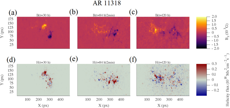
Figure 4. Magnetic field Bz (top) and helicity (bottom) distributions at three different stages of the evolution of AR 11318, t = 2 hr, t = 50 hr, and t = 84 hr.
Download figure:
Standard image High-resolution imageThe evolution of the magnetic helicity in AR 13118 was the subject of a previous study by Romano et al. (2014), which suggested that the magnetic flux and magnetic helicity are only partial indicators of the likelihood of an eruptive event. In MacTaggart et al. (2021) it was shown that this field emerged with significant preexisting twisted structure. We extend these calculations here for a longer period of time.
3.1.2. Evolution of the Basic Topological Quantities
The winding and helicity evolutions are presented in terms of their emergence/braid decomposition in Figures 5(a) and (d), respectively. In the initial phase there is a rapid input of winding that lasts about 20 hr and coincides with the development of the bipole structure seen in Figure 4(a) (note that there is a region of missing data between 20 and 30 hr that produces a false plateau). The increase in total winding is largely dominated by its emergence term, as opposed to the braiding term; see Figure 5(a) (as discussed in MacTaggart et al. 2021). This means that the initial change in the magnetic field topology in AR 11318 is mainly due to the emergence of pretwisted field, rather than horizontal braiding motion at the photosphere. After that, the rate of input of winding decreases, but it is still positive until it stabilizes at around 60 hr. The stabilization is accompanied by the maximum value of the emergence term of the winding, suggesting that most of the emergence of topologically complex magnetic field had already happened at that point. A comparison of simulations and observations carried out in MacTaggart et al. (2021) indicates that this plateauing occurs as the magnetic field expands into the solar atmosphere. At this time, parts of the magnetic field are pulled back below the photosphere by convection. This is consistent with the fracturing of the magnetic structure seen in Figure 4(b). In the later phase ≳80 hr, the net winding flux changes sign, which coincides with the restructuring and development of the new smaller bipole structure, as seen in Figure 4(c). At the initial of this reversal, there is a sharp drop in the emergence contribution at about 80 hr. The drop indicates a sudden loss of some structure. We do not focus on the exact spatial nature of the event at this stage; we will see later a similar but more significant drop in the region AR 12673.
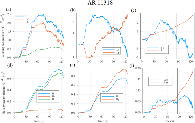
Figure 5. Top: evolution of magnetic winding accumulation of AR 11318, including (a) its emergence/braiding decomposition, (b) the potential/current-carrying decomposition, and (c) the differences between potential and current-carrying winding. Bottom: the helicity analysis of the same region, including (d) its emergence/braiding decomposition, (e) the potential/current-carrying decomposition, and (f) the differences between potential and current-carrying helicity.
Download figure:
Standard image High-resolution imageThe dominance of the emergence term of the winding is contrasted by the evolution of the magnetic helicity, to which the same decomposition is applied (Figure 5(d)). The evolution of the magnetic helicity shows that the dominant term here is the braiding and not the emergence. We can see that the spatial distribution of the helicity flux matches well with the line-of-sight magnetic flux (see the top and bottom rows of Figure 4). By contrast, we see in Figures 6(a)–(c) that the majority of the winding input arises in between the magnetic poles, where the central core of the flux rope has emerged transversally. This fact is discussed at length in MacTaggart et al. (2021), and, as discussed above, this input results from a field that is greater than 100 G but that is dominantly transverse. It is interesting here to see in Figure 6(c) that there is significant negative winding input between the newly formed bipole structure that is present at later times, suggesting a structural rearrangement after the flaring event.

Figure 6. Magnetic winding distributions at three different stages of the evolution of the AR 11318 at t = 2 hr, t = 50 hr, and t = 84 hr. The rows show the total winding (top), the potential part (middle), and the current-carrying part (bottom). Green lines represent contour sets for the vertical magnetic field Bz = 800 G.
Download figure:
Standard image High-resolution image3.1.3. Evolution of Current/Potential Decompositions
Plots of the time-integrated current-carrying/potential topological decomposition are shown in Figures 5(b) and (e). The potential and current-carrying terms of the helicity (panel (e)) remain comparable throughout the entire lifetime of this AR; this is not a surprise since the braiding/transverse velocity is not decomposed and dominates the helicity. The winding decomposition, by contrast, has a much more interesting variation. In the initial phases of the evolution of the AR, both the potential and current-carrying components of the winding are subject to a short phase of rapid increase and of opposing sign, starting at around t = 15 hr and lasting for at least 7 hr (followed by a 7 hr gap in which data are unavailable). Up to about 40 hr the magnitude of the current-carrying winding Lc rises more rapidly than Lp as the field emerges, and therefore it dominates the winding balance up to this point. This coincides with the initial stage of flux emergence (MacTaggart et al. 2021). The current imbalance, combined with the bipolar nature of the structure, is consistent with the formation of a sigmoidal structure in this region, as observed in Romano et al. (2014). After 40 hr, negative (potential) winding begins to increase rapidly, quickly turning positive, and then steadily accumulates (Figure 5(b)). By contrast, between 40 and 80 hr, the net current-carrying winding stays largely fixed. After this period, there is a drop in the current-carrying part, and they are roughly of equal value before finally rapidly growing in opposing directions with a sign inverted from the earlier input. Once again the current-carrying part grows quicker. This later growth appears to coincide with the formation of the new bipole observed in Figure 4(c).
The current−potential balance metrics ΔL, ΔH, δ L, and δ H are shown in Figures 5(c) and (e). Over the first 50 hr, for which we have seen that there is a significant input of positive winding, both ΔL and δ L show an imbalance in favor of current-carrying winding, the rise being more dramatic, initially, in ΔL. From 50 hr until the flare (marked on Figure 5(c) with a vertical line), this imbalance is reversed for the global metric ΔL, but the local comparison metric δ L continues to steadily rise, up to and beyond the time of the flare.
The helicity comparison metrics ΔH and δ H tell a similar story to the winding measures, with δ H showing a consistent increase over the region's lifetime. The gradual rebalancing of the global measure ΔH is less marked than its winding counterpart.
It is clear that both δ metrics are registering a significant increase in localized current-carrying magnetic topology over that of the potential field. We can see in the winding flux distributions ( ) shown in Figure 6(d) (potential) and (g) (current-carrying) that the distributions are dominantly positive, representing the emerging twisted field. At later times we see that the distribution of positive and negative winding is much more balanced (see Figures 6(e)−(h) and (f)−(i)), leading to significant cancellation in the global Δ measures. So it is the spatial variance between the two distributions that leads to the consistently positive δ
L measure. We can see that the location of the topological input of both measures is largely similar, so it is subtly small variances in the later stages that lead to the imbalance (see Figures 6(e)−(h) and (f)−(i)). It is particularly clear comparing Figure 6(h) to (e) that there are regions of strong winding present in the current-carrying distribution not in the potential one.
) shown in Figure 6(d) (potential) and (g) (current-carrying) that the distributions are dominantly positive, representing the emerging twisted field. At later times we see that the distribution of positive and negative winding is much more balanced (see Figures 6(e)−(h) and (f)−(i)), leading to significant cancellation in the global Δ measures. So it is the spatial variance between the two distributions that leads to the consistently positive δ
L measure. We can see that the location of the topological input of both measures is largely similar, so it is subtly small variances in the later stages that lead to the imbalance (see Figures 6(e)−(h) and (f)−(i)). It is particularly clear comparing Figure 6(h) to (e) that there are regions of strong winding present in the current-carrying distribution not in the potential one.
Finally, in Figure 7, we present the time series of the rates  and
and  . We highlight, in pink, the time interval when the AR is close to the limb (beyond 60° longitude from the central meridian) and the magnetogram data are considered to be less reliable. We calculate a moving average of the quantities, represented by an orange line, with an envelope of 3 standard deviations on either side of this moving average, both calculated in an interval [t − 10 hr, t]. The winding time series
  shows that the flare (indicated as a vertical line) is preceded by two spikes of strong positive
  that go beyond the 3 standard deviation envelope and occur about 6–7 hr prior to the event, implying that a strong input of current-carrying topology takes place just before the event. Hereafter, when we refer to a spike in the series, we always mean that it has exceeded the 3 standard deviation envelope. This is the same jump as was seen in the winding series itself (discussed above). Consistent with this is a noticeable rise in the rate
  , seen in this time period (6–7 hr before the flare). This suggests that
  and
and  are potentially useful as early warning signs of flaring activity. More evidence of this assertion will be presented later for other ARs. We notice that there are a few spikes in the time series
  early on in the AR lifetime (t ≤ 40 hr) that do not indicate any flaring events directly. This period corresponds to the initial emergence of the region and, hence, the initial input of topologically significant field into the atmosphere. It is normally later in the evolution of an AR when significant flares begin to appear. For AR 11318, the signature of a positive input of
  a day or two before the commencement of flaring is slightly obscured by the region of missing data. However, this pattern will appear again in the flare-intensive regions that we will consider later.
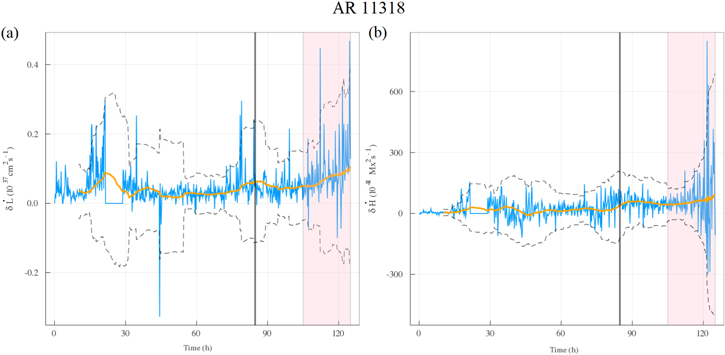
Figure 7. Time series of  and
and  for AR 11318. The C-class flare is indicated by a vertical line. The pink region indicates that the region is beyond 60°r of Carrington longitude. The orange curve is a running average of the time series, and this is bounded by an envelope of 3 standard deviations.
Download figure:
Standard image High-resolution image3.1.4. Analysis of the Effect of the Magnetic Field Cutoff and Velocity Smoothing Parameters
The calculations here depend on parameters including a cutoff of the field, 50 G, and the choice of the windowing parameter used in the DAVE4VM code, 20 pixels in this case. In MacTaggart et al. (2021), the winding/helicity calculations were performed for a variety of other field cutoffs from 20 to 400 G. It was found that there is a slight decrease in the total winding/helicity with increasing cutoff strength, up until 100 G, but that the qualitative behavior is very similar up to this value. For cutoffs greater than 100 G, there is a significant drop-off in both winding and helicity, particularly at 200 G. This result indicates that both quantities have a significant contribution from magnetic field, with a magnitude between 100 and 200 G. In the Appendix we perform similar calculations for δ L And ΔL, but we also include calculations with a smoothing in the DAVE4VM code of 12 pixels. The brief conclusion is that the distributions are qualitatively similar up to 200 G. The 12-pixel calculations tend to have a very similar qualitative shape but a higher peak value. One notable finding is that the quantity ΔL actually remains positive for 12-pixel calculations with all cutoffs but still shows significant decay from the peak value.
3.1.5. Summary and Conclusions from Region
In summary, this AR presents a single flaring event that affords a chance to provide a relatively simple analysis of the varying topological inputs that might preface such activity. We find that this flare occurs after a period of significant localized dominance of the current-carrying winding and helicity inputs, relative to the potential inputs. The differences δ
L and δ
H characterize this change and both show significant positive input (dominance of the current-carrying input) for a sustained period before the flare. The result suggests that consistent positive imbalances in these quantities might be a means for detecting automatically the onset or development of flaring activity. There are also a pair of dramatic signatures in the time series  and
and  about 6–7 hr before this event, indicating the possibility that the quantities may also be used to predict individual events.
3.2. AR 12119
3.2.1. Description of General Activity
AR 12119 was described by Dacie et al. (2018) and was a region that emerged into a larger and preexisting surrounding magnetic structure that included a large closed filament encircling AR 12119. On 2014 July 18, the bipole structure that characterized AR 12119 became clear (as seen in Figure 8(a)). As described in Dacie et al. (2018), interaction of this bipole with the preexisting filament resulted in perturbations to the existing structure that led to two CME events. Crucially, these resulted from eruptions of the preexisting filament structure, set off by reconnection with the emerging region AR 12119. It should be stressed that AR 12119 itself appeared to be a relatively simple and small AR that showed very little activity itself: no flares of magnitude C or above have been registered for this AR. We see in Figures 8(a)–(c) that it maintained a relatively straightforward bipole structure throughout its lifetime. The mechanism used to explain these eruptions is the so-called sympathetic eruption mechanism (Török et al. 2011). The analysis performed here is limited to the data associated with the SHARP data of AR 12119 alone, which exclude the overall magnetic structures around it. The aim of using only the isolated nonflaring data of AR 12119 is to compare and contrast to AR 11318, which generated its CME internally through the classic development of a sigmoidal field structure.
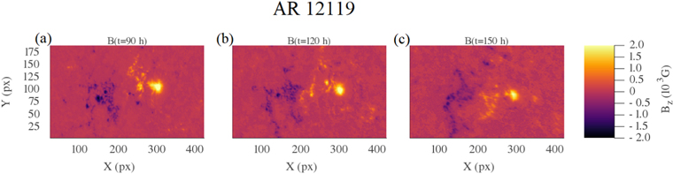
Figure 8. Magnetograms of Bz at three different stages of the evolution of AR 12119, t = 2 hr, t = 50 hr, and t = 84 hr.
Download figure:
Standard image High-resolution image3.2.2. Evolution of the Basic Topological Quantities
This region's topological inputs are shown in Figure 9, obtained by analyzing a SHARP data set beginning on 2011 October 2 at UTC 22:00:00. Similar to the AR 11318 time series, the magnetic winding accumulation (Figure 9(a)) of this AR shows a rapid increase initially, for about 120 hr. As in the case of AR 11318, the increase in the winding is largely due to vertical motions (emergence term; Figure 9(a)). The helicity signal, on the other hand, shows a dominance of the braiding term (Figure 9(b)), due to horizontal motions. Again, this difference can be attributed to the fact that the helicity input is dominated by plasma vortex motion at the sunspots (Figure 8), while the winding input is dominated by the emerging field in the region between the sunspots (Figure 10). After 120 hr, the winding input of the region levels off, again similar to AR 11318, indicating that it is expanding into the solar atmosphere rather than emerging. Toward the final stages of the observation, a strong concentration of magnetic winding is seen in the northeastern border of the region as shown in Figure 11, which is not associated with the AR's bipole. This is likely associated with the interaction of this region with the external field.
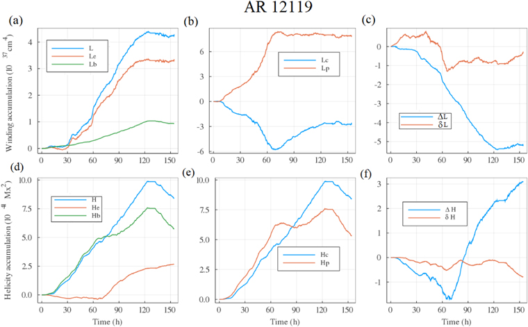
Figure 9. Evolution of magnetic winding accumulation (top) in AR 12119, including (a) its emergence/braiding decomposition, (b) its potential/current-carrying decomposition, and (c) the differences between potential and current-carrying windings. The helicity analysis (bottom) includes (d) the emergence/braiding decomposition, (e) the potential/current-carrying decomposition, and (f) the differences between potential and current-carrying helicities.
Download figure:
Standard image High-resolution image
Figure 10. Magnetic winding distributions at two different stages of the evolution of AR 12119 at t = 90 hr and t = 120 hr. The potential (top) and current-carrying (bottom) parts are displayed. Green lines represent contour sets for the vertical magnetic field Bz = 800 G.
Download figure:
Standard image High-resolution image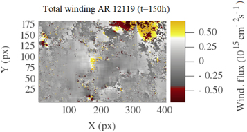
Figure 11. Magnetic winding distribution of AR 12119 at t = 150 hr showing magnetic field structure due to the interaction with another AR on the northeastern border of the box.
Download figure:
Standard image High-resolution image3.2.3. Evolution of Current/Potential Decompositions
The evolution of the potential and current-carrying components shows inputs with similar morphology but with opposite sign, similar to the early-stage evolution of AR 11318. Unlike AR 11318, however, their net values level off rather than show the dramatic changes associated with the later-stage development of AR 11318. We see in the winding distributions of these quantities, Figures 10(a), (b), (c), and (d), that this similarity is mirrored in very similar (but opposing sign) winding distributions, indicating that much of the current-carrying structure does not (generally) coincide with actual strong observed (transverse) field (as discussed above). Both quantities grow in amplitude up to ∼70, hr followed by a stabilization for the potential component, but a modest decrease in the case of the current-carrying component (Figure 9(b)). This is indicative of a gradual trend toward more potential field structure. This gradual buildup in the dominance of the potential component of the magnetic winding is highlighted by the negative values of ΔL throughout the sunspot's lifetime (Figure 9(c)). The quantity δ L shows small but positive values in the first 60 hr and then becomes negative. This lack of a buildup in positive δ L or ΔL indicates that there is no tendency toward an imbalance in current-carrying topology over potential. This is consistent with the absence of flaring activity attributable to the region per se.
The decomposition of the helicity shows that both potential and current-carrying components remain comparable up to about 90 hr, after which the current-carrying component continues to grow while the potential component stabilizes. ΔH (Figure 9(f)) is negative at the start and becomes positive after 90 hr. δ
H, on the other hand, remains slightly negative throughout the evolution of this AR. The δ signature is more consistent with the region's observed lack of intrinsic flaring activity. The rates of change of both  and
and  are analyzed in Figure 12. The fact that the emergence of this AR is dominated by potential structure is revealed by the moving average of
  with a negative tendency (Figure 12). Although a few positive spikes in the rate go beyond the 3 standard deviation envelope, none occur in a period when the accumulated current-carrying topological structure δ
L is positive (see Figure 9(c)). In addition, the absolute magnitude of the signal is smaller than what was observed for AR 11318 (typically by about a factor of 4 for the positive spikes in
with a negative tendency (Figure 12). Although a few positive spikes in the rate go beyond the 3 standard deviation envelope, none occur in a period when the accumulated current-carrying topological structure δ
L is positive (see Figure 9(c)). In addition, the absolute magnitude of the signal is smaller than what was observed for AR 11318 (typically by about a factor of 4 for the positive spikes in  ). The combination of an accumulation of potential-dominated magnetic topology and a small amplitude signal correlates with a lack of any significant intrinsic flaring.

Figure 12.
 and
and  time series for AR 12119. The format of Figure 7 is used here.
Download figure:
Standard image High-resolution image3.2.4. Summary and Conclusions from Region
AR 12119 is a relatively small bipolar AR that has attracted some interest as a trigger of "sympathetic CME eruptions." This means that this bipolar region emerged in an area with preexisting magnetic structures, and the interaction of the bipole with the preexisting filaments, and not the AR by itself, generated eruptions in the form of CMEs. The evolution of the topological quantities shows a dominance of the emergence term, similar to AR 13118, indicating a preexisting topological structure emerging. By contrast to AR 11318, the potential/current-carrying decomposition of the winding shows an overall dominance of the potential component, except for a slightly positive phase in the beginning of this AR's lifetime, which indicates that insufficient current-carrying topological structure is injected/developed in order to generate flaring/CME activity internal to the region.
Therefore, there is some tentative evidence, based on the two example regions analyzed so far, that it is the localized balance of current-carrying to potential winding/helicity (δ L and δ H) that provides a reliable indication of the likelihood of flaring activity. Crucially, it can indicate both a tendency toward flaring activity (consistent positive buildup in δ L and δ H) and a lack of flaring activity (no consistent buildup in δ L and δ H).
3.3. AR 12285
We now analyze AR 12285, a region that produced no flares of magnitude C or above. We found no detailed study of this region in the literature; however, we include it here as an example of a nonflaring region that was not subject to any significant interaction with surrounding magnetic structure (as was the case for AR 12119). We keep the description of the helicity/winding behavior of this region relatively succinct, as it is very similar to that of AR 12119. AR 12285 emerged on the disk on 2015 November 26. This bipolar region maintained its configuration, approximately, throughout its lifetime, lasting for about 3 days (see Figures 13(a), (b), and (c)).
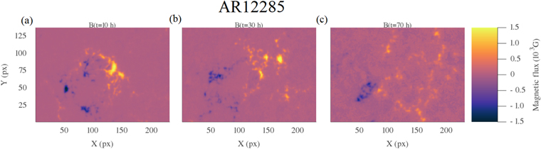
Figure 13. Evolution of Bz for AR 12855.
Download figure:
Standard image High-resolution imageThe evolution of the total winding L(t) is presented in Figure 14(a). It goes through a phase of rapid increase between 5 and 30 hr, followed by a decrease, lasting until ≈45 hr, before increasing again. Initially, the winding is dominated by the emergence term until later in its evolution, when there is a significant increase in the braiding contribution accounting for the latter rise. The current-carrying and potential components of L (Figure 14(b)) approximately reflect each other about the x-axis, with the magnitude of the potential component being slightly larger. The absolute values of the winding measures are 5–6 orders of magnitude smaller than what was observed for AR 11318 and AR 12119. ΔL is mostly negative, except in the initial emergence phase. δ
L is zero or negative until ∼45 hr. Even when it becomes positive, its magnitude is an order of magnitude smaller than those of AR 11318 and AR 12119. The behaviors of the helicity decompositions are shown in Figures 14(d)–(f). The helicity, similar to the winding, goes through a phase of rapid increase up to ≈20 hr, followed by a plateau and a decreasing phase up to ≈45 hr when it starts growing again (Figure 14(d)). The helicity is dominated by the braiding term. The potential/current-carrying decomposition shows a dominance of the potential part (Figure 14(e)), which is also evidenced by the delta measures in Figure 14(f). Here δ
H is always negative, and, except initially, so is ΔH. We do not examine the  or
or  time series, as there is never a buildup of current-carrying topology for it to be meaningful, a fact borne out by the absence of flaring activity in the region.
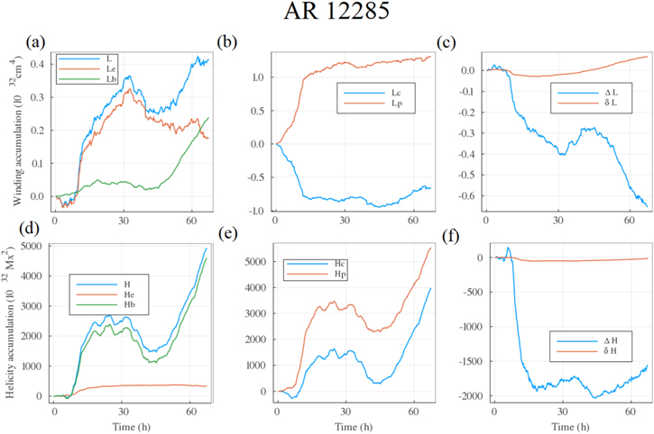
Figure 14. Evolution of magnetic winding accumulation (top) in AR 12855, including (a) its emergence/braiding decomposition, (b) its potential/current-carrying decomposition, and (c) the differences between potential and current-carrying windings. The helicity analysis (bottom) includes (d) the emergence/braiding decomposition, (e) the potential/current-carrying decomposition, and (f) the differences between potential and current-carrying helicities.
Download figure:
Standard image High-resolution image3.4. AR 11158
3.4.1. Description of General Activity
We now analyze two ARs with very prolific flaring profiles. First, we analyze AR 11158, which appeared in the southern hemisphere on 2011 February 9, lasting around 11 days. This AR yielded one X-class flare, five M-class flares, and tens of C-class flares. We will focus on the larger flares here for the sake of clarity. The region comprised two (initially) distinct bipoles. The first bipole appeared in the southern hemisphere on February 9, the second on February 10 (see Figure 15(a)). After this, the elements of both bipolar systems gradually separated from their counterparts, and the interior poles rotated around each other (Figure 15(b)). This rotation created a highly sheared polarity inversion line (PIL) and led to the significant interaction and merging of the two regions (see Figures 15(b) and (c)). This development was, as mentioned above, accompanied by a significant number of flaring events.

Figure 15. Magnetograms of Bz at three different moments of the evolution of AR 11158.
Download figure:
Standard image High-resolution image3.4.2. Previous Studies of This Region
AR 11158 has a significant history of being analyzed. Toriumi et al. (2014) conducted magnetic flux emergence simulations to test hypotheses of its development, stating that its likely development was from a pair of buoyantly rising deformations of a single large monolithic flux tube beneath the photosphere. Hayashi et al. (2018) conducted a magnetogram-driven MHD simulation of the region. Their simulation indicated that the energy release associated with the region could not be inferred form the photospheric data, a claim we dispute here, as the helicity/winding time series will indicate that some of the flaring events could have been anticipated from these data alone. Vemareddy et al. (2015) analyzed the vertical current distributions of the field, noting that there were two subregions of activity with opposite chirality: one dominated by sunspot rotation producing a strong CME, the other showing large shear motions producing a strong flare. Their conclusion was that this current flux can be explained by the emergence of a twisted flux rope in line with the conclusions of Toriumi et al. (2014). Kazachenko et al. (2015) estimated the inputted energy in this region before its X-class flare, finding significant free energy but that their was approximately four times as much energy associated with the potential field. Sorriso-Valvo et al. (2015) applied a spectral analysis to the development of the current density and helicity of the region. Sudden changes in the spectra of these distributions correlated with the occurrence of flaring events, suggesting at least some indication that energetic events can be found in magnetogram data. Tziotziou et al. (2013) calculated the energy and relative helicity budgets in this region, suggesting that a substantial amount of accumulated energy/helicity led to the eruptive phase of the AR. They also found decreases in helicity and free energy before major flare/CME events. Li & Liu (2015) observed that the maximal sunspot rotation event coincided with one of the M-class flaring events. Zhao et al. (2014) analyzed the development of the squashing factor (a measure of the divergence of initially localized field lines) in nonlinear force-free field extrapolations. This analysis indicated the formation of strong quasi-separatrix layers (indicative of the formation of sheared PILs) shortly before two of the larger flaring events. Jing et al. (2012) used similar extrapolations to analyze the development of the current helicity and magnetic helicity. Before two of the flaring events, they find suggestive bumps in the helicity distribution. Thalmann et al. (2019b), by contrast, find that the total relative helicity has little clear predictive capability, but that the eruptive index mentioned in the Introduction shows some predictive capability for two of the events (however, it is not so successful in another region). We now proceed to apply our analysis to this region. In passing, we note that the predictive capabilities mentioned above mostly arise from reconstructions of the field, not the magnetogram data alone. We find, in what follows, some predictive capability from the magnetogram data alone.
3.4.3. Evolution of the Basic Topological Quantities
We analyze the SHARP data set beginning on 2011 February 10 at 22:00:00 UTC. After a period of relatively little topological development, the winding input (Figure 16(a)) shows an initial sharp (positive) rise from about 50 to 85 hr. This is indicative of the rapid emergence of the field, similar to the initial input phase of AR 11318 (Figure 5(a)). The emergence component of the magnetic winding is dominant, indicating the rapid emergence of preexisting magnetic topology. By contrast to the winding plateau seen in AR 11318, here the input of emergence-dominated winding persists throughout the lifetime of the region's development, indicating that complex magnetic topology of a consistent chirality is being inputted into the system. The helicity input (Figure 5(b)) shows a steady rise from about 50 to 140 hr that is largely dominated by the braiding input, consistent with the sunspot rotation discussed in the existing literature about this region. The emergence term shows a significant increase in the later evolution of the field (we will see that this has consequences for flaring activity). After 140 hr, the braiding helicity input begins to reverse its sign, meaning that the net helicity does also. The initial drop-off (February 16) coincides with the decline in sunspot rotation observed in Li & Liu (2015).
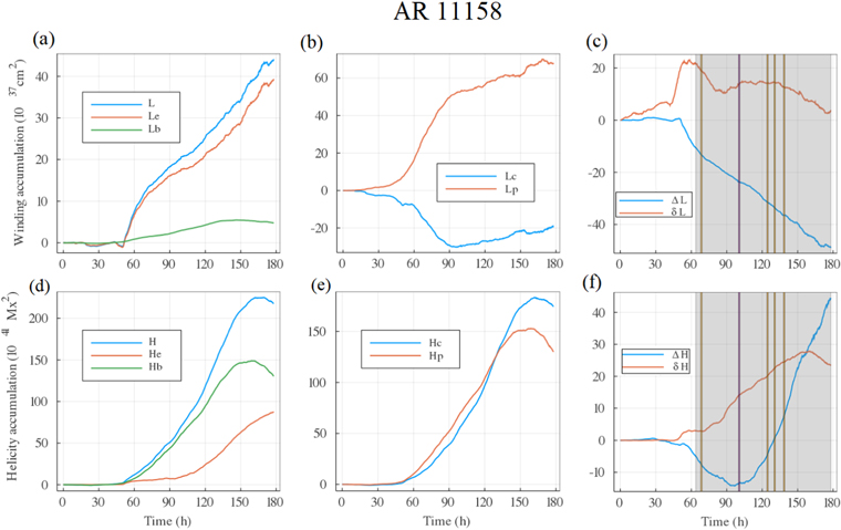
Figure 16. Top: evolution of magnetic winding accumulation in AR 11158, including (a) its emergence/braiding decomposition, (b) its potential/current-carrying decomposition, and (c) the differences between potential and current-carrying windings. The gray region covers the period of the region's flaring activity; the vertical lines are its M- (yellow) and X-class (purple) flares. Bottom: the helicity analysis, including (d) its emergence/braiding decomposition, (e) its potential/current-carrying decomposition, and (f) the differences between potential and current-carrying helicities.
Download figure:
Standard image High-resolution image3.4.4. Evolution of Current/Potential Decompositions
The decomposition of the winding in terms of its potential/current-carrying components shows a stronger input (in absolute value) of potential field compared with the current-carrying part (Figure 16(b)). This is consistent with the overall larger input of potential energy over free magnetic energy observed in Kazachenko et al. (2015). This is an apparent contradiction with the idea we posited earlier that a dominant current-carrying field is necessary for the commencement of flaring activity. A resolution can be found when we compute the local and global difference measures ΔL and δ L. While the global difference ΔL shows a dominance of the potential part (Figure 16(c)), the local difference δ L shows a dominance of the current-carrying component, and, in particular, between 45 and 60 hr there is a significant change in this imbalance, marked by a rapid rise in the imbalance toward current-carrying topology being emerging. The period after this buildup of significant localized positive imbalance in the current-carrying/potential winding difference is marked in gray in Figure 16(c). This coincides with the beginning of flaring activity in this region (indicated by the gray region; M- and X-class flares are marked by yellow and purple vertical lines, respectively). This result backs up the findings from the two previous regions that a significant and sustained buildup of net current-carrying winding is necessary for the commencement of flaring activity. What differs in this case is that the complexity of the region means that this only shows up in the δ L measure, which accounts for local current-carrying/potential balances.
That the localized quantity carries crucial information can be understood by observing the spatial distributions of the winding fluxes  and
and  in Figure 17. We observe, for instance, at time t = 50 hr that there are significant subregions of both positive and negative current-carrying winding input density (Figure 17(c)), while the potential density (Figure 17(a)) is mostly positive. This means that the net current-carrying winding Lc
might be weak owing to cancellations and explains why ΔL is being dominated by the potential contribution. However, locally there are coherent regions with strong positive and negative signs in the current-carrying density
in Figure 17. We observe, for instance, at time t = 50 hr that there are significant subregions of both positive and negative current-carrying winding input density (Figure 17(c)), while the potential density (Figure 17(a)) is mostly positive. This means that the net current-carrying winding Lc
might be weak owing to cancellations and explains why ΔL is being dominated by the potential contribution. However, locally there are coherent regions with strong positive and negative signs in the current-carrying density  that would not be balanced out by potential densities
  in the evaluation of δ
L. A clear example of this imbalance can be seen at t = 100 hr (Figures 17(b) and (d)), in the location centered at pixels x = 400, y = 175, where there is a region of strongly positive current-carrying winding flux
in the evaluation of δ
L. A clear example of this imbalance can be seen at t = 100 hr (Figures 17(b) and (d)), in the location centered at pixels x = 400, y = 175, where there is a region of strongly positive current-carrying winding flux  , but the potential winding flux
  is negligible. There is a similarly obvious patch of negative current-carrying winding flux centered at pixels x = 250, y = 150, which is not balanced by the potential winding flux.

Figure 17. Magnetic winding distributions at two different stages of the evolution of AR 11158, t = 50 hr and t = 100 hr. The potential (top) and current-carrying (bottom) parts are displayed. Green lines represent contour sets for the vertical magnetic field Bz = 1000 G.
Download figure:
Standard image High-resolution imageThe current-carrying and potential helicity inputs are very similar, except near the last 30 hr of the data (when the region has a Carrington longitude greater than 60°r and the data are thus not reliable). The quantity δ H, however, indicates that there is a strong local imbalance in favor of current-carrying helicity flux, which begins at about 50 hr (when there is also a rapid positive input in the δ L time series). After this, it rises steadily until near the end of the data. The spatially averaged ΔH series swings between positive and negative values, indicating, as with the winding decompositions, that there are some regions of strong local imbalance whose information is lost in the spatial average. In short, the measure δ H is confirming the conclusions from the δ L series for regions of significant current-carrying topology.
In Figure 18(a), we present the time series of  . The shaded gray region represents the period of flaring for this region, and the pink region represents the period when the region is beyond a Carrington longitude of 60°r. The vertical purple line represents the X-class flare and the yellow lines the M-class flares, as for Figure 16. We see that about 20 hr before the start of the flaring activity there is a strong and consistent input of topologically significant field dominated by the current-carrying component, which suggests that the rapid increase in δ
L is a precursor for the flaring activity. This is also evidenced by a significant rise in the accumulated δ
L (Figure 17(c)), peaking at 60 hr, just before the flaring. Note that this rise does not lead to any spikes above the 3 standard deviation envelope, as it increases the running mean steadily. It does appear to act as a precursor to the first M-class flare. At about 90 hr we see two positive spikes above the 3 standard deviation envelope about 10 hr before the X-class flare. About 5 hr before the second M-class flare there is again a positive spike, and similarly there are spikes just above the envelope about 2 and 3 hr before the final two, which are indicated by green circles in Figure 18. Therefore, there is some tentative evidence that significant positive deviations from the running mean of the δ
L input rate are early warning signals for flares. We note in all these cases that the accumulated δ
L is always positive and an order of magnitude larger than in the case of AR 11318, so these results are apparently meaningful in the sense that they coincide with a significant imbalance in current-carrying topology having been injected, unlike the spikes seen in AR 12119. The
. The shaded gray region represents the period of flaring for this region, and the pink region represents the period when the region is beyond a Carrington longitude of 60°r. The vertical purple line represents the X-class flare and the yellow lines the M-class flares, as for Figure 16. We see that about 20 hr before the start of the flaring activity there is a strong and consistent input of topologically significant field dominated by the current-carrying component, which suggests that the rapid increase in δ
L is a precursor for the flaring activity. This is also evidenced by a significant rise in the accumulated δ
L (Figure 17(c)), peaking at 60 hr, just before the flaring. Note that this rise does not lead to any spikes above the 3 standard deviation envelope, as it increases the running mean steadily. It does appear to act as a precursor to the first M-class flare. At about 90 hr we see two positive spikes above the 3 standard deviation envelope about 10 hr before the X-class flare. About 5 hr before the second M-class flare there is again a positive spike, and similarly there are spikes just above the envelope about 2 and 3 hr before the final two, which are indicated by green circles in Figure 18. Therefore, there is some tentative evidence that significant positive deviations from the running mean of the δ
L input rate are early warning signals for flares. We note in all these cases that the accumulated δ
L is always positive and an order of magnitude larger than in the case of AR 11318, so these results are apparently meaningful in the sense that they coincide with a significant imbalance in current-carrying topology having been injected, unlike the spikes seen in AR 12119. The  time series, shown in Figure 18(b), has only one spike outside the 3 standard deviation envelope at about 90 hr, at a very similar time to one of the spikes in the
  series. This is about 10 hr before the region's single X-class flare, so the temporal correlation of the spikes might be significant. Also possibly significant is that the running mean of the
  rises to its peak value just before this flare.
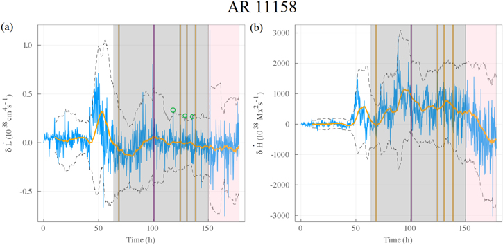
Figure 18. Time series of  and
and  for AR 11158. The format of Figure 7 is used here, with the addition of a gray region indicating the period of flaring.
Download figure:
Standard image High-resolution image3.4.5. Summary and Conclusions from Region
The analysis of this AR provides further evidence that a phase of consistent input of current-carrying-dominated topology is indicative of the onset of flaring activity. The complexity of the region means that a comparison of the localized δ L is required to observe that there is a net imbalance of current-carrying topology, as the complexity of the region means that the net values of Lc are subject to significant cancellations of positive (right-handed) and negative (left-handed) winding. After a large amount of complex current-carrying field is input, as seen in a sustained rapid rise in δ L around t = 50 hr, there should be a large amount of magnetic field energy that can be released. This is evidenced by the commencement of the flaring activity about 10 hr after this rapid increase in input of current-carrying topology. There is also some evidence that δ L has the potential to predict strong individual flaring events from magnetogram data.
3.5. AR 12673
3.5.1. Description of General Activity
In order to verify whether the flaring indicators observed in AR 11158 repeat themselves in other flare-intensive ARs, we analyze AR 12673. This region has been the subject of several other studies owing to its prolific activity, being the most prolific ARs during solar cycle 24 (Sun & Norton 2017).
When AR 12673 appeared on the visible disk, on 2017 September 4, it consisted of a single positive polarity sunspot (see Figure 19(a)). This configuration lasted for 2 days until a bipolar region emerged to the southeast of the original sunspot (see Figure 19(b)). This was followed by the emergence of another bipolar region to the northeast of the original sunspot. The movement of the bipoles then distorted the penumbra of the original sunspot, leading to an elongation of its shape. After that, another pair of bipoles emerged. This sequence of emerging bipole, together with their interaction with the original sunspot, led to a complex magnetic field structure by September 6 (see Figure 19(c)). See Yang et al. (2017) and Sun & Norton (2017) for further details on this region's evolution.
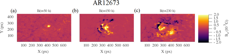
Figure 19. Magnetograms of Bz at three different moments of the evolution of AR 12673.
Download figure:
Standard image High-resolution image3.5.2. Previous Studies of This Region
Possible reasons for such strong eruptivity in this region are also described in Yang et al. (2017; see also Jiang et al. 2019; Liu et al. 2019). This region has also been reported to yield the strongest magnetic fields ever observed in the solar corona (Anfinogentov et al. 2019). AR 12673 appeared on the disk on 2017 August 28, lasting for 13 days. This AR produced 27 M-class flares and four X-class flares, including an X9.3 flare, the largest flare since 2005. AR 12673 was among the ARs analyzed by Deshmukh et al. (2020), where machine-learning techniques were used to study topological changes in the configuration of magnetograms. It was found that an important topological change, related to the connectivity of subgroups of pixels, occurred about 24 hr before the strongest X-class flare.
The analysis of the helicity evolution in AR 12673 based on nonlinear field extrapolations was performed in Moraitis et al. (2019), where it was shown that there was an increase in nonpotential helicity just before major events, after which a relaxation was observed, leading to a more potential-dominated helicity. In addition, Kusano et al. (2020) used an extrapolation-based approach and a flaring metric to identify regions of the constructed field that satisfied certain implied instability criteria for flaring/eruption in the hour before the flares, in particular for the X-class flares of the region. Here we show that similar signatures can be found from the magnetogram data alone.
3.5.3. Evolution of the Basic Topological Quantities
The various topological inputs are shown in Figure 20 and were calculated from SHARP data beginning on 2017 August 28 at 09:00:00 UT. As for all other ARs analyzed, the winding of AR 12673 is dominated by the emergence term (Figure 20(a)). Figure 20(d) shows the evolution of the helicity. We note, by contrast to the results of AR 11158, that the braiding term and the emergence term are of a similar order of magnitude throughout. This is probably because AR 11158's activity is associated with a significant amount of sunspot rotation (see the literature review of that region above), while AR 12673's development is characterized by multiple emergence events throughout its life cycle. The evolutions of winding and helicity (Figures 20(a) and (d)) are consistent in showing a very low activity in the first ∼120 hr, which might explain why the flaring activity took several days to take place.

Figure 20. Evolution of magnetic winding accumulation (top) in AR 12673, including (a) its emergence/braiding decomposition, (b) its potential/current-carrying decomposition, and (c) the differences between potential and current-carrying windings. The helicity analysis (bottom) includes (d) the emergence/braiding decomposition, (e) the potential/current-carrying decomposition, and (f) the differences between potential and current-carrying helicities.
Download figure:
Standard image High-resolution image3.5.4. Evolution of Current/Potential Decompositions
The potential/current-carrying decomposition shows a strong dominance of the current-carrying winding (Figure 20(b)), which is also seen in both δ
L and ΔL (Figure 20(c)), where again the dominance starts to become clearer after about t = 120 hr. It is interesting that, despite this being a magnetically complex region, there is not the significant difference observed between the localized and global differences, which was observed in AR 11158 (Figure 16(c)). Between 120 and 150 hr there is a sustained rapid input in net current-carrying winding (a sharp increase in δ
L) over the potential winding. As was the case in AR 11158, this sharp input is followed shortly by the initiation of flaring activity, as marked by the gray region in Figure 20(c). For clarity here we only plot the X-class flares and the two largest M-class flares. The gray region represents the full time frame over which flaring activity was observed, and the pink region represents a period when the region is classed as unreliable. As with AR 11158, there is a significant increase in the running mean of δ
L, which precedes the flaring by about 30 hr, as seen in Figure 20(c). The end of this rapid input period coincides with the commencement of flaring. We see that the two largest M-class flares are almost coincident with two spikes in the δ
L input rate. It should be said that there are a number of other smaller M-class flares in and around this time period. For this initial study we focus on the X-class flares, where there is a clearer picture. Two days after the flaring activity starts on September 4, this AR produced two consecutive X-class flares: the first one an X2.2 flare, followed by an X9.3 flare. We note that before these two X-class flares there is a sharp jump in the current-carrying/potential imbalance (not so clear in Figure 20(b)). We shall shortly analyze this jump. These features are also clear in the  time series shown in Figure 21(a). The sharp rise in δ
L preceding the first of the X-class flares is seen as a significant peak that somewhat obscures the rest of the plot owing to its scale. For this reason we choose to limit the vertical scale of this plot, but we highlight the fact that the
time series shown in Figure 21(a). The sharp rise in δ
L preceding the first of the X-class flares is seen as a significant peak that somewhat obscures the rest of the plot owing to its scale. For this reason we choose to limit the vertical scale of this plot, but we highlight the fact that the  spike preceding the pair of X-class flares is over 13 × 1038 cm4 s−1, many times larger than any other spike found for this quantity among any of the ARs discussed here. A third X-flare is shown in the plot, an X1.3 flare, which does not seem to correlate with any large peak of
  (or
(or  ). This is in the pink shaded region (corresponding to the AR having a Carrington longitude greater than 60°r), and the data are not considered to be reliable here. As a final note we see, as in AR 11318 and AR 11158, that during the period of flaring the running mean rate of the imbalance in the input of current-carrying helicity (δ
H) is consistently positive. We also note that there are spikes above the 3 standard deviation envelope prior to the first two large X-class flares, one about 10 hr prior.
). This is in the pink shaded region (corresponding to the AR having a Carrington longitude greater than 60°r), and the data are not considered to be reliable here. As a final note we see, as in AR 11318 and AR 11158, that during the period of flaring the running mean rate of the imbalance in the input of current-carrying helicity (δ
H) is consistently positive. We also note that there are spikes above the 3 standard deviation envelope prior to the first two large X-class flares, one about 10 hr prior.

Figure 21.
 and
and  time series for AR 12673. X-class flares are highlighted with purple vertical lines, while M-class flares equal to or above M.5 intensity are highlighted in yellow. The flaring activity begins with the gray background, while the pink background indicates the period when the AR is situated near the limb (beyond a Carrington longitude of 60°).
Download figure:
Standard image High-resolution image3.5.5. A Submergence Event
Given that AR 19673 produced the strongest flare in 12 yr (X.9), it is interesting to investigate the topological changes in the magnetogram data, measured by the evolution of the magnetic winding, in the time interval around this event. Figures 22(a)–(c) show the configuration of the magnetic winding distribution before this event (Figure 22(a)), at the exact moment of the extreme peak in the input of winding that preceded the consecutive X2.2 and X.9 flares by about 3 hr (Figure 22(b)), and after this event (Figure 22(c)). We observe in Figure 22(a) that, at time t = 210 hr, the magnetic field configuration is complex (green curves represent ∣Bz ∣ = 103 G), with regions of strong winding surrounding the regions with intense magnetic field. At the time of the peak in the input of new magnetic field topology t = 212 hr 36 minutes (Figure 22(b)), we observe intense winding density located around a region centered at approximately x = 270, y = 300 (note that the scale at this time is around 20 times larger than in the other two figures). On closer inspection, we did not find a significant change in the vertical magnetic flux (Bz ) configuration from panels (a)–(c). After both X-class events, the configuration of the winding density shows again a strong input of topologically significant field only in the vicinity of the regions with strong magnetic fields. Figure 22 (middle) shows the vertical velocity distribution vz . There is a region of strong downflow that is intensified at t = 212 hr 36 minutes, with speeds close to 1000 m s−1. A comparison with the above row shows that this is spatially coincident with the location of strong winding flux. This suggests that small subregions with strong vertical velocity (in this case negative) can be the source of spikes in the magnetic winding. Although the magnetic winding is an intrinsically nonlocal quantity, it can be associated with a local quantity, the emergence velocity ve = −vz ∣ B h ∣/Bz , which is presented in the bottom row of Figure 22. We see that the strong winding is associated with a strong localized region of ve (again roughly centered at x = 270, y = 300). In Figure 23, the distributions of magnetic winding, vertical velocity, and emergence velocity are zoomed in around the region of strong winding at t = 212 hr 36 minutes, showing that there is a change in the sign of ve . Since ∣ B ∥∣ > 0 and vz < 0 in that region, an inversion in ve is associated with a sharp inversion of Bz , indicating a polarity inversion line. The inversion of Bz in such a small region associated with the downflow might be related to reconnection events, which are known to play an important role in solar flares (Shibata 1998). This strong and localized winding signature, several hours before the large flares, could be an example of tether-cutting reconnection in the low atmosphere (Moore et al. 2001). Indeed, Kusano et al. (2020) also identify this localized region on the PIL, by another topological approach, as the location of the first of the large X-class flares.
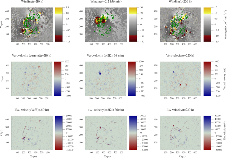
Figure 22. Evolution of the magnetic winding flux (top), vertical plasma velocity (middle), and emergence velocity (bottom) before and after the X.9 flare event produced by AR 12673. Note that the scale in panel (b) is 20 times larger than that of panels (a) and (c), reflecting the intensity of the winding input at that particular time.
Download figure:
Standard image High-resolution image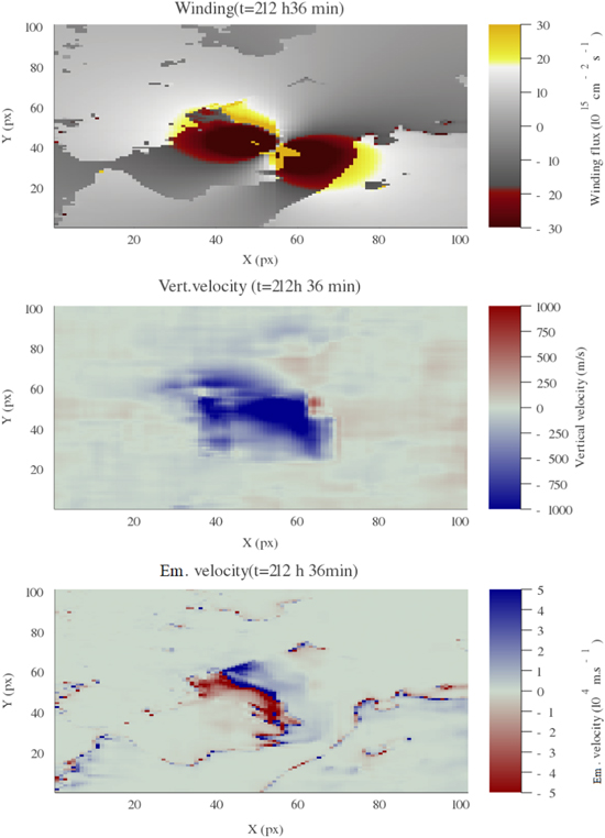
Figure 23. The magnetic winding flux (top), vertical plasma velocity (middle), and emergence velocity (bottom), zoomed in around the region of intense winding during the most intense peak of winding input at t = 212 hr, 36 minutes.
Download figure:
Standard image High-resolution imageThis small part of the AR dominates the winding, due to a downflow associated with a polarity inversion. It is, therefore, interesting to compare how the accumulated flux of winding differs between different parts of the AR. In Figure 24 we split AR 12673 into 16 (4 × 4) rectangular subregions of the same size. As expected, the parts of the AR with strongest winding input correspond to parts near the strong winding spot shown in Figure 23. Rectangles 2–2 and 3–2 show an accumulated winding that is ∼4 × larger than the accumulated winding on the border of the AR. There is some evidence, then, that this significant loss of current-carrying topology sets off an evolution of the field that leads to the eventual flare. This is consistent with the sharp spike in  seen prior to the flare event in AR 11318 (Figure 7(a)).

Figure 24. Magnetic winding accumulation in AR 12673 divided into 16 (4 × 4) equal rectangular subregions.
Download figure:
Standard image High-resolution image3.5.6. Summary and Conclusions from Region
The magnetic winding evolution associated with AR 12673 is clearly dominated by its current-carrying component, as seen in Figure 20. As in the case of AR 11158, the start of the flaring activity is preceded about 30 hr by a strong and consistent input of current-carrying-dominated magnetic winding, as seen in Figure 21. This input is most sharply observed in the localized measurement δ
L. The two consecutive X-class flares, including the strongest X.9 flare, are preceded by a strong spike in  roughly 5 hr prior to the event, suggesting that this large perturbation, traced to the disappearance of a localized bipole of strongly current-carrying magnetic field, led to a dramatic restructuring of the magnetic field that then resulted in the flares. It is particularly interesting that a clear precursor to these flares is observed at the photosphere. Overall, the results from this region reinforce those of the previous regions, i.e., that the quantities δ
L and δ
H, used in conjunction, have significant predictive potential for flaring events.
roughly 5 hr prior to the event, suggesting that this large perturbation, traced to the disappearance of a localized bipole of strongly current-carrying magnetic field, led to a dramatic restructuring of the magnetic field that then resulted in the flares. It is particularly interesting that a clear precursor to these flares is observed at the photosphere. Overall, the results from this region reinforce those of the previous regions, i.e., that the quantities δ
L and δ
H, used in conjunction, have significant predictive potential for flaring events.
4. General Summary and Conclusions
In this work, we have analyzed magnetic winding and magnetic helicity fluxes for five ARs. This was with with a view to discovering a (potentially) reliable metric that can help forecast the likelihood of flaring, and, in particular, one that can be calculated without the need for three-dimensional extrapolations of the magnetic field. The first three regions (AR 11318, AR 12119, and AR 12285) are relatively simple bipolar regions with minimal intrinsic flaring activity (though the first two are related, in different ways, to CMEs). The final two (AR 11158 and AR 12673) are much more complex regions with significant flaring activity. All calculations are based on magnetogram data only, and the magnetic field is decomposed to potential and current-carrying parts. This decomposition of the magnetic field is used to create further decompositions of the magnetic helicity and winding fluxes. We analyze the behavior of these flux decompositions in relation to the onset of flaring within the AR. One quantity in particular, δ
L, which is the total sum of a pixel-wise (absolute) comparison of current-carrying and potential winding flux distributions, has been shown to give a consistent picture of when flaring may occur. When δ
L > 0, this indicates a local dominance of the current-carrying contribution compared to the potential contribution. All flaring regions studied exhibit a significant positive increase in δ
L in the hours before the onset of flaring. By contrast, the regions AR 12119 and AR 12285, which had no internal flaring, did not have a consistent buildup of positive δ
L. For AR 12673, we have shown that a rapid increase in δ
L, before the onset of an X-class flare, can be traced to a particular area of the AR where there is a localized downflow and subsequent disappearance of a coherent magnetic structure with an MPIL associated with a strong localized winding signature. Such behavior is highly suggestive of a dramatic localized change in field topology, a change that then evolves to produce a strong flare. The fact that this signature is detected from magnetogram data indicates that the emergence and submergence of topologically complex magnetic field are important for the development of flares. A critical point about this particular example is that the region that caused the spike correlates spatially and temporally with a sigmoidal structure obtained in nonlinear force-free extrapolations performed in Kusano et al. (2020). In addition, we identified a number of similar events with sharp changes in the quantity rate  , which preceded significant flaring events by a similar time period (about 7 hr) on both AR 12673 and AR 11158. These sharp positive changes (spikes) are defined to occur when a spike value is greater than 3 standard deviations from a 10 hr running mean. We also found that spikes in regions with negative δ
L did not indicate flaring activity, so the combination of the rate
, which preceded significant flaring events by a similar time period (about 7 hr) on both AR 12673 and AR 11158. These sharp positive changes (spikes) are defined to occur when a spike value is greater than 3 standard deviations from a 10 hr running mean. We also found that spikes in regions with negative δ
L did not indicate flaring activity, so the combination of the rate  and the accumulated value δ
L indicates a potential predictive capability.
and the accumulated value δ
L indicates a potential predictive capability.
Although the spotlight in this work has fallen on δ L owing to its efficacy in signaling the onset of flares, this does not mean that decompositions and metrics of helicity, such as δ H, should be disregarded. When applying the techniques described here to a larger number of ARs, there may be winding time series with spikes that are difficult to interpret or do not correspond to dynamically significant magnetic field. In such a scenario, helicity could help to distinguish whether or not a spike in the winding time series is significant.
In summary, the winding and helicity flux quantities that we have calculated give important information about AR evolution, with δ L, in particular, providing an early warning signature for the onset of flaring activity. In future work, we will extend our analysis to a much larger set of ARs to evaluate the consistency of this measure over a wider variety of ARs and also whether it can be incorporated into other predictive methodologies.
D.M., C.P. and B.R. welcome support from the US Air Force Office for Scientific Research (AFOSR): FA8655-20-1-7032.
Appendix: Testing Different Parameters in the Winding Calculations
The calculations of the magnetic winding performed here depend on two parameters: (1) the cutoff of the magnetic field strength (BC ), and (2) the smoothing window size (VS) in the DAVE4VM velocity inversion technique (Schuck 2008). Here we present a sensitivity analysis (see Figure 25) based on AR 11318 by calculating the evolution of the quantities δ L and ΔL using parameters BC = 50, 100, and 200 G and VS = 12 and 20 pixels. The calculations for δ L show qualitatively similar results for parameters (BC = 50 G, VS = 12 pixels), (BC = 50 G, VS = 20 pixels), (BC = 100 G, VS = 12 pixels), (BC = 100 G, VS = 20 pixels). The peak values of δ L tend to decrease with the size of the smoothing window for the same magnetic field cutoff, since with large smoothing windows fewer small-scale magnetic structures are resolved in the inversion. This difference, however, is smaller than the decrease due to the magnetic field cutoff. For all parameter sets with BC < 200 G the quantity ΔL shows the same rise-then-fall shape. What is interesting is that the peak is delayed for smaller smoothing windows. Again, this is suggestive that smaller-scale field is affecting the velocity and hence winding input. It is also noticeable that with the 12-pixel smoothing, the value always remains positive, and by the end of the time series the difference is quite significant (for a given fixed cutoff BC ).

Figure 25. Magnetic winding calculations for AR 11318 calculated with different parameters BC = 50, 100, and 200 G and VS = 12 and 20 pixels.
Download figure:
Standard image High-resolution image
In summary, the quantity δ L is far more stable to variations in the choice of velocity smoothing than ΔL. In addition, there is a significant loss of current-carrying topology measured if the magnetic field cutoff is large, in particular between 50 and 200 G.