


Abstract
The "equal-contrast technique" (ECT) methodology, developed by Singh et al. to generate uniform long time series of Ca-K images obtained during the 20th century from the Kodaikanal Observatory (KO), improved the correlation between the plage area and sunspot parameters. The same methodology can also be used on other observatory data taken with different instruments. We can combine such ECT-corrected images to reduce the gaps in the observations and make a long uniform data set to study short- and long-term variations. We apply this procedure to Mount Wilson Observatory (MWO) historical Ca-K data and recent Ca-K filtergrams obtained using narrowband filters at KO and the Mauna Loa Solar Observatory (MLSO). To determine the success of this method, the results of the analysis of the ECT images obtained from KO, MWO, and MLSO are compared. A comparison of the plage and active areas derived from KO and MWO images before and after the ECT procedure indicates an improvement in the correlation coefficients (CCs) between all the data sets after the ECT application. The CC for the combined monthly mean Ca-K plage area derived from the KO, MWO, and Precision Solar Photometric Telescope (at the MLSO) data with sunspot numbers is 0.96 for the period 1905–2015. The paper demonstrates that the time series of Ca-K data obtained from different instruments after applying the ECT procedure becomes uniform in contrast. The combined time series of KO and MWO spectroheliograms has 12 hr intervals compared to the ≈24 hr gap for a time series from a single observatory.
Export citation and abstract BibTeX RIS

Original content from this work may be used under the terms of the Creative Commons Attribution 4.0 licence. Any further distribution of this work must maintain attribution to the author(s) and the title of the work, journal citation and DOI.
1. Introduction
Long-term information on the strong and weak magnetic fields on the Sun is very important to understand the dynamo processes. The complex dynamo process thought to operate at a layer just below the convection zone, known as the tachocline (Gilman 2000; Weiss & Tobias 2000), causes visible variations on the solar surface. This process leads to solar cycle activity, such as 11 yr periods, which influences the space weather and climate (Foukal et al. 2009; Solanki et al. 2013). The study of the systematic variation of the activity on the solar surface helps us to understand the evolution of two (poloidal and toroidal) components of magnetic fields (Choudhuri et al. 1995). Using line-of-sight magnetograms and Ca-K spectroheliograms, several authors showed a strong correlation between them (Babcock & Babcock 1955; Leighton 1959; Stepanov 1960; Leighton 1964). The study of Ca-K bright points and small-scale magnetic fields by Sivaraman & Livingston (1982) indicated a correlation between the two. The Ca-K plage and networks can be a proxy to study the variations in magnetic fields as there is a strong correlation between Ca-K intensity and magnetic fields (Skumanich et al. 1975; Schrijver et al. 1989; Ortiz & Rast 2005).
Hale (1890) and Deslandres (1891) independently invented the spectroheliograph (the principles of the spectroheliograph were first described by Janssen 1868; see also Hale 1929). Observations in the Ca-K line have been acquired at various observatories since the beginning of the 20th century first, using spectroheliographs and, later, narrowband filters (Bappu 1967; Bertello et al. 2016; Singh et al. 2018; Bertello et al. 2020). The historical data recorded on photographic plates and films at Mount Wilson Observatory (MWO) were digitized by Foukal (1996) for the first time in 512 × 512 format with an 8 bit readout signal. At most of the observatories before the use of digital detectors, a couple of images per day were obtained using photographic plates and films. Tlatov et al. (2009) digitized Ca-K spectroheliograms from Kodaikanal Observatory (KO) for the period 1907–1999 using a commercial flatbed 8 bit scanner. Several authors extensively used these digitized data to investigate the variation in the chromosphere with time, correlation with other solar activity indices, and climatic variation on Earth (Ermolli et al. 2009; Foukal et al. 2009; Bertello et al. 2010). The Ca-K spectroheliograms obtained at KO for the period 1905–2007 were digitized with a pixel resolution of 0 86 and 16 bit readout (Priyal et al. 2014, 2017).
Tlatov et al. (2009) analyzed the digitized Ca-K images of KO and MWO and compared the derived plage areas for each solar cycle for the period 1915–1985. They found that the identified plage area for the MWO data is larger for each solar cycle by about 30% compared to KO images. Further, they reported that the difference was significant during cycle number 19. Ermolli et al. (2009) analyzed the images from the KO, MWO, and Arcetri (Ar) and found that the quality of the data varies with time in all three series. They interpreted these variations as changes in instruments, aging of the optics used, and modifications of the observing programs. They found that yearly median values of the plage area for the three analyzed series differ.
Bertello et al. (2010) determined the Ca-K index by using the Ca-K images from MWO and found that the yearly average data agree with the Ca-K plage index measured from the KO and National Solar Observatory (NSO) at Sacramento Peak (SP). They extended the Ca-K index series by determining the relationship between Ca-K and the magnetic field strength (MPSI) measured at MWO and used the MPSI data as a proxy for the Ca-K index. Chatzistergos et al. (2019) used data from eight observatories, namely the Arcetri, KO, McMath-Hulbert, Meudon, Mitaka, MWO, Schauinsland, and Wendelstein observatories, as well as one archive of filtergrams from the Precision Solar Photometric Telescope (PSPT)/Rome to construct a composite series of plage areas as a function of time. They found that comparing the two longest series of spectroheliograms indicates that the percentage of plage area determined from MWO data is more than the KO images.
Most authors could study the variations in the fractional plage area but not the small-scale networks because of nonuniformities in the data due to a number of reasons (Foukal 1996; Lefebvre et al. 2005; Tlatov et al. 2009; Sheeley et al. 2011; Priyal et al. 2014; Chatzistergos et al. 2019). Further, most of the analyses done indicate that each data set yields different results depending upon the instrument's specification and digitization of the data. We note that the quality of the images also varies with time at the observatory due to changes in the instrument and emulsion. It is, therefore, necessary to develop a uniform series of images from all observatories to study the short- and long-term variations. Using a different methodology, Bertello et al. (2020) rescaled the intensity of about 16,000 MWO images such that the FWHM of the intensity distribution of each image was 0.08. They showed an excellent correlation between the sunspots and the Ca-K index and investigated the chromospheric differential rotation.
Large-scale magnetic field studies of the Sun are very important because they provide a clue to the underlying dynamo processes that produce the magnetic fields and also study their effect on Earth's climate and space weather. To study the long-term variations in solar magnetic fields, it is essential to have a long-term solar data set. Though it is possible to get the long data set from one observatory, there are data gaps due to weather conditions at the site, absence of observers, working conditions of the telescope and associated instruments, and so on. To fill in those data gaps, one can use data from other observatories. The combined data from different observatories will be nonuniform due to different spatial resolutions and passbands of the spectroheliograph or the filter used. The narrow bandpass of the Ca-K filter/exit slit of the spectrograph increases the contrast of the image. The contrast of the image affects the detection of features such as plage and networks in terms of their area and intensity. Recently, several studies have attempted to develop homogenized data sets of Ca-K line images using historical observations from various observatories (Pevtsov et al. 2016; Chatzistergos et al. 2019; Bertello et al. 2020) with partial success. Singh et al. (2021) developed a methodology called the equal-contrast technique (ECT) to make the image contrast uniform over a long time series of Ca-K images of the Sun from the KO data. The application of this methodology on the long time series of KO images showed uniform contrast over century-long time-series Ca-K data (Singh et al. 2021). To determine the uniformity of the contrast of the data after ECT application, it is good to compare the derived Ca-K parameters such as the plage and active area extracted from all the Ca-K data sets on short and long timescales. "Active area" is defined as the region of the Sun whose intensity is greater than that of the quiet chromospheres. Thus, it includes the plage and small bright regions, which are fragments of the plage areas (Worden et al. 1998). The intensity threshold values of these will be discussed in Section 3.
In the present paper, we examine how suitable the ECT is for the creation of a single, homogenized, long time series of Ca-K images obtained using instruments with significantly different characteristics (bandpass, aperture, etc.). We have analyzed Ca-K images of the Sun obtained with instruments at MWO, Kodaikanal Observatory (KO), and the PSPT and applied the ECT methodology to them. This paper provides the details of the analysis of the KO, MWO, and PSPT data sets after applying the ECT methodology to those data series. In Section 2, we describe the details of the data, their spatial resolution, the passband of the exit slit or the filter, the FWHM of the intensity distribution before and after the ECT methodology, etc. In Section 3, we compare the area occupied by the observed Ca-K features from each of these data set with the sunspot number and area before and after applying the ECT methodology. The paper ends with a summary of the obtained results and discussions.
2. Data and Analysis
We have analyzed five different types of data obtained from three observatories, namely KO, MWO, and PSPT operated at the Mauna Loa Solar Observatory (MLSO) in Hawaii. The types of instruments used in each observatory are listed in Table 1. We have already reported the results of the KO spectroheliograms after applying the ECT methodology in Singh et al. (2021). We identify this time series as "data set-1". The ECT methodology is to make the images of uniform contrast. If the FWHM of the intensity distribution is larger than the chosen interval of 0.10–0.11, it indicates the image has high contrast. Then, the intensity values of the image are rescaled such that the FWHM values lie between 0.10 and 0.11. Similarly, the FWHM of the intensity distribution being less than the chosen interval indicates a low-contrast image. The intensity distribution is then rescaled so that the FWHM also lies between 0.10 and 0.11. Thus, the FWHM of the intensity distribution of all images between 0.10 and 0.11 implies a uniform contrast of all time series. At KO, the Ca-K filtergrams are taken with the 2.5 Å passband filter centered at 3933.7 Å using a 1024 × 1024 CCD camera during 1998–2007 with a 15 cm telescope of 225 cm focus (data set-2). The Ca-K filtergrams are obtained with the same narrowband filter and 2048 × 2048 CCD camera mounted on the 15 cm telescope of 225 cm focal length during 2008–2013 (Singh & Ravindra 2012; Singh et al. 2012, data set-3).
Table 1. Name of the Observatory, Data Type, Period of Observations, Total Number of Images Analyzed, Number of Days of Data Analyzed, Bandwidth of Observations, and Pixel Resolution of the Digitized or Observed Data
| Observatory | Data Type | Period | Total No. | No. of Days | Bandwidth | Pixel Resolution |
|---|---|---|---|---|---|---|
| of Images | of Data Analyzed | (Å) | (arcsec) | |||
| KO (DS-1) | Sp | 1905–2007 | 34453 | 16981 | 0.5 | 0.86 |
| KO (DS-2) | Fi | 1997–2007 | 10065 | 2710 | 2.5 | 2.23 |
| KO (DS-3) | Fi | 2008–2013 | 11781 | 1163 | 2.5 | 1.21 |
| MWO (DS-4) | Sp | 1915–1985 | 36050 | 10996 | 0.35 | 0.95 |
| PSPT/MLSO (DS-5) | Fi | 1998–2015 | 7309 | 2489 | 2.73/1.0 | 1.03 |
Notes. Sp and Fi stand for spectroheliograms and filtergrams, respectively. "DS" stands for data set.
Download table as: ASCIITypeset image
We have downloaded the digitized Ca-K 2600 × 2600 high-resolution spectroheliograms from MWO with a pixel resolution of 095 (data set-4). We downloaded a couple of Ca-K images per day from the MWO website. The downloaded images are already calibrated for the density-to-intensity conversion but have not been flat-fielded. Several Ca-K filtergrams were obtained per day with a PSPT telescope at MLSO in Hawaii (data set-5). We randomly selected three images per day for our analysis. These images were already corrected for the limb-darkening effect as indicated in the image header (Rast et al. 2008). The details of the data are listed in Table 1.
2.1. FWHM of the Intensity Distribution
All recent and historical images taken or digitized using a CCD camera are in 16 bit readout format. Images from MWO (spectroheliograms), PSPT, and KO (filtergrams) were corrected for large-scale intensity variations due to instrumental artifacts or sky transparency using the procedure adapted by Priyal et al. (2017, 2019). This was done in two stages: first, using the polynomial fit to quiet-chromosphere pixels in a row and then normalizing the intensity values of the original image by its polynomial fit. This was repeated for pixels in each row of the image. The same procedure was applied to the pixels in columns. Second, the resultant image was segmented into eight rings of equal areas, and each ring was divided into 12 segments of 30° each. After that, 35% of the pixels whose intensity values are larger in each segment were replaced by the average value of the remaining pixels. The resulting image was smoothed using an 8 × 8 pixels box. This generated the background image of the chromosphere. The image obtained after the first stage of the operation was divided by the background image and then normalized using a Gaussian fit to the intensity distribution of the image. More details of the analysis can be seen in the papers of Priyal et al. (2014, 2017, 2019).
The contrast of each image was then adjusted using the ECT methodology to constrain the FWHM of the intensity distribution between 0.10 and 0.11 as defined by Singh et al. (2021). In Figure 1, we show the histogram of the FWHM values of an image before ECT application for four data sets. In Figure 1, the upper-left and -right panels show the histogram of the FWHM values for the KO and MWO spectroheliograms, respectively. The range of FWHM values is 0.02–0.32 for KO spectroheliograms and 0.01–0.40 for the MWO data, which implies that the contrast of the images varied more for the MWO data than for the KO data. The two lower panels of the figure show the histogram of the FWHM for the KO and PSPT filtergrams. The histograms of the filtergrams shown in the bottom row of Figure 1 indicate that the FWHM values range between 0.02–0.07 and 0.03–0.08 for the KO and PSPT/MLSO data, respectively. The FWHM values of the filtergrams imply that the contrast of the filtergrams is less than that of spectroheliograms. Therefore, the contrast of the filtergrams was increased to that of the spectroheliograms by increasing the FWHM using the ECT procedure.

Figure 1. Top-left and -right panels of the figure show the histograms of the FWHM values of the intensity distribution before the ECT application for the KO and MWO spectroheliograms, respectively. Bottom-left and -right panels show the histograms of the FWHM values for the KO and PSPT filtergrams.
Download figure:
Standard image High-resolution imageFigure 2 (top) shows the FWHM values of all the images obtained between 1905 and 2015 before applying the ECT methodology. The plot shows both long- and short-term variations in the contrast of the images. Large variations in the FWHM of the intensity distribution of spectroheliograms are because of uncertainty in visually centering the Ca-K line on the exit slit of the spectrograph. The FWHM of the intensity distribution for PSPT filtergrams remains the same during the observing period of 1998–2015 with minor variations due to sky conditions. But, in the case of the KO filtergrams, the FWHM starts decreasing after 2009 due to the degradation of the narrowband Ca-K filter. The bottom panel of Figure 2 shows the FWHM values of the spectroheliograms and filtergrams as a function of time after applying the ECT procedure. In the plot, it is clear that the FWHM values of all the images lie between 0.1 and 0.11.

Figure 2. The upper panel shows the FWHM value of the normalized intensity distribution for all data (spectroheliograms and filtergrams) before the application of the ECT procedure. Different colors represent data obtained from different instruments as indicated in the figure. The bottom panel shows the same for all the images after the application of the ECT procedure. The y-axis scale is different from that in the top panel.
Download figure:
Standard image High-resolution imageThe top two panels of Figure 3 show a sample of digitized MWO images and their intensity distributions. The middle two panels show the image and its intensity distribution after the limb-darkening and instrumental vignetting corrections but before the ECT application. The intensity distribution of this image shows a relatively broad FWHM, which is a signature of high-contrast images. The bottom two panels show the image and intensity distribution after the ECT application. The plot clearly shows that the width of the distribution is reduced and the height is increased after the ECT. The FWHM of the intensity distribution is found to be between 0.1 and 0.11 after the ECT. The intensity distribution for all the Ca-K filtergrams obtained at KO and PSPT becomes broad after the application of the ECT procedure.

Figure 3. The top two panels of the figure show the Ca-K image taken on 1958 May 5 at MWO and its intensity distribution. The middle two panels indicate the flattened image using the code developed for KO data and intensity distribution. The bottom two panels show the image and its intensity distribution after using the ECT methodology developed for KO data.
Download figure:
Standard image High-resolution image3. Results
After applying the ECT procedure to the time series of KO, MWO, and PSPT Ca-K images, we obtained the equal-contrast image data set. In order to examine how well the ECT methodology worked on the KO, MWO, and PSPT data sets, we analyzed the extracted features such as plages and active areas (this includes plages and small bright regions whose intensity is more than that of the quiet chromosphere). The plages are identified as regions with intensity values >1.30 and active areas with intensity >1.20. These two parameters were chosen for comparison because earlier works used the same parameters (Priyal et al. 2019; Singh et al. 2021). In Section 3.1, we compare the percentage of plage and active areas derived from the KO and MWO data before and after the ECT application to show that ECT increases the uniformity in both data sets. In Section 3.2, we compare the derived parameters after the ECT application with the sunspot number and areas to confirm that the variation in these agrees with that in the sunspot data.
3.1. Comparison between the KO and MWO Data Sets
We first compare the derived plage and active areas for the KO and MWO data before and after the ECT application to see the effect of the ECT procedure. The left panel of Figure 4 in the top row shows the scatter plot of the plage area between KO and MWO derived before the application of ECT and the right panel after the ECT. It may be noted that the only difference between the two data sets is that image contrast has been normalized by rescaling the intensity distribution of the images using the ECT methodology. The values of the correlation coefficients (CCs) are 0.46 and 0.72 before and after ECT application, respectively. The slopes and intercepts of the linear fit are 1.2 (0.8) and −1.0 (0.1) for the data before (after) the ECT procedure. The intercept value close to zero suggests that the differences between the KO and MWO time series have reduced after the ECT methodology was used. The values of the CC, slope, and intercept and the amount of scatter indicate that there is a large improvement and agreement in the derived plage areas for both data sets after ECT application. This implies that the uniformity of the contrast of the data has increased. The two panels in the bottom row of Figure 4 show the scatter plot of the active area derived from KO and MWO data before and after ECT application. As in the case of plage areas, the plots indicate the value of the CC has increased for active areas after applying the ECT.

Figure 4. The upper-left and -right panels of the figure show the scatter plot between the MWO and KO plage areas before and after the application of ECT, respectively. The two panels in the bottom row show the scatter plot between the MWO and KO active areas before and after ECT application. The values of the correlation coefficient, slope, and intercept of the linear fit are shown in the respective panels.
Download figure:
Standard image High-resolution imageFigure 5(a) shows the derived percentage of the plage area for the KO (black dots) and the MWO data (red dots) for the period 1915–1985 before ECT application. In the plot, the KO plage area varies between 0% and 20%, and the MWO data vary between 0% and 25%. After ECT application, the KO and MWO plage area vary in the range 0%–8% and 0%–10%, respectively (panel (b)). Panel (b) indicates that the derived percentage of plage areas from KO and MWO data agree with each other for the period 1915–1976 but differ for the period 1977–1983. The difference is due to the poor quality of KO images during 1977–83 (Singh et al. 1988). In order to find out how well the two times series match, we plotted the residuals of the difference of the monthly averaged plage area and show them in panel (c) for the time series before ECT application and in panel (d) for after ECT application, respectively. The 13 month running mean values (red dotted curve) of the residuals are overplotted in both panels for comparison. The mean and standard deviation (SD) of the residuals are 0.91 and 3.3 for the panel (c) time series and 0.31 and 0.72 for the panel (d) time series. The comparison of the residual mean and SD of both panels suggest that the differences between the derived values reduced after ECT application.
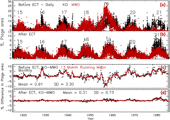
Figure 5. Panel (a) in the figure shows the derived percentage of the daily plage area from the KO (black dots) and MWO (red dots) images before the application of ECT. Panel (b) shows the same after the application of ECT. Panel (c) shows, in black dots, the residuals (KO – MWO) of the derived percentage of plage area for the images before ECT application on a monthly averaged basis. The 13 month running mean values are indicated by red dots. Panel (d) shows the residuals after ECT application. The solar cycle numbers are also marked in the figure.
Download figure:
Standard image High-resolution imageFigures 6(a) and (b) show the percentage of daily active area for the KO (black dots) and MWO (red dots) data before and after ECT application, respectively. Panels ((c) and (d)) of the same figure show the residuals of the differences between the KO- and MWO-derived active area time series, before and after ECT application, respectively. The red curve is the 13 month running mean of the difference. The mean and SD values are computed for the residual time series and are shown in their respective panels. The comparison of these mean and SD values indicates that the ECT methodology reduced the differences between the two data sets.
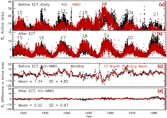
Figure 6. Same as that of Figure 5 but for a percentage of active area.
Download figure:
Standard image High-resolution image3.2. Correlation between Sunspot Number, Area, and Ca-K Plage Area
The sunspot data are the longest and most reliable time series as these have been generated by combining a large amount of observations from several observatories. We, therefore, compare the Ca-K parameters derived after ECT application with the sunspot data to confirm the effectiveness of the ECT methodology. The upper-left and -right panels of Figure 7 show the scatter plot of the Ca-K plage areas from the KO and MWO spectroheliogram daily data versus sunspot numbers (WDC-SILSO, Royal Observatory of Belgium, Brussels, https://wwwbis.sidc.be/silso/). The two panels in the second row show the scatter plots of Ca-K plage areas versus sunspot numbers for KO and PSPT filtergram data. A linear least-squares fit to each data set is also shown in the plots. There is a very good correlation between the plage areas and the sunspot numbers. The values of the CC, slope of the linear regression, and intercept, along with their SD values, are written in the respective panels. The values of the slope of the linear fit representing the sunspot number/plage area are the same for the KO and MWO data, within statistical uncertainties. The values of the CCs between the Ca-K percentage of the plage area and sunspot number are higher compared to those between Ca-K and sunspot area.

Figure 7. The upper-left and -right panels of the figure show the scatter plot between the plage area and sunspot number for the KO and MWO spectroheliograms on a daily basis, respectively. The left and right panels in the second row show the same for KO and PSPT filtergrams on a daily basis, respectively. The period of observation for each set of data is indicated in the plot. The linear fit to the data is also shown by the red line. The values of the correlation coefficient, slope, and intercept, along with their standard deviations (SD), are written in each panel. Similarly, the panels in the third and fourth rows show these scatter plots for sunspot areas instead of numbers.
Download figure:
Standard image High-resolution imageThe panels in the third and fourth rows of Figure 7 show the scatter plots of the plage area derived from KO spectroheliograms, MWO spectroheliograms, KO filtergrams, and PSPT filtergrams versus the sunspot areas obtained from the Greenwich observatory (https://solarscience.msfc.nasa.gov/greenwch.shtml). The values of the CC, slope, and intercept, along with their SD, are indicated in the respective figures. After computing the value of the CC, the confidence level is computed using a t-test. The confidence level is more than 95% for the computed correlation value. This indicates that there is a good correlation between the derived plage area and sunspot parameters. Though the Ca-K plage area derived from KO, MWO, and PSPT shows a good correlation with the sunspot numbers and area, there is a difference in the slope of the filtergrams compared to that of the spectroheliograms. Similarly, the four panels of Figure 8 show the scatter plot of the derived percentage of the Ca-K active area versus sunspot numbers after ECT application for all data sets on a daily basis. The values of the CCs and slope of the linear regression, along with their SD values, are written in the respective panels. The values of the CCs between the percentage of Ca-K active area and the sunspot numbers are in the range of 0.82–0.89 for all data sets, with confidence level >95%. The small difference could be due to statistical studies of large databases and some uncertainty in observations. The ECT does not make the data perfect but improves the homogeneity.
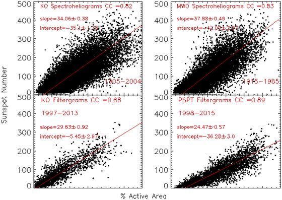
Figure 8. The two panels in the upper row of the figure show the scatter plot of the percentage of active area vs. sunspot numbers for the KO and MWO spectroheliograms. The two panels in the bottom row show the same for the KO and PSPT filtergrams. The value of the correlation coefficient, linear fit, slope of the fit, and intercept are shown in the respective panels.
Download figure:
Standard image High-resolution image3.3. Solar Cycle Variation of the Percentage of Plage Areas
In order to examine how well the KO, MWO, and PSPT data sets match each other after applying the ECT methodology, we have plotted the percentage of daily plage area derived from the spectroheliograms for the observing period 1905–2007 in Figure 9. The black and red dots show the plage area for the KO and MWO spectroheliograms, respectively. The plage area for the PSPT and KO filtergrams are shown in light-green, light-blue (223 pixel−1), and blue dots (121 pixel−1), respectively, for the period 1997–2015. The yearly averaged plage areas are shown in the same plot in their respective colors for easy comparison. The yearly average of the percentage of plage area for the KO spectroheliograms and filtergrams agree with each other even though the yearly data sample was less during the 23rd cycle.
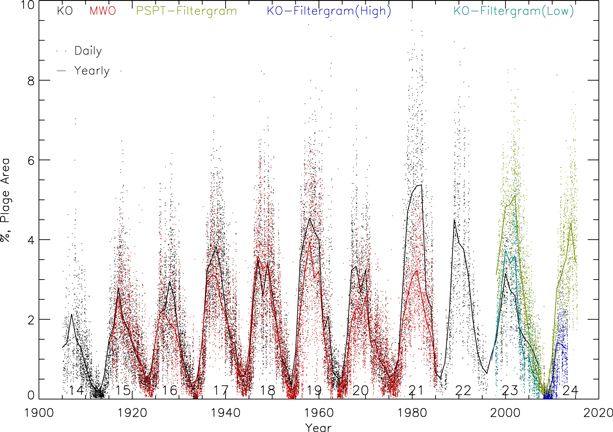
Figure 9. The percentage of area covered by the plages on the Sun is shown by dots for the KO, MWO, and PSPT spectroheliograms and filtergrams on a daily basis. The color of the dots representing the different observatories is indicated in the figure. Yearly averages are shown by solid lines in their respective colors. The solar cycle numbers are also shown in the figure.
Download figure:
Standard image High-resolution image3.4. Merging the KO, MWO, and PSPT Data after ECT Application
Now, we can examine how well the merged ECT data from all of the observatories behave over a long period. In order to determine this, we compared the merged ECT data with the sunspot number data. To do so, we generated the quarterly averaged data by running a 3 month box car over the monthly averaged data. Similarly, quarterly averaged data are generated for the sunspot numbers as well. The upper panel of Figure 10 shows the percentage of plage area (shown in black color) plotted for solar cycles 14–24. The sunspot data covering the same period are shown in red. The relative amplitude of the plage area compares well with the sunspot number for all cycles, except for cycles 21 and 22, which vary by a small amount. This is mainly because, during the period of solar cycle 22, the images studied are from KO only and for fewer days of observations. In addition, the quality of images obtained at KO is not good during solar cycles 21 and 22, because of old and defective films (Singh et al. 1988; Priyal et al. 2019). Note that we have shown the data with a 3 month running average whereas most of the authors show the plage area with a yearly average (Priyal et al. 2017, 2019; Chatzistergos et al. 2019; Bertello et al. 2020). Similarly, the bottom panel of Figure 10 shows the percentage of active area and sunspot number as a function of time. The plot indicates the same results as those of the percentage of plage area. In addition, it shows that about 1% of the active area exists even during the minimum phase of the solar cycle, when sunspots become invisible on the solar surface.
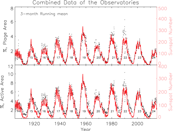
Figure 10. The black curve in the top panel of the figure shows the percentage of plage area determined after combining the measurements from spectroheliograms and filtergrams from KO, MWO, and PSPT (MLSO). The data represents the 3 month running average of the monthly mean of the percentage of the plage area. The overplotted red curve indicates the sunspot numbers for comparison. The bottom panel indicates the data for the percentage of the active area. The solar cycle number is also indicated in the figure.
Download figure:
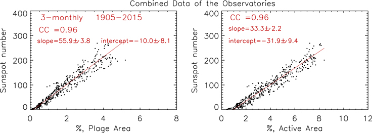
Standard image High-resolution imageThe left panel of Figure 11 shows the scatter plot of the sunspot numbers versus the derived percentage of plage area considering all of the data from KO, MWO, and MLSO on a monthly basis with a running average over 3 months, along with the linear fit. The right panel shows the scatter plot of the sunspot number versus active area. The CCs of 0.96 for both plots indicate that using the ECT methodology for Ca-K images, the derived results can be combined to generate a long time series of Ca-K data.
Figure 11. The left panel of the figure shows a scatter plot between the sunspot number and the percentage of plage area on a monthly basis with a running average over 3 months after ECT application for the KO, MWO, and MLSO data. The red line indicates the linear fit to the data. The right panel shows the plot of sunspot numbers vs. the percentage of the active area. The values of the correlation coefficient, slope, and intercept are shown in the panels.
Download figure:
Standard image High-resolution image
4. Summary and Discussions
The study of Ca-K data over a long time period provides details on chromospheric activity. In order to carry out such a study, uniform Ca-K data over a long time period, preferably from a single observatory, should be available. But, the data from a single ground-based observatory have data gaps, due to seasons, unavailability of observers, and working conditions of the instruments. In such a situation, it is advisable to combine the data from different observatories to obtain long-term data without gaps. However, the data obtained at different observatories have different spatial resolutions, bandpasses, scattered light in the telescope, properties of photographic plates/films, development methods, digitization instruments, etc. Hence, before combining these data together, it is essential to minimize these effects and make the data uniform over a long time period.
In order to do that, Singh et al. (2021) developed a methodology to make the contrast of the images the same for a large pool of data. They applied this methodology to all the data available at the KO (Singh et al. 2021). Once the contrast of the images is made the same, then the next step is to examine how well the methodology/technique can make the data obtained from different observatories uniform. Section 3 shows the way to test and compare different data sets after adjusting the contrast of each image. The analyses of Ca-K images by a number of authors using different methods show different percentages of plage areas (Worden et al. 1998; Chatzistergos et al. 2019; Priyal et al. 2019) for various data sets. Hence, we compared the Ca-K parameters with available long time series of sunspot data to find whether there is any correlation/anticorrelation or no relation with solar activity.
We find that the FWHM of the intensity distribution of the filtergrams is small compared to that of spectroheliograms. The FWHM of the intensity distribution determines the contrast of the images. The contrast of the Ca-K images depends on the passband of the filter or bandwidth of the exit slit of the spectroheliograph, spatial resolution of the telescope, emulsion used, electronic device, scatter in the instrument and sky conditions, etc. Different contrasts yield different values of the FWHM of the intensity distribution. The important point in ECT methodology is to maintain the FWHM of the intensity distribution of the image between 0.10 and 0.11 so that the contrast of the images in the time series becomes uniform.
We have applied the ECT technique to the KO, MWO, and PSPT data sets and made the contrast of the images uniform. We examined the uniformity in the data set by extracting chromospheric features such as plages and active areas. The intercomparison of the plage and active areas derived from ECT-applied KO and MWO spectroheliograms and KO and PSPT filtergrams shows good agreement. The Ca-K plage and active area for KO and MWO match very well before 1980, and after that, the KO data show a larger amplitude than MWO, but a smaller one than PSPT. The relative amplitudes of the combined KO, MWO, and PSPT Ca-K plage area agree very well with the sunspot number data from cycles 14–24.
5. Conclusions
The results obtained from measurements of the plage and active areas from KO and MWO spectroheliograms indicate that the ECT methodology can help combine similar data from different observatories to reduce the data gaps in the time series. The application of the ECT procedure to analyze the Ca-K images demonstrates that it makes the data from one or similar instruments almost of uniform quality by correcting the image contrast. Using the ECT-corrected long, uniform, time-series data, it will be possible to study short -and long-term variations reliably.
The amplitude of variation of the percentage of plage and active areas for different solar cycles appears correlated with the solar cycle strength when considering the sunspot numbers. This paper demonstrates that despite significant differences in observing properties (atmospheric seeing, telescope aperture, detector, film properties, etc.), the application of ECT allows a single homogenized data set to be created by combining data from different observatories. These data will be helpful for further reliable investigations of variations in the chromospheric activity and realistic modeling of the Sun.
We thank the reviewer for useful comments, which helped improve the content of the paper. We thank the numerous observers who have made observations, maintained the data at KO and MWO. We also thank the digitization teams at KO (lead by Jagdev Singh) and MWO. The high-spatial-resolution Ca-K data were downloaded from the Stanford Helioseismology Archive—prog:mwo (http://sha.stanford.edu/mwo/cak.html). The Precision Solar Photometric Telescope was maintained and operated at the Mauna Loa Solar Observatory from 1998 to 2015 by HAO/NCAR. The data were processed at and is served to the community by the Laboratory for Atmospheric and Space Physics, University of Colorado, Boulder (http://lasp.colorado.edu/pspt_access/). The sunspot data are from the World Data Center SILSO, Royal Observatory of Belgium, Brussels. Sunspot area data are downloaded from the website https://solarscience.msfc.nasa.gov/greenwch.shtml. The National Solar Observatory (NSO) is operated by the Association of Universities for Research in Astronomy (AURA), Inc., under a cooperative agreement with the National Science Foundation. Observations at the Mount Wilson Observatory have been supported over the years by the Carnegie Institute of Washington, the National Aeronautics and Space Agency, the US National Science Foundation, and the US Office of Naval Research. L.B. and A.A.P. are members of the international team on Modeling Space Weather And Total Solar Irradiance Over The Past Century supported by the International Space Science Institute(ISSI), Bern, Switzerland, and ISSI-Beijing, China.