


Abstract
Magnetic flux ropes, characterized as magnetic field lines that wrap and rotate around a central axis, are observed ubiquitously in the space-plasma environment. Accurately examining the physical parameters (e.g., axis orientation, helical handedness, current density, curvature radius, and size) of flux ropes is essential for studying their evolution and associated dynamics. The geometric parameters of flux ropes can be resolved by a cluster of at least four spacecraft with the separation scale much smaller than the flux ropes. However, most spacecraft missions are of single-point measurements, especially for the missions on other planets (e.g., Mars, Venus, Mercury), thus, the method for investigating the flux ropes based on single-point measurements becomes particularly important. A single-point method that infers the axis orientation of flux ropes was recently developed by Rong et al. Here, we apply this method to study two flux ropes observed by the Magnetospheric Multiscale Mission (MMS), one close to the force-free field and the other close to the non-force-free field, by comparing them with the multipoint analysis of MMS. Our study demonstrates that, apart from axis orientation, the method of Rong et al. can reasonably infer the current density, curvature radius of magnetic field, and the transverse size of flux ropes. We discussed the main error sources of calculated parameters, and suggest that it is worthwhile to widely apply the method by Rong et al. to single-point spacecraft missions for the purpose of examining the geometry and dynamics of flux ropes.
Export citation and abstract BibTeX RIS
1. Introduction
Magnetic flux ropes (MFRs), manifested as helical magnetic field lines wrapping around an axis, have been observed ubiquitously in the space-plasma environment, e.g., in Earth's magnetotail (e.g., Slavin et al. 2003a, 2003b; Zhang et al. 2007; Yang et al. 2014; Sun et al. 2019), Earth's magnetopause (e.g., Russell & Elphic 1979; Eastwood et al. 2016; Wang et al. 2017; Teh et al. 2017; Akhavan-Tafti et al. 2018), Mars' magnetotail (Hara et al. 2017), Venus's magnetotail (Zhang et al. 2012), Mercury's magnetotail (e.g., DiBraccio et al. 2015; Zhao et al. 2019), and interplanetary space (e.g., Burlaga 1988; Lepping et al. 1990). MFRs are generally considered as a product of magnetic reconnection that explosively release magnetic energy (e.g., Schindler 1974; Hones 1977; Wang et al. 2015; Eastwood et al. 2016; Zhou et al. 2017).
Accurate estimation of the physical parameters (e.g., axis orientation, current density, size, and curvature radius) of MFRs is vital for determining the magnetic geometry of MFRs and exploring their origin and evolution. This issue could be well solved by multipoint analysis with the advent of multispacecraft missions, e.g., the Cluster mission (Escoubet et al. 2001) and the Magnetospheric Multiscale mission (MMS; Burch et al. 2015), because the spatiotemporal variation of a magnetic field can be resolved by the simultaneous multipoint measurements of a spacecraft tetrahedron. The multipoint methods developed so far, such as the Minimum Directional Derivative (MDD; Shi et al. 2005, 2019), Multiple Triangulation Analysis (Zhou et al. 2006), and Magnetic Rotation Analysis (MRA; Shen et al. 2007) can derive the axis orientation by analyzing the spatial gradient of the magnetic field. As well as the axis orientation, the current density and curvature radius of MFRs could also be readily obtained by multipoint analysis, such as through the curlometer technique (Dunlop 2002), the Taylor expansion (Shen et al. 2003) and the MRA analysis by Shen et al. (2007). However, most current spacecraft missions, such as Geotail (Nishida 1994), ACE (Chiu et al. 1998), and the planetary missions, e.g., Mars Atmosphere and Volatile Evolution (MAVEN; Jakosky et al. 2015) and BepiColombo (Benkhoff et al. 2010), do not have a unique tetrahedral configuration like Cluster or MMS, and thus face a great challenge in inferring these parameters of MFRs.
In the past decades, with given assumptions, a few popular single-point methods have attempted to infer the axis orientation. (1) The minimum variance analysis based on magnetic field (BMVA; Sonnerup & Scheible 1998). It was argued that BMVA can infer the axis orientation relying on the calculated orthogonal eigendirections of magnetic field variation, and it does not require plasma data. However, model tests showed that the inferred axis orientation critically depends on the spacecraft's crossing trajectory (Moldwin & Hughes 1991; Xiao 2004; Rong et al. 2013); a different trajectory would result in different axis orientation. (2) The fit of force-free model (e.g., Lundquist 1950; Burlaga 1988; Lepping et al. 1990; Eastwood et al. 2016). This requires building a principle axis coordinate first based on BMVA and repeatedly fitting the data to the force-free model with least-squares analysis to find the final axis and the other model parameters. Nonetheless, one cannot guarantee that the real detected field structure of MFRs always fits well with the force-free model. Multipoint analysis of Cluster demonstrated that only the fraction around the centers of MFRs is close to the force-free field (e.g., Yang et al. 2014). (3) The technique of Grad–Shafranov reconstruction (GSR; Sonnerup & Guo 1996; Hau & Sonnerup 1999; Hu & Sonnerup 2001, 2002, 2003; Hu 2017; Hu et al. 2018). For the best GSR technique, an MFR is assumed to be in an approximately 2D magnetohydrostatic equilibrium (the balance between the gradient force of plasma pressure and the Lorentz force) during a spacecraft crossing, and a trial scheme is performed repeatedly to search for the axis orientation, for which the curve for total transverse pressure (plasma pressure plus magnetic pressure) versus the magnetic vector potential in the inbound crossing should be equal to that of the outbound crossing. This method could not only yield a reasonable axis orientation, but also the field distribution in the cross section of the MFR. However, applying the GSR technique increases the expense of a trial scheme, and it requires reliable plasma data, which is not always available for the spacecraft missions.
Recently, by assuming the radial magnetic field component is zero (Br = 0), Rong et al. (2013) presented a simple single-point method (we refer to it as R13) to derive the axis orientation of MFR. Model tests and application to the same MFR cases observed by the four spacecraft of Cluster demonstrated that R13 could infer the axis orientation consistently without the restriction of a force-free field configuration. Nonetheless, the typical separation scale of a Cluster tetrahedron is from several hundred kilometers to thousands of kilometers, which is comparable to or larger than the typical scale of MFRs observed in a magnetosphere. The multipoint analysis of Cluster on the field structure of MFRs could yield a significant truncation error owing to the large separation scale (e.g., Shen et al. 2003, 2007). Therefore, Rong et al. (2013) did not make the direct comparison between R13 and the multipoint analysis of Cluster. Moreover, there is no further analysis about the other parameters (e.g., current density, curvature radius, size) of MFRs by Rong et al. (2013).
In Table 1, we summarize the main constraints or assumptions of these single-point methods.
Table 1. The Summary of Various Single-point Methods in Analyzing MFRs
| BMVA | GSR | Fit of Force-free Field Model | R13 | |
|---|---|---|---|---|
| Required dataa | B | B, n, T, V | B, V | B, V |
| Key assumptions or constraints | Magnetic structure should be stationary | 2D magnetohydrostatic equilibrium, and the structure has an invariant direction | Force-free field model | Br = 0; magnetic structure should be stationary |
| Need a trial scheme? | No | Yes | Yes | No |
| Outcome | Three eigendirections which are sensitive to the spacecraft's trajectory | Axis and field distribution | Axis and model parameters | Axis and distance to axis center |
Notes.
aThe abbreviations B, n, T, V represent magnetic field, plasma density, plasma temperature, and plasma bulk velocity, respectively.Download table as: ASCIITypeset image
The four closer together spacecraft (separation scale 10 ∼ 20 km) of the MMS tetrahedron (Burch et al. 2015), with unprecedented temporal and spatial resolutions of magnetic field and plasma measurements, make it possible to evaluate the validity of R13 by comparison with the multipoint analysis. The high resolution of the magnetic field is measured by a fluxgate magnetometer operating at 128 vectors s−1 in burst mode (Russell et al. 2016). While fast plasma investigation (FPI) on board MMS can measure the electrons at a burst cadence of 30 ms and ions at a burst cadence of 150 ms, with an energy/charge range from 10 to 30,000 eV q−1. (Pollock et al. 2016). The plasma moments are derived from the all-sky electron and ion distributions by FPI.
As a continuation of Rong et al. (2013), here, we use R13 to analyze two flux rope cases which have been studied by previous studies (Eastwood et al. 2016; Zhao et al. 2016; Wang et al. 2017; Akhavan-Tafti et al. 2018). Through comparison with multipoint analysis methods and previous studies, we show that the single-point method, R13, apart from the consistent axis orientation, is also able to infer the current density, helical handedness, curvature radius, and boundaries of MFRs.
This paper is organized as follows: the method of R13 is briefly reviewed in Section 2; the overview of studied MFR cases by MMS, and the application results derived by the associated multipoint analysis and R13 are offered in Section 3; and the conclusion and discussion are finally given in Section 4.
2. Review of R13
Rong et al. (2013) presented a single-point method based on the sampled magnetic field data by spacecraft to infer the axis orientation of MFRs. This method makes two key assumptions: (1) the relative trajectory of the spacecraft crossing the MFR is straight; and (2) the magnetic field structure of MFRs is stable and the projected field along the axis can be seen as an ideal circular-like structure, or the radial field component is zero (Br = 0). The assumptions are usually acceptable, particularly for the innermost part of the MFR where the field structure is the least affected by the interaction with the ambient plasma. The available data are the relative velocity of spacecraft to cross the MFR, V, and the sampled magnetic field vector, B, by spacecraft. The unit vectors of relative velocity and magnetic field are  (
( = V/∣ V∣) and
  (
( = B/∣ B∣) respectively.
The first step in applying this method is to seek out the innermost location where the spacecraft, along its trajectory, is closest to the center of the MFR. In the cross section of the MFR, Figure 1(a) shows that v⊥ and  , the components of
  and
and  perpendicular to the axis orientation, respectively, would become parallel or antiparallel at the innermost location, and
  would reach the extremum. Hence, by checking the time series of
  , the data point of the innermost location could be identified. The identification of the innermost location is a key step in determining the axis orientation, because the axis orientation
  , the unit field direction at the innermost time
  , and
, and  should be coplanar there (see Figure 1(b)).
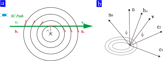
Figure 1. Two schematic views of MFR. (a) The variation of unit magnetic field direction along the trajectory of a spacecraft in the cross-sectional plane. The green arrow denotes the spacecraft trajectory, or it can be regarded as the direction of v⊥. The red arrows represent the direction of b⊥. r0, as the impact distance, is the closest distance to the center of MFR. (b) The geometric relationship between  and
and  .
.
Download figure:
Standard image High-resolution imageThe second step is to find the axis orientation  in the plane formed by
  and
and  . Using the derived
  , one can construct an orthogonal coordinate system
  to seek
  (see Figure 1(b)), where
In the plane constituted by  and
and  , the unsolved axis orientation
  deviates from
  by an angle of ψ. In other words,
  is a function of ψ. To constrain ψ, we noticed that the evaluated impact distance r0 (the closest distance of the center of the MFR to the spacecraft's trajectory) for each data point should be constant along the trajectory. The solved ψ or the optimal
  should result in a constant series of r0. Thus Rong et al. (2013) constructed a residue error as a function of ψ,

where M is the number of data points and  . The axis orientation
  can be numerically solved when σ2 reaches a minimum.
Here, to nondimensionalize the residue error, we suggest modifying Equation (2) as
It is worth mentioning that R13 can be still applied even if the magnetic field of MFR is varied along the axis direction, because R13 only assumes that the projected magnetic field vectors are azimuthally oriented in the cross section. Thus, R13 is superior to the 2D structure as assumed by, e.g., the fit of force-free model or GSR, at this point in the searching axis of MFRs.
With the optimal  derived from Equation (3), one can set up an orthogonal coordinate system
  , and associated cylindrical coordinates
  to describe the intrinsic helical field structure of the MFR, where
  (see Figure 1(b), V⊥ is the velocity component which is perpendicular to the axis,
  is the unit radial vector from the center of the MFR, and
  is the unit azimuthal vector. The cylindrical coordinate can be transformed from the orthogonal coordinate via
  and
and  , where the azimuth angle ϕ (0° ≤ ϕ ≤ 360°) rotationally increases from
  toward
  .
.
In the cylindrical coordinate, the current density and curvature radius could be further obtained if the magnetic field of the whole MFR is of a cylindrical azimuthal symmetry (Br = 0,  = 0,
= 0,  = 0). In this case, the axial and azimuthal components of current density can be calculated, respectively, as:
where μ0 is the vacuum permeability coefficient, r is the radial distance to the MFR's center, and Bn and Bϕ are the axial and azimuthal components of the magnetic field, respectively.
In this case, the curvature of the magnetic field line of the MFR ( ), whose full components are
can be also reduced to

where br, bϕ, and bn are the radial, azimuthal, and axial components of  , respectively.
3. Analysis of Cases
In this section, we apply R13 to study the magnetic structure of two MFR cases observed by MMS, the one is close to the force-free field and the other one is close to the non-force-free field. Comparison with other methods, particularly with multipoint methods, would highlight the validity and plausibility of R13. The system utilized here is the Geocentric Solar Ecliptic (GSE) coordinate system unless otherwise stated.
3.1. The Force-free Flux Rope Case
Figure 2 shows an ion-scale MFR case observed by MMS from 13:04:32–13:04:36 on 2015 October 16. MMS was located at (X = 8.33, Y = 8.51, Z = −0.7) RE, around the dayside magnetopause during this period, and the separation scale of the tetrahedron was about 20 km. This case, known as flux transfer events around the magnetopause, has been studied by many researchers (Eastwood et al. 2016; Zhao et al. 2016; Akhavan-Tafti et al. 2018).
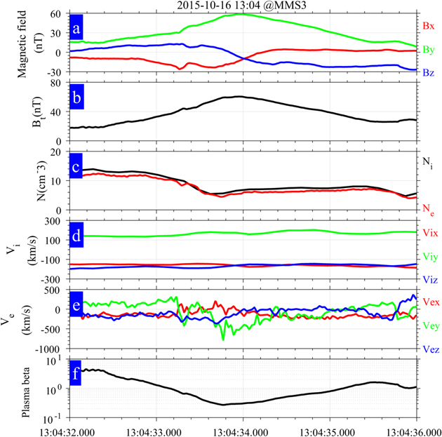
Figure 2. The flux rope case observed by MMS3 on 2015 October 16. From top to bottom, panels (a)–(f) show the time series of magnetic field components in GSE, the field strength, the number density of ions and electrons, the bulk velocity of ions and electrons in GSE, and the value of plasma beta.
Download figure:
Standard image High-resolution imageThe detected magnetic field data in Figure 2(a) shows bipolar signatures (−/+) for both Bx and Bz components accompanied by enhanced magnetic field strength and ion flow in the −Vz direction. These typical field signatures of MFRs suggest that MMS3 may have encountered a southward-moving MFR. The ion and electron number density evidence a slight decreasing tendency toward the MFR's center, from ∼14 to 5 cm−3, and the plasma beta (the ratio of plasma pressure to magnetic pressure) reaches a minimum around the center of an MFR. The signatures of both the magnetic field and plasma are consistent with those reported in previous studies of MFRs (e.g., Slavin et al. 2003a; Akhavan-Tafti et al. 2018; Sun et al. 2019).
3.1.1. Multipoint Analysis
Previous studies suggested that the scale of this MFR case is about several hundred kilometers (Eastwood et al. 2016; Akhavan-Tafti et al. 2018), which is larger than the scale of the MMS tetrahedron (∼20 km). Thus, the magnetic field within the tetrahedron could be better approximated by a linear varied field, which favors the application of multipoint analysis methods to examine the geometric structure of a magnetic field, e.g., axis orientation, current density, curvature radius of the magnetic field, etc. The parameters of field structure that are yielded could be treated as a benchmark for checking the validity of R13.
In this subsection, two popular multipoint analysis methods, i.e., MDD and MRA, are used independently to infer the axis orientation.
MDD can determine the dimensionality of magnetic structure and has been successfully applied to analysis of the structure of MFRs (Shi et al. 2005, 2019; Sun et al. 2019). The key step is to decompose the symmetrical matrix  , where ∇B is the gradient tensor of magnetic field. Three eigenvalues
  and the corresponding eigenvectors
  can be obtained by decomposing
  . The dimensionality of the magnetic structure can be indicated by the three eigenvalues. If magnetic structure is 1D, we would have
  , it would be
  if it is 2D.
Applying MDD to this case (see Figure 3(a)), we find  ∼ 0.35,
  ∼ 0.25, and
  ∼ 0.03 around the peak of the magnetic field. Thus, the MFR is a 2D structure, and the axis orientation is along
  (Shi et al. 2005, 2019). We select an appropriate time interval when
  is stable around the peak of the magnetic field (see the shaded interval "13:04:33.950–13:04:34.350" in Figure 3(b)). The mean of
  within this interval demonstrates that the axis orientation is (−0.2618, 0.9416, −0.2119).

Figure 3. Multipoint analysis of a flux rope. (a) Magnetic field, (b) the eigenvector corresponding to  in MDD, (c) the eigenvector corresponding to μ3 in MRA, (d) the current density derived by multipoint analysis of the magnetic field, (e) current density derived by plasma moments from FPI of MMS3, and (f) the angle between current density and the direction of the magnetic field.
Download figure:
Standard image High-resolution imageIn contrast to MDD, MRA is performed to analyze the spatial rotation rates of the magnetic field direction by decomposing the magnetic rotation tensor  (Shen et al. 2007). The decomposition of this tensor leads to three eigenvalues
  and three eigenvectors
  .
.  ,
,  , and
, and  represent the fastest, moderate, and slowest directions, respectively, along which the direction of magnetic field varies. Thus,
  is usually seen as the axis orientation of MFR when it was surveyed (Shen et al. 2007; Yang et al. 2014). The time series of calculated
  is displayed in Figure 3(c). With the same shaded interval in Figure 3(b), the average axis orientation derived by MRA is (−0.2679, 0.9338, −0.2373), which is nearly equal to that obtained by MDD. The inferred axis orientations from MDD and MRA are tabulated in Table 2.
Table 2. The Inferred Axis Orientations by Different Methods
| Spacecraft |

|

|

|
Method |
|---|---|---|---|---|
| MMS1 | (−0.77, −0.10, 0.63) | (0.60, 0.22, 0.77) | (−0.21, 0.97, −0.11) | R13 a |
| MMS2 | (−0.72, −0.02, 0.69) | (0.68, 0.17, 0.71) | (−0.14, 0.98, −0.11) | R13 |
| MMS3 | (−0.73, −0.04, 0.68) | (0.66, 0.21, 0.72) | (−0.18, 0.97, −0.13) | R13 |
| MMS4 | (−0.73, −0.05, 0.68) | (0.64, 0.30, 0.71) | (−0.24, 0.95, −0.19) | R13 |
| All | (−0.24, 0.95, −0.22) | MDD | ||
| All | (−0.25, 0.94, −0.23) | MRA | ||
| MMS3 | (−0.01, 0.99, −0.15) | Fitting of force-free modelb | ||
| All | (−0.26, 0.90, −0.36) | MVA on the gradient of magnetic pressurec |
Notes.
a R13 is the single-point method presented by Rong et al. (2013). bThe fitting of the force-free model applied by Eastwood et al. (2016). cThe minimum variance analysis on the gradient of magnetic pressure employed by Zhao et al. (2016).Download table as: ASCIITypeset image
According to  , the current density can be derived based on a multipoint analysis on a magnetic field gradient using Taylor expansion by Shen et al. (2003) (referred to as S03). The calculated current density is shown in Figure 3(d). Alternatively, with plasma moments measured by FPI on board each MMS, one can calculate the current density with plasma measurement. Figure 3(e) shows the current density calculated by
  with the plasma measurement of MMS3 (see also Eastwood et al. 2016), where ne is the number density of electrons, while Vi and Ve are the bulk velocity of protons and electrons respectively. Note that to keep a consistent time resolution with the magnetic field, the plasma moments in calculating current density have been interpolated with the cadence of magnetic field data (128 s−1).
Apparently, the two methods to calculate the current density show a good agreement, demonstrating that the measurement of plasma moments by FPI can be employed to calculate the current density, and that the electrons are the main current carrier of this MFR (not shown here). It is interesting to note that there is a significant field-aligned current in the center of the MFR and a filament peak of current ahead of it, suggesting that the magnetic field is nearly force-free around the center but non-force-free in the outer region of the MFR.
The angle between current density and magnetic field, denoted as γ, is nearly equal to 0° in the center and trail of the MFR (see Figure 3(f)), which indicates that the current density is basically field-aligned, and suggests that the field structures in the MFR's center and trail are close to the force-free field with a right-hand helical handedness (Eastwood et al. 2016).
3.1.2. Application of R13
We now perform R13 to analyze the field structure of this flux rope. Without loss of generality, we arbitrarily choose the data provided by MMS3 for our analysis.
Following the procedures of Rong et al. (2013), we identify the innermost time first by checking the time series of  . Considering the much slower velocity of the spacecraft (∼2 km s−1) , the velocity of the MFR can be seen as VHT which is the velocity of the DeHoffmann–Teller (HT) frame (Khrabrov & Sonnerup 1998), if the encountered flux rope is a quasi-stationary magnetic structure (for this case, using the multipoint analysis of MMS, Zhao et al. (2016) have demonstrated that the magnetic curvature force is balanced by the magnetic pressure force, and the plasma pressure gradient is relatively much smaller). With HT analysis within the interval 13:04:32–13:04:36, the relative velocity of the spacecraft to the MFR is calculated as
  = (167.88, −208.83, 165.94) km s−1. The correlation coefficient ∼0.998 between
  and
and  (V is the bulk ion velocity from FPI) guarantees the reliability of HT analysis. As a result, the unit vector of
  is derived as
  = (0.5327, −0.6626, 0.5265).
Figure 4(a) shows the time series of  . Clearly, the product of
  reaches a minimum around the peak of field strength (Figure 4(b)). Thus, corresponding to the minimum of
  , the time when the spacecraft is located at the innermost part or is closest to the MFR's center can be identified at 13:04:33.982 (see the red dashed lines in Figures 4(a) and (b)). Accordingly, having identified the innermost time, the inferred
  is (−0.7295, −0.0442, 0.6825),
  is (0.4290, 0.7477, 0.5069), and the local coordinate system
  can be constructed via Equation (1).
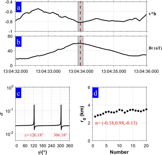
Figure 4. Analysis of a flux rope based on the single-point method proposed by Rong et al. (2013). (a), (b) The time series of  and the magnetic field strength, respectively. The red dashed lines mark the time when
  reaches a minimum. (c) The variation of σ against ψ. (d) The evaluated impact distances for the 20 data points of magnetic vectors.
Download figure:
Standard image High-resolution imageWe choose a short interval centered around the innermost time with 20 sampled magnetic field vectors to infer the axis orientation (a longer interval may contain the samples near the boundary where field structures are significantly distorted). It should be noted that, as suggested by Rong et al. (2013), the sampled data point at the innermost time has been excluded to avoid a poor calculation because the evaluated impact distance (r0) would become infinite in this time (see Equation (9) of Rong et al. 2013). By numerical calculation, we find that the residue error σ, defined in Equation (3), would reach a minimum ( = 0.015) when the angle between
  and
and  equals either 126
 18 or 30618 (Figure 4(c)), which, in principle, results in a pair of antiparallel axis orientations. Following Rong et al. (2013), we choose the one pointing roughly along
  as the final axis orientation. As a result, the axis orientation
  is derived as (−0.1767, 0.9762, −0.1257), and
  is estimated as (0.6607, 0.2123, 0.7200). In other words, projected along the derived
  , the orientations of the 20 magnetic vectors in trajectory can be best fitted with a circular-like field structure. We find the mean impact distance of the trajectory is about ∼3.2 km (see Figure 4(d)), which indicates that, in this case, MMS3 was almost crossing the center of the MFR.
Since  ,
,  , and
, and  are inferred, the orthogonal coordinate system
  is set up to describe the intrinsic helical field structure of the MFR. In this coordinate, Figure 5(a) shows the projection of sampled b (within the shaded interval) in the cross section. Obviously the loop-like pattern of the projected field (also see Figure 5(b)) is consistent with the field-aligned current density near the center of the MFR (see Figure 3(c)), which demonstrates the validity of R13.
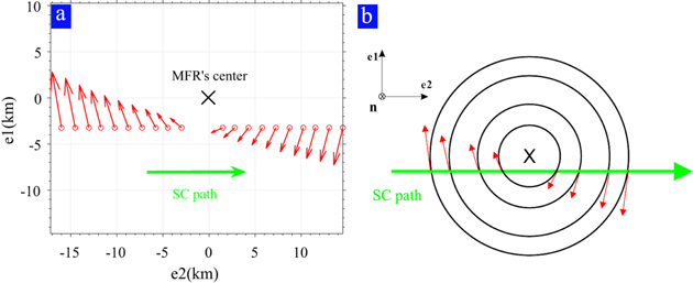
Figure 5. (a) The projection of unit field vectors of sampled data points on the  plane. The red arrows represent the orientations of b⊥, and the green arrow represents the relative moving direction of the spacecraft crossing the MFR. The origin, marked as "×," represents the center of the MFR. (b) A sketched diagram of the spacecraft crossing the MFR.
Download figure:
Standard image High-resolution imageRepeating the same procedure as conducted above, the axis orientations of this MFR based on the measurements of MMS1, MMS2, and MMS4 are also inferred separately. The yielded results are tabulated in Table 2. As a comparison, the axis orientations by means of MDD, MRA, and the fitting of the force-free model (Eastwood et al. 2016), and a minimum variance analysis on the gradient of magnetic pressure (Zhao et al. 2016) are also tabulated in Table 2. In contrast to the single-point fitting method used by Eastwood et al. (2016), it seems the axis orientation inferred by R13 is closer to the axis orientation estimated by multipoint methods, i.e., MDD, MRA, and the analysis of magnetic pressure gradient by Zhao et al. (2016).
With the derived coordinate system  for each spacecraft, we can examine the current density and the curvature radius of the magnetic field for associated cylindrical coordinates
  based on Equations (4)–(6), respectively. The time series of the calculated axial component, jn, the azimuthal component, jϕ, and the radial component jr of current density for MMS1, MMS2, MMS3, and MMS4 are shown in Figures 6(a)–(d), (e)–(h) and (i)–(l), respectively. The angle between the current density and magnetic field, denoted as γ, is shown in Figures 6(m)–(p) for the four spacecraft.
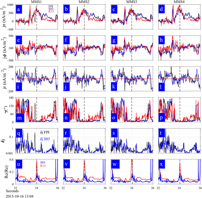
Figure 6. The current density and curvature radius of the MFR. The inferred axial components (jn) of current density for four spacecraft are shown in (a)–(d), the azimuthal components (jr) of current density are shown in (e)–(h), the radial components (jr) of current density are shown in (i)–(l), the angles between the current density and local magnetic field direction are shown in (m)–(p), the relative errors of the calculated current density are displayed in (q)–(t), and the inferred curvature radii of magnetic field are shown in (u)–(x). In these panels, the red and black lines represent the single-point results by R13 and plasma moment of FPI, respectively. The blue lines represent the results of multipoint analysis by S03, which is the same for all panels in each column. The black dashed lines in all panels denote the time when the spacecraft is closest to the center of MFR.
Download figure:
Standard image High-resolution imageIn comparison to the current density calculated by  and
and  by S03 (because we cannot judge which one could be better seen as the benchmark of current density, both are shown for reference), we find that the current density calculated by R13 for each of the four spacecraft are consistent with that derived from the plasma moments and the curl of magnetic field. Note that the axial, azimuthal, and radial components of both j = ne e(Vi − Ve) and
  are calculated based on the cylindrical coordinates
  inferred by R13. The consistent pattern of axial and azimuthal components of current density demonstrates that R13 can recover the distribution of current density the MFR (red line) by means of a one-point analysis. Furthermore, the derived radial component of current density, jr, by S03 and FPI is always nonzero, which indicates that
  for the MFR. Thus, to evaluate the calculation quality of current density by R13, we could calculate the relative errors of current density derived by R13 (Figures 6(q)–(t)) as
  (
( ) if the current density derived by FPI (S03) is regarded as the accurate value, where
  ,
,  , and
, and  are the calculated strength of current density by FPI, S03, and R13, respectively. One can find that
  and δj < 0.2 in most parts of the MFR, especially in the center of the MFR, which demonstrated that the current density derived by R13 is reasonable.
The curvature radius of the magnetic field is calculated separately for each of the four spacecraft via Equation (6), as shown in Figures 6(u)–(x). For comparison, the curvature radius calculated by S03 is displayed. It is clear that the curvature radius from S03 is larger in the center of an MFR (∼0.25 RE) than in the outer region (∼0.05 RE), which implies that magnetic field lines become straighter in the center of the MFR. This is consistent with previous studies (e.g., Shen et al. 2007; Yang et al. 2014). It is interesting to note that R13 obtains a similar pattern of curvature radius variation, but slightly overestimates the curvature radius. Because R13 ignores axial and azimuthal components and only estimates the radial component of curvature, the real curvature (curvature radius) is underestimated (overestimated). The discrepancy demonstrates that the actual field structure in the inner core of the MFR cannot be an ideal structure of cylindrical azimuthal symmetry.
With the derived axis orientation by R13, we could further study the helical field structure of the MFR, and identify its boundaries or transverse size.
In the cross section near the center of the MFR (Figure 7(a)), the projected magnetic field would be close to a circular configuration, and the displacement vector (r, cyan lines) should be nearly perpendicular to the magnetic field vector (b⊥, red arrows). The angle  , defined as
  , is presumably close to 90° around the center of the MFR where the cross section of the MFR is nearly circular (Br ≈ 0). In contrast, in the outer part or boundary,
  would deviate from 90° due to the distorted field structure or nonnegligible Br component induced by the interaction with ambient plasma. Thus, the boundaries of MFRs could be identified to some extent by checking the time series of
  . The time series of
  recorded by MMS3 is shown in Figure 7(b). As expected, during the passage of an MFR by the spacecraft,
  increases when the spacecraft moves toward the center of the MFR, stays about 90° when around the inner part, and finally decreases as it moves away from the MFR.

Figure 7. (a) A sketched diagram of the MFR, (b) the angle between the displacement vector and the direction of magnetic field (see the definition in the text), (c) the helical angle, (d) the strength of the magnetic field and the axial component of the magnetic field derived from R13, (e) the angle between current density and orientation of the magnetic field, (f) the force-free factor α. The shaded interval represents the period of crossing the flux rope. The black dashed line shows the time when the spacecraft is closest to the center of the MFR.
Download figure:
Standard image High-resolution imageFurther, one can define a helical angle as  , where B⊥
  is the field component perpendicular to the axis, to study the helical geometry of the MFR's field. Since the magnetic field in the center of the MFR is nearly parallel to the axis orientation, one would expect an increased helical angle when the distance to the center of the MFR is decreased. Figure 7(c) shows the calculated helical angle by R13 during the whole passage of the MFR. For comparison, according to the axis orientation inferred from MRA, the helical angle from multipoint analysis is also displayed. The two methods yield an almost coincident time series of the helical angle, suggesting the validity of the derived axis orientation by R13. In line with our expectations, we find the calculated helical angle increases as the spacecraft approaches the innermost location, and decreases as it moves away from the MFR. The maximum helical angle of nearly 90° demonstrates that the field lines around the innermost part are almost parallel to the axis orientation.
Therefore, considering the variation of  , the helical angle, and the axial component of magnetic field and field strength (Figure 7(d)), we suggest that the turning points (the minimum value of
  ) on both sides of the center of the MFR (13:04:32.708 and 13:04:35.404), should correspond to the inbound and outbound crossing time of MFR boundaries, respectively. Thus the interval of crossing the MFR is about 2.7 s (see the shaded interval in Figures 7(b)–(f)). It is worth noting that with our identification of the boundaries, the frontal region or outer draping region with the non-force-free field could be reasonably included within the MFR (Figure 7(e)).
With the knowledge of axis orientation and the relative velocity of the spacecraft ( ), the transverse speed of the crossing spacecraft is
  =186 km s−1; thus the diameter (radius) of the MFR is about 502 km (251 km). Since the radius of a cylindrical MFR is approximated to be the curvature radius of projected field lines on the cross section near the boundaries, one could check the accuracy of the identified MFR's boundaries in terms of the curvature radius. Considering that the curvature radius is about 0.05 RE, or 319 km near the boundaries of the MFR (13:04:32.5–13:04:33 or 13:04:34.5–13:04:35) (see Figures 6(m)–(p)), and the helical angle is about 45° there, the radius of the MFR could be 319 × cos(45°) ≈ 226 km, which is comparable to that estimated by
  . Thus the boundaries we identified by
  are reasonable. In contrast, with the fit of the force-free model, the radius of an MFR estimated previously by Eastwood et al. (2016) and Akhavan-Tafti et al. (2018) is about 400 ∼ 550 km, about twice that of our estimation.
In the innermost part of this MFR, which has a low beta (∼0.25) and a dominated field-aligned current (see Figures 2(f) and 7(e)), the innermost field basically satisfies the force-free field (Lepping et al. 1990; Yang et al. 2014),  . The calculated force-free factor α (
 ) demonstrates that α is nearly constant (∼0.013 km−1) in the innermost position of the MFR, suggesting a linearly force-free field there (Figure 7(f)).
Repeating the same procedures, the radii of MFRs based on the measurements of MMS1, MMS2, and MMS4 are also inferred separately. The results yielded are tabulated in Table 3.
Table 3. The Inferred Radius of the MFR
| Spacecraft | Intervalb | V⊥ (km s−1) | R (km)c | Method |
|---|---|---|---|---|
| MMS1 | 13:04:32.808–13:04:35:590 | 186.42 | 259 | R13 d |
| MMS2 | 13:04:32.736–13:04:35:572 | 199.95 | 284 | R13 |
| MMS3 | 13:04:32.708–13:04:35:404 | 186.06 | 251 | R13 |
| MMS4 | 13:04:32.784–13:04:35.409 | 155.58 | 204 | R13 |
| MMS3 | ∼ | ∼ | 550 | Fit of force-free modele |
| ∼a | ∼ | ∼ | 431 | Fit of force-free modelf |
Notes.
aThe symbol "∼" means that the related information is unclear. bThe duration of crossing the MFR based on the variation of .
cThe radius of the MFR.
d
R13 is the same as defined in Table 2.
eThe fit of the force-free model by Eastwood et al. (2016).
fThe fit of the force-free model by Akhavan-Tafti et al. (2018).
.
cThe radius of the MFR.
d
R13 is the same as defined in Table 2.
eThe fit of the force-free model by Eastwood et al. (2016).
fThe fit of the force-free model by Akhavan-Tafti et al. (2018).
Download table as: ASCIITypeset image
Using the inferred axis orientation and the transverse size of the MFR based on the measurements of MMS3, we project the field vectors recorded by four spacecraft on the cross section in Figure 8. The projected magnetic field is circular-like or close to the structure of azimuthal symmetry near the center (see Figure 8(b)), but it is distorted or deviates from the circular-like shape near the boundaries. Furthermore, note that to the left of the center (∼−110 km), there is a jump/transition of the projected magnetic field, which is consistent with the peak filament current as reported by Eastwood et al. (2016).
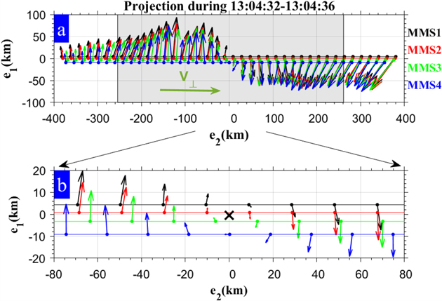
Figure 8. The projection of b⊥on the cross section of the flux rope. The resampled field vectors with a cadence of 0.1 s as recorded by MMS1, MMS2, MMS3, and MMS4 are labeled in black, red, green, and blue, respectively. The inferred size of the MFR is shaded. (b) Enlargement of the projection of magnetic field vectors near the center of the MFR, which is labeled by a cross.
Download figure:
Standard image High-resolution image3.2. The Non-force-free Flux Rope Case
The above subsections show a successful application of R13 to an MFR case with a nearly force-free field in the core. In this section, we continue to show that R13 can be also applied to study the field structure of a non-force-free MFR if the assumption of cylindrically azimuthal symmetry holds. The non-force-free case we studied here was observed by MMS in the magnetotail at 17:42 on 2017 July 20, which was reported by Sun et al. (2019).
At that time, MMS was located at [X = −23.75, Y = 5.5, Z = 5.04] RE. The recorded bipolar variation of Bz and enhancement of By components by spacecraft (Figure 9(a)), suggest there was an encounter with an MFR. Due to the small separation distance of the MMS tetrahedron (scale less than 19 km), we only consider the data of MMS3 for performing the single-point analysis by R13.
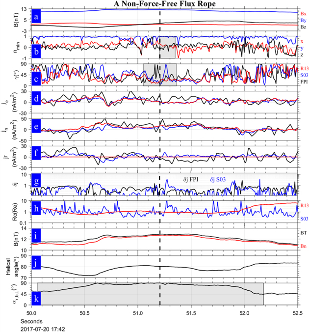
Figure 9. A non-force-free flux rope observed by MMS3 during 2017 July 20 17:42:50.0–52.5. (a) The variation of magnetic field, (b) the eigenvector corresponding to  in MDD, (c) the angle between current density and magnetic field, (d) the time series of azimuthal current density derived by S03, FPI, and R13, (e) the time series of axial current density, (f) the time series of radial current density derived by S03 and FPI, (g) the relative error of current density, (h) the radius of magnetic curvature obtained by S03 and R13, (i) the strength of the magnetic field and the axial component of magnetic field derived from R13, (j) the helical angle, and (k) the angle of
  , where the interval of crossing MFR is shaded. The black dashed lines in each panel denote the time (17:42:51.207) when MMS3 was crossing the innermost position of the MFR.
Download figure:
Standard image High-resolution imageWe have taken three different methods to infer the axis orientation of this MFR. (1) The BMVA over the whole interval 17:42:50.0–17:42:52.5 yields the intermediate variance direction (−0.084, 0.996, 0.03). (2) The MDD analysis around the center of the MFR (shaded interval 17:42:51.2–17:42:51.35 in Figure 9(b)) yields the mean axis orientation (0.0873, 0.9945, 0.0571). (3) Using the obtained VHT = [367.89, −64.79, 58.88] km s−1, the analysis of R13 based on the data of MMS3 around the center of the MFR (shaded interval 17:42:51.05–17:42:51.36 in Figure 9(c)) yields the axis orientation (0.023, 0.985, 0.173), and the evaluated mean impact distance  km.
km.
By repeating the same procedures as done in Section 3.1, we show the comparison of derived results between R13 and the multipoint methods (MDD and S03) in Figure 9. In contrast to the above case, the angle γ calculated with different methods in Figure 9(c) indicates that the current density is not significantly field-aligned, even around the innermost position of the MFR (γ ∼ 30°, and even reaches 90°). Thus, this MFR should be a non-force-free case with a right-hand helical handedness.
The azimuthal and axial components of current density,  and jn, derived by FPI, S03, and R13 basically have the same variation pattern (see Figures 9(d) and (e)). Note that due to the errors of plasma measurement, e.g., the contamination of secondary electrons generated via photoemission from the sunlit spacecraft and instrument surfaces in the magnetotail plasma sheet (Gershman et al. 2017), the current density derived by FPI shows some differences with that derived by S03. Thus, the current density derived by S03 is better seen as the benchmark. It is interesting to note that the derived jϕ and jn by our R13 are almost coincident with that derived by S03. The radial current derived by S03 (Figure 9(f)) is basically lower than 10 nA m−2, while the relative error of the current density (Figure 9(g)) is lower than 0.5 in most parts of the MFR. Thus, the current density derived by R13 for this case is reasonable.
Meanwhile, we find the calculated curvature radius by R13 (Figure 9(h)) basically agrees with that derived by S03 around the innermost position of the MFR (about 1 RE), but shows significant discrepancy far away from the innermost position, which again implies that the assumption of cylindrical azimuthal symmetry makes sense in the innermost part for this MFR.
The variation of the axial component of magnetic field (Figure 9(i)) and the helical angle of magnetic field (Figure 9(j)) suggest that the magnetic field in the MFR is dominated by the axial component.
Based on the variation of  as shown in Figure 9(k), the inbound and outbound crossings of the MFR's boundary are identified at 17:42:50:055 and 17:42:52.179, respectively. Considering that the perpendicular speed of VHT is approximately 375.5 km s−1 and the mean impact distance is 11.1 km, the diameter (radius) of this MFR is estimated at about 797.87 km (398.94 km), which is slightly smaller than that inferred by timing analysis (about 942 km). It is interesting to note that the projection of the curvature radius around the boundaries (∼0.8 RE from S03, shown in Figure 9(f)) with the helical angle (84°) yields a comparable radius of about 533 km. Thus, the identification of boundaries based on the variation of
  still makes sense for the non-force-free MFR case.
In summary, the assumption of cylindrical azimuthal symmetry is reliable for fitting the interior field structure of this non-force-free MFR case, particularly around the innermost position of the MFR. The calculated axis orientation, current density, curvature radius of the magnetic field, and the identified boundaries of the MFR by R13 are basically consistent with the results of multipoint analysis.
4. Conclusion and Discussion
In this paper, by applying R13 to two MFRs observed by the MMS tetrahedron, we analyze the magnetic field structure of flux ropes. The parameters for characterizing the field structure, including the axis orientation, current density, curvature radius of the magnetic field, and the transverse size, are estimated by R13 under the assumption of cylindrical azimuthal symmetry of the MFR. The comparison with the multipoint analysis methods demonstrates that the parameters inferred by the single-point analysis of R13 are reasonable regardless of whether the flux rope is quasi-force-free field or not.
Although R13 is reliable and applicable, the points below should be noted to interpret the error sources of its derived parameters.
- 1.To infer the axis orientation, R13 requires that the projected field vectors in the cross section should be azimuthally oriented for the best, i.e., Br ∼ 0. As stated by Rong et al. (2013), the assumption could be valid when sampled data are confined around the innermost position of the MFR because the field structure there is less affected by the interaction with ambient plasma. The two studied cases here show that the axis orientation inferred by R13 around the innermost position indeed agrees well with that by the multipoint analysis of MMS. However,the field structure around the innermost part of an MFR cannot have an ideal Br ∼ 0. The deviation error from Br ∼ 0, or the error of axis inferred by R13, can be indicated by the nonzero minimum σ (see Equation (3) and Figure 4(c)).
- 2.As indicated by Equations (4) and (6), if the magnetic field for the whole MFR is further assumed to be of cylindrical azimuthal symmetry (Br ∼ 0,
 = 0, = 0), the current density and curvature radius could be evaluated, respectively. It is relatively easy to check the validity of Br ∼ 0 by the variation of , because is also equal to , which inversely varies with Br. Obviously, Br ∼ 0 is well satisfied around the innermost position of MFRs, but it becomes significant around the boundaries as indicated by in the two studied MFR cases.
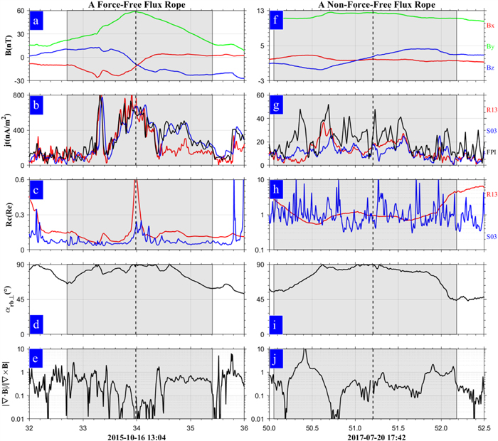
 - 3.However, the way to evaluate the validity of = 0 is challenging for single-point analysis. Because the three cylindrical coordinates of a spacecraft's location are varied simultaneously along the trajectory, it is impossible to accurately separate the gradient components associated with and . Considering , one could calculate to represent the divergence of the magnetic field, or the error induced by , where Br, though it is minor, is the radial field component in the cylindrical coordinates setup by R13. Consequently, we could construct a dimensionless parameter to roughly indicate the error brought by , which is similar to the indicator developed by Dunlop (2002) to evaluate the calculation error of current density. The calculation of is based on Equation (4). In Figures 10(e) and (j), under the assumption of = 0, we calculate for the two studied flux ropes. It is clear that the calculated for both cases shows a dip around the innermost position, which demonstrates that our calculations of current density and curvature radius by R13 are relatively reasonable there. We noticed that when becomes larger, e.g., >0.5 far away from the innermost position, the difference in calculated current density and curvature radius with the multipoint analysis becomes significant.


Figure 10. The error estimation for the two studied MFR cases. From top to bottom: (a), (f) the variation of magnetic field, (b), (g) the magnitude of current density, (c), (h) the curvature radius of magnetic field, (d), (i) the variation of  , and (e), (j) the variation of
  . The black dashed line in each panel labels the time when spacecraft is at the innermost part of the MFR, and the interval for crossing the flux rope is shaded.
Download figure:
Standard image High-resolution image
In summary, the comparison with multipoint analysis methods for two flux rope cases demonstrates that the single-point analysis of R13 is reasonable in analyzing the interior field structure of MFRs unless it is highly distorted. Therefore, R13 could be applied widely to the "big data set" accumulated by the single-point spacecraft missions in history, and to the planetary missions, e.g., MAVEN (Jakosky et al. 2015) and the BepiColombo mission (Benkhoff et al. 2010), to study the geometry of MFRs and explore their origin, evolution, and roles in the planetary space environment. Nonetheless, the application of R13 strongly depends on the assumption of cylindrical azimuthal symmetry, and the yielded parameters by R13 must always be interpreted with caution, and may combine the technique of GSR if necessary.
The magnetic field data and plasma data of MMS used in this paper are available from the MMS Science Data Center at http://lasp.colorado.edu/mms/sdc/. The authors are grateful to the entire MMS team for providing the data. This work is supported by the Strategic Priority Research Program of the Chinese Academy of Sciences (grant No. XDA17010201), the Key Research Program of the Institute of Geology & Geophysics, CAS, grant No. IGGCAS- 201904, the National Natural Science Foundation of China (grants 41922031, 41774188, 41874190, 41874176) and NASA MMS Guest Investigator grant 80NSSC18K1363. We thank Weijie Sun, Shutao Yao, Shimou Wang, Kai Fan, Wenya Li, Nanqiao Du, Zhen Shi, Xinzhou Li, Di Liu, and Fang Qian for providing helpful suggestions.