


Abstract
The search for new global scaling relations linking the physical properties of galaxies has a fundamental interest. Furthermore, their recovery from spatially resolved relations has been in the spotlight of integral field spectroscopy (IFS). In this study, we investigate the existence of global and local relations between stellar age (Age⋆) and gas-phase metallicity (Zg). To this aim, we analyze IFS data for a sample of 736 star-forming disk galaxies from the MaNGA survey. We report a positive correlation between the global Zg and D(4000) (an indicator of stellar age), with a slope that decreases with increasing galaxy mass. Locally, a similar trend is found when analyzing the Zg and D(4000) of the star-forming regions, as well as the residuals resulting from removing the radial gradients of both parameters. The local laws have systematically smaller slopes than the global one. We ascribe this difference to random errors that cause the true slope of the Age⋆–Zg relation to be systematically underestimated when performing a least-squares fitting. The explored relation is intimately linked with the already known relation between gas metallicity and star formation rate at fixed mass, both presenting a common physical origin.
Export citation and abstract BibTeX RIS
1. Introduction
The modeling of galaxies formed in a cosmological context has reached an impressive degree of realism (e.g., Ceverino et al. 2014; Hopkins et al. 2014, 2018; Vogelsberger et al. 2014, 2020; Schaye et al. 2015; Springel et al. 2018; Nelson et al. 2019). Model galaxies are able to reproduce many of the observed scaling relations (e.g., the distribution of masses, luminosities, and sizes or the increase of star formation rate (SFR) and metallicity with mass), as well as the properties of individual galaxies like the Milky Way or Andromeda (e.g., Nuza et al. 2014; Scannapieco et al. 2015; Grand et al. 2018, 2019; Carigi et al. 2019; Buck et al. 2020). However, this successful modeling is not free from tune-up. Simulations cannot self-consistently resolve all of the relevant physical scales, from individual stars to cosmological volumes. Subgrid physics is required to account for key processes like transforming gas into stars or supernova feedback (e.g., Schaye & Dalla Vecchia 2008; Dalla Vecchia & Schaye 2012; Marinacci et al. 2019; Terrazas et al. 2020). The free parameters encrypting such subgrid physics are tuned to reproduce some of the observed scaling properties (e.g., the distribution of luminosities or stellar masses), whereas other scaling relations are used to evaluate the consistency of the simulated galaxies (Crain et al. 2015; Sánchez Almeida & Dalla Vecchia 2018; Genel et al. 2018; Torrey et al. 2019). Testing against scaling relations represents the best benchmark available to judge the realism of the numerical simulations and, consequently, the way to assess our understanding of how galaxies form and evolve. Thus, investigations to disclose and characterize new galaxy scaling relations are essential.
One scaling relation that has received notable attention is called the fundamental metallicity relation (FMR; Ellison et al. 2008; Lara-López et al. 2010; Mannucci et al. 2010). In general, more massive galaxies have larger gas-phase metallicity (Zg
) and SFR. However, this trend of increasing Zg
with increasing SFR reverses when galaxies of the same stellar mass M⋆ are compared (provided ![$\mathrm{log}[{M}_{\star }/{M}_{\odot }]\lt 10.5$](https://content.cld.iop.org/journals/0004-637X/903/1/52/revision3/apjabba7cieqn1.gif) ). The FMR shows that those galaxies with larger SFR have smaller Zg
. There is evidence for the FMR to hold until at least redshift 3 (e.g., Troncoso et al. 2014; Sánchez Almeida 2017), but there are also dissenting views, mostly on whether the SFR is truly needed to describe the relation between M⋆ and Zg
(Izotov et al. 2014; de los Reyes et al. 2015; Sanders et al. 2015; Sánchez et al. 2013, 2017, 2019b; Barrera-Ballesteros et al. 2017). The FMR is taken as evidence for metal-poor cosmic gas accretion fueling star formation (e.g., Mannucci et al. 2010; Brisbin & Harwit 2012; Davé et al. 2012), an observationally elusive but fundamental physical process according to numerical simulations (e.g., Dekel et al. 2009; Sánchez Almeida et al. 2014).
). The FMR shows that those galaxies with larger SFR have smaller Zg
. There is evidence for the FMR to hold until at least redshift 3 (e.g., Troncoso et al. 2014; Sánchez Almeida 2017), but there are also dissenting views, mostly on whether the SFR is truly needed to describe the relation between M⋆ and Zg
(Izotov et al. 2014; de los Reyes et al. 2015; Sanders et al. 2015; Sánchez et al. 2013, 2017, 2019b; Barrera-Ballesteros et al. 2017). The FMR is taken as evidence for metal-poor cosmic gas accretion fueling star formation (e.g., Mannucci et al. 2010; Brisbin & Harwit 2012; Davé et al. 2012), an observationally elusive but fundamental physical process according to numerical simulations (e.g., Dekel et al. 2009; Sánchez Almeida et al. 2014).
Often, the global scaling relations, where each galaxy is a point, can be recovered from spatially resolved relations (e.g., Rosales-Ortega et al. 2012; Sánchez et al. 2013; Wuyts et al. 2013; Barrera-Ballesteros et al. 2016; Cano-Díaz et al. 2016; Hsieh et al. 2017; Erroz-Ferrer et al. 2019). Sánchez Almeida & Sánchez-Menguiano (2019, hereafter SA19) showed that the FMR results from the spatial integration of a local correlation between an excess of Zg and an excess of surface SFR. Indeed, Sánchez-Menguiano et al. (2019, hereafter SM19) observed such a local (anti)correlation analyzing spatially resolved MaNGA galaxies, and similar conclusions are also drawn using other approaches and data sets (Sánchez Almeida et al. 2018; Hwang et al. 2019). Given a number of simplifying assumptions (e.g., small relative fluctuations), SA19 derived the mathematical equivalence between the global and local correlations, which are predicted to have exactly the same logarithmic slope. Since it is a formal derivation, the relation still holds even when the variables are renamed, leading to the conclusion that the correspondence between local and global laws is not specific to the FMR. This fact implies that there should be local counterparts associated with other known global scaling relations involving Zg . In particular, the stellar age has been shown to be correlated with Zg . For a set of local analogs to Ly-break galaxies, systems with younger stellar populations have lower Zg at fixed M⋆ (Lian et al. 2015). The existence of this global correlation involving stellar age (Age⋆) suggests the existence of a corresponding local counterpart, namely, a local correlation between Zg and Age⋆. This paper describes our work to disclose and characterize this foretold relation using the same MaNGA data set employed in SM19.
The paper is organized as follows. Section 2 briefly describes the MaNGA data and the galaxy sample, whereas the procedures to compute the physical parameters used in the analysis are given in Section 3. The derivation of the galaxy-integrated correlation (global law) is included in Section 4, with the local law worked out and characterized in Section 5. Local and global correlations are compared in Section 6. Finally, the results are discussed in Section 7. Supplementary material includes Appendices A–C. Appendix A presents several tests performed to assess the robustness of the results. Appendix B analyzes the Zg versus Age⋆ relation when ages are computed from fitting the stellar continuum. Lastly, Appendix C shows how the slope of a relation is underestimated when using noisy data, a conclusion we employ to justify some of the results.
2. Data and Galaxy Sample
2.1. MaNGA Data
Mapping Nearby Galaxies at Apache Point Observatory (MaNGA; Bundy et al. 2015) is an ongoing part of the fourth-generation Sloan Digital Sky Survey (SDSS-IV). Its goal is to gather spatially resolved information on 10,000 galaxies up to redshift ∼0.15 based on integral field spectroscopy (IFS) techniques. The data were collected using the BOSS spectrographs (Smee et al. 2013) mounted on the Sloan 2.5 m telescope at Apache Point Observatory (Gunn et al. 2006). The field of view (FoV) of the instrument varies from 125 to 325 in diameter for the five different hexagonal configurations displayed by the 17 simultaneous bundles of fibers (Drory et al. 2015). The covered wavelength range spans 3600—10300 Å, with a nominal resolution of λ/Δλ ∼ 2100 at 6000 Å (Smee et al. 2013).
The MaNGA mother sample consists of two main subsets of data: the primary sample, comprising ∼5000 galaxies observed up to 1.5 effective radii (Re ), and the secondary one, which includes ∼3300 objects with coverage up to 2.5 Re (Wake et al. 2017). A third subsample, named the color-enhanced supplement and containing ∼1700 galaxies, is selected to properly cover the underrepresented areas in the color–magnitude space (high-mass blue galaxies, low-mass red galaxies, and green valley galaxies).
The reduction of the MaNGA data is performed using an automatic pipeline (the version used here is 2.4.3; Law et al. 2016) that includes standard steps such as bias subtraction and flat-fielding, flux and wavelength calibration, and sky subtraction. The resulting spectra for each sampled spaxel of 05 × 05 present a final spatial resolution of FWHM ∼25, which corresponds to a physical resolution of ∼1.5 kpc (at an average redshift of 0.03; see Section 2.2 for details of the selected subsample).
Additional details of the MaNGA mother sample, survey design, observational strategy, and data reduction are provided in Law et al. (2015, 2016), Yan et al. (2016), and Wake et al. (2017).
2.2. Sample Selection
In this study, we analyze a sample consisting of 736 star-forming galaxies with good physical resolution and spatial coverage extracted from the 15th MaNGA data release (Aguado et al. 2019). Exactly the same sample was also used to study the local relation between SFR and Zg in SM19. A complete description can be found in that paper. Here we summarize the main criteria adopted to select the galaxies:
- 1.Galaxies with z < 0.05 and observed with the largest FoVs (275 and 325).
- 2.Galaxies with b/a > 0.35, that is, an inclination smaller than approximately 70°.
- 3.Galaxies with morphological types T ≥ 1, corresponding to types Sa and later, based on the classification carried out by Fischer et al. (2019).
- 4.Galaxies meeting the required quality standards of the data reduction pipeline (i.e., without bad flags in the DRP3QUAL field of the data cube FITS header; see Law et al. 2016 for details).
- 5.Galaxies containing at least 10 star-forming spaxels to properly characterize the local relation (see Section 3 for details of the definition of these star-forming spaxels).
SM19 proved that the galaxy properties resulting from this selection resemble those of the MaNGA mother sample with no obvious bias toward any particular subtype of star-forming galaxies. Additional tests discarding a major impact of the sample selection on the results are described in Appendix A.
3. Analysis
In order to derive the properties of the star-forming gas, we make use of the Pipe3D analysis pipeline (Sánchez et al. 2016a, 2016b), whose implementation for MaNGA data is described in detail in Sánchez et al. (2019a). Briefly, Pipe3D first fits the stellar component using a linear combination of synthetic single stellar population (SSP) templates and subtracts it out from the original data cube to generate a pure gas cube. Then, the pipeline measures the emission line fluxes on the gas cube, performing a multicomponent fitting using both a single Gaussian function (per emission line and spectrum) and a weighted moment analysis. In addition to the flux intensity, Pipe3D obtains the equivalent width (EW), systemic velocity, and velocity dispersion for each of the 52 analyzed emission lines (including, for instance, Hα, Hβ, [O iii] λ5007, and [N ii] λ6584).
The two-dimensional (2D) emission line intensity maps are then corrected for dust attenuation based on the extinction law from Cardelli et al. (1989), with RV = 3.1, and with the observed Hα/Hβ Balmer decrement assumed to have a true value of 2.86 (Osterbrock 1989). To select star-forming regions (spaxels), we adopt the Kewley et al. (2001) demarcation line on the Baldwin et al. (1981) diagnostic diagram that involves the [N ii] λ6584/Hα and [O iii] λ5007/Hβ line ratios. The spaxels located below such a curve and having an Hα EW greater than 6 Å are those associated with star formation. The latter criterion excludes low-ionization sources (Cid Fernandes et al. 2011) and assumes that a significant percentage of the emission of the star-forming regions is produced by young stars (which induces a high Hα EW; see, e.g., Sánchez et al. 2014). Finally, spaxels with a signal-to-noise ratio (S/N) lower than 3 in any of the emission lines involved in the derivation of the oxygen abundances (see Section 3.1) are discarded from further analysis. The S/N is estimated from the relative error of the line flux intensities (i.e., the ratio of the flux to the flux error). We note that using an S/N threshold of 1 instead of 3 does not seem to significantly affect the results (see Appendix A for details).
3.1. Derivation of Galaxy Properties
In this section, we describe the procedures to derive all of the parameters analyzed along this study, namely, the gas metallicity, stellar mass, and line-strength index D(4000). As a proxy for Zg , we measure the oxygen abundance (O/H) of the selected star-forming spaxels, adopting the empirical calibration for the O3N2 index proposed by Marino et al. (2013),

with O3N2 = log([O iii] λ5007/Hβ × Hα/[N ii] λ6584). The calibration error associated with the scatter in the relation is 0.08 dex (see Marino et al. 2013). It constitutes one of the most accurate calibrations to date for the O3N2 index, especially in the high-metallicity regime, where previous calibrators lack high-quality observations (e.g., Pettini & Pagel 2004; Pérez-Montero & Contini 2009). Furthermore, this abundance indicator was successfully employed by SM19, where it was shown to be fully consistent with other methods based on photoionization models (Pérez-Montero 2014).
In addition, M⋆ is estimated by coadding the stellar surface mass density (Σ⋆) of the spaxels. The Σ⋆ values are measured by Pipe3D from the SSP model spectra adopting a Salpeter initial mass function (Sánchez et al. 2016b).
Finally, D(4000), that is, the index parameterizing the strength of the 4000 Å break, is derived by the algorithm as the ratio between the integrated flux in the narrow bandpasses 4050–4250 and 3750–3950 Å. These fluxes are measured in the spectra once the strong emission lines have been subtracted (for more details, see Section 3.6.1 of Sánchez et al. 2016b). When quoting galaxy-integrated values, we use the average D(4000) of all analyzed star-forming regions of the entire galaxy. We note that deriving the global Zg and D(4000) from the characteristic values at Re does not affect the conclusions presented in this work (see Appendix A for more information).
4. The Global Age⋆–Zg Relation
A global relation between D(4000) (as an indicator of the galaxy stellar age; e.g., Kauffmann et al. 2003; Gallazzi et al. 2005; Sánchez Almeida et al. 2012) and Zg was found by Lian et al. (2015), according to which the galaxies of the same M⋆ that are more metal-rich also present older stellar ages. As a proxy for the gas metallicity, the authors used two different empirical calibrations of oxygen abundances: the one by Pettini & Pagel (2004) based on the N2 index (defined as N2 = log ([N ii] λ6584/Hα)) and the one proposed in Mannucci et al. (2010) based on the N2-to-R23 ratio (the latter defined as R23 = log (([O ii] λ3727+[O iii] λλ4959, 5007)/Hβ)).
In order to assess the existence of this relation in our galaxy sample, one would ideally compare precise stellar age estimations with those of gas metallicity. However, the derivation of stellar ages from integrated spectroscopy is far from straightforward, involving complicated inversion methods and relying on stellar modeling. In an attempt to simplify the characterization of stellar ages, here we focus on direct measurements of the D(4000) line-strength index, as Lian et al. (2015) did. Nevertheless, we note that similar trends (in both global and local approaches) are obtained from spectral fitting using Pipe3D (details are given in Appendix B). Regarding Zg , we use an indicator based on the O3N2 method (Section 3.1).
The left panel of Figure 1 represents the global mass–metallicity relation (hereafter MZ relation) color-coded according to D(4000). Every galaxy is a point. There is a global trend for more metallic (more massive) objects to have larger D(4000) values (i.e., to be older). On top of this, we clearly see that at a fixed mass (for instance, the mass bin  , marked with gray dashed lines), galaxies of larger Zg
are characterized by larger D(4000). This is especially evident for less massive galaxies (
, marked with gray dashed lines), galaxies of larger Zg
are characterized by larger D(4000). This is especially evident for less massive galaxies ( ). In the right panel of Figure 1, we show the scatter plot Zg
(in logarithmic scale) versus D(4000) for the galaxies in the abovementioned mass bin (
). In the right panel of Figure 1, we show the scatter plot Zg
(in logarithmic scale) versus D(4000) for the galaxies in the abovementioned mass bin ( ). A clear positive correlation between the gas metallicity and the stellar age is observed. An orthogonal distance regression (ODR) fitting has been performed to the data points, and the result is represented by the red solid line. Contrary to ordinary linear regression, where the goal is to minimize the sum of the squared vertical distances between the measured and fitted y values, ODR minimizes the perpendicular distances from the data points to the regression line (Adcock 1878). This technique is recommended when the errors of both analyzed variables are comparable and therefore frequently used in the literature, for instance, to relate galaxy properties (e.g., Hsieh et al. 2017; Bisigello et al. 2018; Colombo et al. 2019; Lin et al. 2019; Barrera-Ballesteros et al. 2020). Performing the ODR fitting to Zg
versus D(4000) for galaxies in seven different mass bins of 0.3
). A clear positive correlation between the gas metallicity and the stellar age is observed. An orthogonal distance regression (ODR) fitting has been performed to the data points, and the result is represented by the red solid line. Contrary to ordinary linear regression, where the goal is to minimize the sum of the squared vertical distances between the measured and fitted y values, ODR minimizes the perpendicular distances from the data points to the regression line (Adcock 1878). This technique is recommended when the errors of both analyzed variables are comparable and therefore frequently used in the literature, for instance, to relate galaxy properties (e.g., Hsieh et al. 2017; Bisigello et al. 2018; Colombo et al. 2019; Lin et al. 2019; Barrera-Ballesteros et al. 2020). Performing the ODR fitting to Zg
versus D(4000) for galaxies in seven different mass bins of 0.3  width from 9.0 to 11.1 yields positive correlations with a slope that decreases with increasing galaxy mass until the sign reverses for masses larger than
  . In all cases except the last two, the correlation coefficient is larger than 0.6, with a p-value below 1%, indicating a clear correlation between both parameters that tends to disappear when moving to high masses. The whole trend will be shown and discussed in Section 6. The gas metallicity, stellar mass, and D(4000) of each galaxy in the sample are compiled in Table 1.
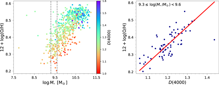
Figure 1. Left panel: global MZ relation color-coded with D(4000). Given M⋆, galaxies with larger metallicity tend to have larger D(4000) (i.e., older stellar ages). Right panel: scatter plot gas metallicity vs. strength of the 4000 Å break for the galaxies in the mass bin  , which is marked with dashed lines in the left panel. The red solid line represents the ODR fitting of the data points.
Download figure:
Standard image High-resolution imageTable 1. Global and Local Parameters of the Individual Galaxies
| Galaxy ID |

| Zg | D(4000) |
 Slope Slope | Age⋆–Zg Slope |
|---|---|---|---|---|---|
| (M⊙) | (dex) | (Original) | (Residual) | ||
| (1) | (2) | (3) | (4) | (5) | (6) |
| 7443-12703 | 11.07 | 8.47 | 1.16 | −0.07 ± 0.04 | +0.09 ± 0.03 |
| 7443-9101 | 10.68 | 8.48 | 1.16 | +0.47 ± 0.09 | +0.52 ± 0.09 |
| 7495-12704 | 10.72 | 8.58 | 1.33 | −0.23 ± 0.07 | −0.24 ± 0.03 |
| 7495-9101 | 9.18 | 8.31 | 1.16 | +2.0 ± 0.4 | +1.7 ± 0.3 |
| 7815-12701 | 9.43 | 8.33 | 1.19 | +0.38 ± 0.15 | +0.34 ± 0.12 |
| 7815-12702 | 9.65 | 8.37 | 1.26 | +1.1 ± 0.3 | −4.9 ± 0.3 |
| 7815-12704 | 10.87 | 8.54 | 1.42 | −0.14 ± 0.07 | −0.23 ± 0.06 |
| 7815-9101 | 10.21 | 8.51 | 1.27 | +1.2 ± 0.2 | −0.13 ± 0.09 |
| 7815-9102 | 9.66 | 8.38 | 1.19 | +0.4 ± 0.6 | +0.17 ± 0.13 |
| 7957-12702 | 10.50 | 8.45 | 1.23 | +1.03 ± 0.09 | +0.17 ± 0.04 |
| 7957-12704 | 10.16 | 8.45 | 1.25 | +0.60 ± 0.11 | +0.19 ± 0.05 |
| 7957-9101 | 9.77 | 8.38 | 1.18 | +0.9 ± 0.2 | +0.13 ± 0.13 |
| 7957-9102 | 10.30 | 8.51 | 1.20 | +1.70 ± 0.17 | +0.19 ± 0.04 |
| 7958-12701 | 9.61 | 8.30 | 1.12 | +0.3 ± 0.2 | +0.11 ± 0.08 |
| 7958-12703 | 10.18 | 8.48 | 1.25 | +0.30 ± 0.14 | −0.01 ± 0.11 |
| 7958-12705 | 9.82 | 8.32 | 1.21 | +0.47 ± 0.12 | +0.28 ± 0.07 |
| 7960-12701 | 11.01 | 8.56 | 1.26 | −0.24 ± 0.07 | −0.35 ± 0.04 |
| 7960-12703 | 10.24 | 8.52 | 1.29 | +1.7 ± 0.2 | +0.14 ± 0.07 |
| 7960-12704 | 10.40 | 8.44 | 1.20 | +1.82 ± 0.14 | +0.79 ± 0.07 |
| 7960-12705 | 10.51 | 8.57 | 1.33 | −0.19 ± 0.17 | +0.02 ± 0.04 |
| 7962-12701 | 9.96 | 8.46 | 1.17 | +1.1 ± 0.2 | +0.17 ± 0.08 |
| 7962-12702 | 10.38 | 8.45 | 1.21 | +1.7 ± 0.2 | +0.38 ± 0.07 |
| 7962-12703 | 11.12 | 8.53 | 1.42 | −0.33 ± 0.06 | −0.11 ± 0.04 |
| 7962-12704 | 10.16 | 8.52 | 1.28 | −0.38 ± 0.12 | −0.05 ± 0.03 |
| 7964-12701 | 9.51 | 8.36 | 1.27 | +0.58 ± 0.18 | +0.60 ± 0.12 |
| 7968-12702 | 10.44 | 8.52 | 1.30 | +0.38 ± 0.09 | +0.17 ± 0.05 |
| 7972-12703 | 10.36 | 8.53 | 1.34 | −0.28 ± 0.08 | −0.11 ± 0.06 |
| 7972-12704 | 10.10 | 8.51 | 1.31 | +1.2 ± 0.2 | +0.08 ± 0.08 |
| 7975-12705 | 9.77 | 8.31 | 1.17 | +1.05 ± 0.18 | +0.20 ± 0.14 |
| 7975-9102 | 10.31 | 8.49 | 1.27 | +0.57 ± 0.12 | +0.11 ± 0.06 |
| 7977-9101 | 11.23 | 8.55 | 1.18 | −0.11 ± 0.12 | −0.05 ± 0.07 |
| 7990-12701 | 10.19 | 8.54 | 1.29 | +0.20 ± 0.17 | −0.40 ± 0.10 |
| 7990-12704 | 10.51 | 8.53 | 1.39 | −0.13 ± 0.09 | −0.22 ± 0.07 |
| 7990-9101 | 10.20 | 8.55 | 1.38 | −0.3 ± 0.2 | −0.44 ± 0.15 |
| 7991-12701 | 10.65 | 8.48 | 1.16 | +0.93 ± 0.11 | +0.29 ± 0.04 |
| 7991-12704 | 9.83 | 8.50 | 1.25 | +0.8 ± 0.2 | +0.23 ± 0.06 |
| 7991-9101 | 10.14 | 8.54 | 1.31 | +0.09 ± 0.10 | −0.25 ± 0.06 |
| 7992-9101 | 9.44 | 8.30 | 1.21 | +0.6 ± 0.3 | +1.89 ± 0.19 |
Note. From left to right, the columns correspond to (1) galaxy ID, defined as the [plate]-[ifudesign] of the MaNGA observations; (2) galaxy stellar mass; (3) gas-phase oxygen abundance; (4) 4000 Å break index; (5) slope of the original local Age⋆–Zg relation; and (6) slope of the residual local Age⋆–Zg relation.
Only a portion of this table is shown here to demonstrate its form and content. A machine-readable version of the full table is available.
Download table as: DataTypeset image
5. The Local Age⋆–Zg Correlation
To our knowledge, no previous investigation of the local Age⋆–Zg relation has been carried out so far. For the first time, we seek a such a correlation and its connection with the galaxy-integrated trend linking both parameters.
For this local approach, one has to bear in mind that the 2D maps of all stellar properties derived with Pipe3D, including D(4000), present a spatial binning beyond the spaxel size, which was adopted to increase the S/N of the spectra so as to obtain an accurate estimation of the stellar contribution. The typical size of the bins ranges between 2 and 5 spaxels in most cases, with a few larger ones in the outer regions of the galaxies (for more information on this spatial binning and its implementation in MaNGA, see Sánchez et al. 2019a). However, gas properties such as Zg are estimated in every single spaxel. In order to reconcile the two different scales, all of the star-forming spaxels belonging to the same bin are considered as a single data point, with its Zg defined as the average value within the bin and its D(4000) as the value derived by Pipe3D from the fitting of the coadded spectra within the bin.
In order to describe the local relation between these quantities, we follow two different approaches: (1) to include their radial decline when moving from the inner to the outermost parts of galaxy disks and (2) to describe their local variations once the overall radial profiles have been removed. Hereafter, we will refer to them as original and residual local relations, respectively. For the original relation, we examine for each galaxy the scatter plot D(4000) versus Zg for all star-forming bins. For the residual relation, we analyze the correlation between the residuals. These residuals are obtained by subtracting the azimuthally averaged radial Zg and D(4000) distributions from the 2D maps. These averaged values are measured in elliptical annuli centered at each data point, taking into account the position angle and ellipticity of the galaxies to correct for inclination. The width of the annuli is 2'', which is comparable to the spatial resolution of the data (see Section 2.1).
Figure 2 shows scatter plots representing the original (middle) and residual (right) Age⋆–Zg local relations derived for one typical galaxy of the sample, 7960-12704. The average error of the analyzed star-forming regions is displayed in the top left corner of each panel. We note that the calibration error of the O3N2 metallicity indicator (0.08 dex) is not included. For the particular galaxy shown in Figure 2, positive correlations can be observed between both the original (middle panel) and residual (right panel) variations of Zg and D(4000). In order to quantify the correlations, we perform an ODR fitting to the data points enclosed within the 80% level density contour (i.e., the contour that encircles 80% of the total number of data points; red dashed line). The error in the linear fit (brown shaded area) is estimated by bootstrapping. We show the standard deviation of the slopes in 100 fits inferred from a random resampling of the data with replacement (i.e., each data point can appear multiple times in the sample). The rms error (RMSE) of the fit is 0.033 for the original relation (middle) and 0.028 for the residual relation (right). On average, the galaxies in the sample present a slightly smaller RMSE, with median values of 0.024 and 0.018, respectively. This scatter is similar to the one found for the local relation between SFR and Zg described in SM19.
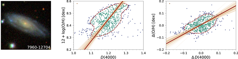
Figure 2. Scatter plots representing the original (middle panel) and residual (right panel) local relations between the gas metallicity and the 4000 Å break for one typical galaxy of the sample, 7960-12704. Its SDSS color image is shown in the left panel. The red solid lines correspond to an ODR fitting to the data points enclosed within the 80% density contour indicated by the red dashed lines, and the shaded areas show the error region estimated by bootstrapping (see main text). The error bars in the top left corner of the panels correspond to the average error of all analyzed spaxels. Note that the calibration error associated with the use of the O3N2 metallicity indicator is not included.
Download figure:
Standard image High-resolution imageThe local relations between D(4000) and Zg are derived for all galaxies in the sample, and the resulting slopes of the linear fits, together with their corresponding errors, are listed in Table 1. In order to have sufficient statistics for the fits, 68 galaxies containing less than 30 data points (i.e., bins) are discarded from the analysis. We find that 65% of the remaining 668 galaxies display a positive correlation (i.e., positive slope) within the error bars, 20% of them present an anticorrelation (i.e., negative slope), and the remaining 15% are compatible with the absence of correlation (i.e., zero slope). When considering the residuals ΔD(4000) and ΔZg , 47% (31%) of the galaxies show positive (negative) correlation, with 22% of the sample showing a lack of correlation within the observational errors.
To investigate how the local relation between D(4000) and Zg
depends on the galaxy mass, Figure 3 shows the slope of each galaxy as a function of the stellar mass for the original (left) and residual (right) relations. Overall, we can see that lower-mass galaxies present a local correlation between the gas metallicity and the stellar age with a larger slope than more massive galaxies, where the correlation tends to disappear. This behavior is shown by the red solid lines, which represent the variation of the mean slope with M⋆. In the case of the residual local relation (right panel in Figure 3), the derived slopes are a bit smaller but differ significantly from zero. The residual local relation exhibits also the same tendency shown by the original local relation (left panel in Figure 3) of the least massive galaxies presenting the largest slopes. Moreover, in this case, the relation reverses at  , with more massive galaxies presenting an anticorrelation between the residuals ΔD(4000) and ΔZg
; that is, older is less metallic.
, with more massive galaxies presenting an anticorrelation between the residuals ΔD(4000) and ΔZg
; that is, older is less metallic.
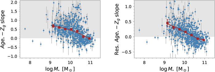
Figure 3. Variation with galaxy mass of the slope of the original (left panel) and residual (i.e., after removing the radial gradients of both parameters; right panel) Age⋆–Zg
local relations. The red squares represent the mean slope in seven stellar mass bins, with the error bars indicating the error given by  (σbin is the standard deviation of the slopes in each bin, and Nbin is the number of galaxies within). In most cases, the error bars are smaller than the marker size. The average values (red squares) were fitted with a third-order polynomial (red solid lines).
Download figure:
Standard image High-resolution image6. Linking the Global and Local Trends
As explained in Section 1, SA19 derived an analytical formulation to draw global laws from local ones. As an example, they showed how the global FMR emerges from the local correlation between SFR surface density and Zg found by SM19. In this section, we study the correspondence between the local and global trends for the Zg versus D(4000) relation described in Sections 4 and 5.
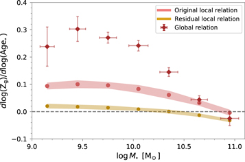
Figure 4 shows the comparison of the slopes inferred from the global and local relations between Zg and D(4000) at each M⋆. For the global trend (diamonds), the error bars represent the standard deviation of the slopes derived in each mass bin from the integrated Zg and D(4000) values in 100 fits inferred by bootstrapping. For the local trend, we represent both the original relation (pink markers) and the residual one (yellow markers). In this case, the shaded areas denote the error of the mean slope of the individual galaxies within each mass bin, as indicated by the error bars in Figure 3. We can see that the three relations show the same trend, that is, a decreasing slope with increasing galaxy mass. In spite of the similarity in the tendency, the relations do not agree quantitatively; the global relation has slopes larger than the local ones in the low-mass regime, with the residual local relation presenting the values closest to zero. The explanation for the qualitative agreement and the seeming quantitative discrepancy is discussed in Section 7.
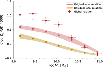
Figure 4. Comparison of the slopes inferred from the local and global Age⋆–Zg relations as function of M⋆. The pink and yellow markers represent the mean slopes for the different mass bins obtained from spatially resolved data for the original and residual local relations, respectively. The errors of these quantities are denoted by the shaded areas. The diamonds show the slopes derived from galaxy-integrated values using exactly the same MaNGA sample, with the error bars indicating the standard deviation in 100 fits inferred by bootstrapping (see main text).
Download figure:
Standard image High-resolution image7. Discussion and Conclusions
The search for relations between integrated physical properties in galaxies has been widely addressed in the literature. With the advent of IFS, the availability of spectra providing spatially resolved information for large samples of galaxies has shown that many of these global trends emerge from local correlations. An example is the FMR, which is claimed to arise from the local anticorrelation between surface density SFR and Zg found by SM19 (see also Sánchez Almeida et al. 2018, for previous findings on dwarf galaxies). The mathematical correspondence between both relations described by SA19 predicts that the same global–local equivalence should hold for other parameters.
In this study, we analyze IFS data for a sample of 736 star-forming disk galaxies from the MaNGA survey. The aims of this analysis are to (i) explore the existence of a local counterpart for a specific global relation, (ii) investigate how the global and local trends compare with each other, and (iii) assess the validity of the prediction given in SA19 for the mathematical equivalence between the analyzed global law and the corresponding local correlation.
The examined relation links the gas metallicity and the stellar age. At a fixed stellar mass, galaxies with younger stellar populations (characterized by larger D(4000) values) present lower Zg
(Lian et al. 2015). This trend is explained as a natural result of passive evolution: galaxies with older stellar populations experience a stronger metal enrichment process and thus exhibit larger gas metallicities. It may also be due to recent metal-poor gas accretion, which simultaneously decreases Zg
and triggers star formation, thus decreasing the mean light-weighted age of the stellar population. Which of the two processes dominate is expected to be a function of M⋆. Dividing the sample into seven mass bins (from 9.0 to 11.1  ), we systematically find a clear positive correlation between global Zg
(expressed as the oxygen abundance measured with the O3N2 indicator) and D(4000), in agreement with Lian et al. (2015). The slope of the correlation decreases when increasing the mass of the bin and becomes zero at about
), we systematically find a clear positive correlation between global Zg
(expressed as the oxygen abundance measured with the O3N2 indicator) and D(4000), in agreement with Lian et al. (2015). The slope of the correlation decreases when increasing the mass of the bin and becomes zero at about  .
.
We characterize the local relation between Zg
and D(4000) within each galaxy by the slope of an ODR fitting to the scatter plot  versus D(4000) after filtering out extreme values (this is called the original local relation). For the 668 galaxies with reliable fits, we find that 65% present a positive correlation, 20% present a negative correlation, and 15% are compatible within the errors with no correlation between Zg
and D(4000). The positive correlation observed for most galaxies is expected as a consequence of the negative radial gradients found for both the gas metallicity (e.g., Sánchez et al. 2014; Ho et al. 2015; Sánchez-Menguiano et al. 2016; Belfiore et al. 2017) and the stellar age (e.g., Sánchez-Blázquez et al. 2014; González Delgado et al. 2015; Goddard et al. 2017; Ruiz-Lara et al. 2017), which are explained in the framework of an inside-out formation of the galaxy disks (Prantzos & Boissier 2000). The presence of deviations from these radial declines for both parameters (e.g., Ruiz-Lara et al. 2016; Sánchez-Menguiano et al. 2018) might correspond to the cases where a negative or lack of correlation between Zg
and D(4000) has been reported. However, this cannot be the full explanation, since the correlations remain when the radial variations are removed. Moreover, there is a systematic change of the slope with galaxy stellar mass, positive at low mass and negative in the high-mass end.
versus D(4000) after filtering out extreme values (this is called the original local relation). For the 668 galaxies with reliable fits, we find that 65% present a positive correlation, 20% present a negative correlation, and 15% are compatible within the errors with no correlation between Zg
and D(4000). The positive correlation observed for most galaxies is expected as a consequence of the negative radial gradients found for both the gas metallicity (e.g., Sánchez et al. 2014; Ho et al. 2015; Sánchez-Menguiano et al. 2016; Belfiore et al. 2017) and the stellar age (e.g., Sánchez-Blázquez et al. 2014; González Delgado et al. 2015; Goddard et al. 2017; Ruiz-Lara et al. 2017), which are explained in the framework of an inside-out formation of the galaxy disks (Prantzos & Boissier 2000). The presence of deviations from these radial declines for both parameters (e.g., Ruiz-Lara et al. 2016; Sánchez-Menguiano et al. 2018) might correspond to the cases where a negative or lack of correlation between Zg
and D(4000) has been reported. However, this cannot be the full explanation, since the correlations remain when the radial variations are removed. Moreover, there is a systematic change of the slope with galaxy stellar mass, positive at low mass and negative in the high-mass end.
We also study the local relation between the residual ΔZg and ΔD(4000) for all star-forming regions obtained after removing the radial gradients (this is called the residual local relation). Deriving the slope of this correlation for the galaxy sample, we find that 47% exhibit positive correlation, 31% negative correlation, and the remaining 22% lack of correlation between ΔZg and ΔD(4000). These results confirm that, similar to the global trend, older star-forming regions generally exhibit larger gas metallicities compared to younger regions within the same galaxy.
For both the original and residual Age⋆–Zg
local relations, we find that the slope depends on M⋆, so that less massive galaxies are characterized by larger slopes than more massive systems. In the first case, the correlation disappears at about  , whereas this happens at
  for the residual local relation, reversing the relation for galaxies more massive than that. Considering that the stellar age provides rough estimates for the shape of the star formation history (SFH) of a galaxy, this indicates that the SFH of older and more massive regions presents little variation, on average. However, at low mass, we find a wide range of SFHs (and chemical enrichment; e.g., Ibarra-Medel et al. 2019).
The trend of the slope of the local relations with galaxy mass resembles that of the global law. As we discuss in Section 1, every global correlation should come together with a local counterpart, with the slopes of the global and local laws expected to be the same. However, we find the local correlations to have systematically smaller slopes than the global correlation. This is clear in the relation between excess of metallicity and excess of age (Figure 4). The largest discrepancies are found for low-mass galaxies, where the slopes of the residual local relation are as low as half the slope of the global relation (although the error bars associated with the global slopes are also larger in this mass range, which could account for part of the discrepancies). A much better agreement is found for high-mass galaxies, where the differences are reduced by more than half. These differences do not disappear when deriving stellar ages from SSP fitting (see Appendix B). Indeed, although similar trends are observed for the mass dependence of both the global and local relations, the reported slopes of the relations are significantly lower than when using D(4000). This is especially noticeable for the residual local relation, where the percentage of slopes compatible with zero has significantly increased (from 22% to 45%), making the differences between the global and local relations more pronounced. However, we think that the uncertainties involved in the inversion method and the complex modeling of the stellar populations applied to spatially resolved IFS data (e.g., Cid Fernandes et al. 2014; Sánchez et al. 2016a; Bittner et al. 2019) might be partially responsible for these larger discrepancies. As we argue below, the clearer Age⋆–Zg relations reported when using D(4000) do not result from the possible influence of other physical parameters on D(4000) but describe a true relation between gas metallicity and stellar age.
The derivation of the gas metallicity also involves an important number of systematics and sources of uncertainties, with well-known discrepancies between the use of different strong-line calibrators (e.g., Kewley & Ellison 2008; López-Sánchez et al. 2012). In this regard, to assess whether the choice of the gas metallicity indicator affects the quantitative disagreement between the local and global laws, we alternatively derive the oxygen abundance by making use of the theoretical calibrator HII-CHI-MISTRY (Pérez-Montero 2014) based on photoionization models from CLOUDY (Ferland et al. 2013). The new comparison of the slopes inferred from the local and global  relations as a function of M⋆ is shown in Figure 5. Consistent with the use of the O3N2 indicator, we obtain the same trend for both local and global relations of decreasing the slope when increasing the galaxy mass, with the majority of the galaxies (except the most massive ones) presenting a positive correlation between Zg
and D(4000). In spite of the local relations displaying larger dispersions, with HII-CHI-MISTRY, we find that the quantitative agreement between the local and global relations is significantly better, with a reduction in the slope differences up to 60%. However, the differences are still noticeable.
relations as a function of M⋆ is shown in Figure 5. Consistent with the use of the O3N2 indicator, we obtain the same trend for both local and global relations of decreasing the slope when increasing the galaxy mass, with the majority of the galaxies (except the most massive ones) presenting a positive correlation between Zg
and D(4000). In spite of the local relations displaying larger dispersions, with HII-CHI-MISTRY, we find that the quantitative agreement between the local and global relations is significantly better, with a reduction in the slope differences up to 60%. However, the differences are still noticeable.
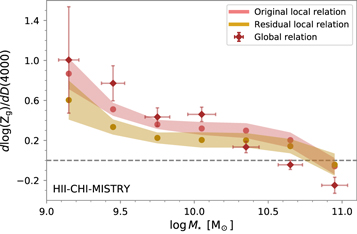
Figure 5. Comparison of the slopes inferred from the local and global Age⋆–Zg relations as function of M⋆. Here Zg is determined using the HII-CHI-MISTRY calibration. See caption of Figure 4 for more details.
Download figure:
Standard image High-resolution imageThe question arises as to whether the observed differences between the global and local relations invalidate the argument that the global correlation arises from the spatial integration of the local correlation. It does not. As we show in Appendix C, the effect of random noise easily explains the difference. The error in determining stellar ages is large. Even if D(4000) is well determined, it is only a proxy for stellar age with large uncertainty (e.g., Sánchez Almeida et al. 2012). As soon as the errors are comparable with the range of abscissae, the slope inferred from a least-squares fitting systematically underestimates the true slope. The fact that errors in spatially resolved data are larger than integrating over a galaxy naturally explains why local slopes are systematically smaller. A factor of 2 drop, consistent with the observations (Figure 4), is easy to account for (see demonstration in Appendix C).
In this study, we show the existence of both a local (spatially resolved) and a global (galaxy-integrated) relation between Zg and D(4000), which we interpret as a true relation between gas metallicity and stellar age. However, there is evidence of the influence of other physical parameters on D(4000) that might affect this interpretation. One explored parameter is dust attenuation. Usually, D(4000) is considered robust against dust-induced reddening, since it is a differential measure with a relatively small wavelength separation between bands. Therefore, dust is not expected to significantly influence the relation observed between Zg and D(4000), although residual effects might play a role (MacArthur 2005). We explore the impact of dust by investigating the shape of the local relation between dust attenuation (measured using AV ) and gas metallicity. We find that the majority of galaxies exhibit negative or close-to-zero slopes, in contrast to the positive slopes of the relation between Zg and D(4000), suggesting, therefore, that the effect of dust, if it exists, is minor. This is also supported by the observed trend for the dependence of the slope with the galaxy mass, with the slope of the AV –Zg relation increasing with galaxy mass, while in the case of the Age⋆–Zg relation, the slope decreases with mass. Another relevant parameter to investigate is the stellar metallicity. One could think that the existence of the Age⋆–Zg relation might be partly induced by the secondary dependence of D(4000) with stellar metallicity. However, we believe that this is not the case, or at least the effect of the stellar metallicity is minor. As shown by Kauffmann et al. (2003), the dependence of D(4000) on stellar metallicity is stronger for older stellar ages, therefore D(4000) is almost insensitive to it for mean ages lower than ∼1 Gyr, corresponding to D(4000) < 1.4–1.5 (∼97% of the data points fall within this range). If the stellar metallicity is responsible for the observed relations, the slope of the relations should increase with the galaxy mass, which is the opposite of the observed behavior, in which the relations disappear for more massive systems. In conclusion, all of this reasoning reinforces that the described relation between Zg and D(4000) corresponds to a true relation between gas metallicity and stellar age. Since, as argued above, the strength of the 4000 Å break is a measure of the relative contribution of young hot stars, it gives an estimate of the specific SFR of the galaxy (e.g., Bruzual 1983). For this reason, the correlation between stellar age (or D(4000)) and gas metallicity is probably directly related to the anticorrelation between Zg and SFR found by SM19, as both of them have the same physical origin.
In summary, this work shows for the first time the existence of a positive linear correlation between D(4000) (used as an indicator of stellar age) and Zg at local scales (before and after correcting for radial trends), with a slope that decreases with increasing the galaxy stellar mass. The same trend is also reported for the global (integrated) values, confirming previous studies. We find a discrepancy in the slopes, with the local relations presenting systematically smaller values. The uncertainty in the analyzed parameters can account for this difference, making the slope inferred from a least-squares fitting systematically lower than the true value. Therefore, this result suggests that the observed global relation between the stellar age and the gas metallicity emerges from the spatial integration of their local correlation. The extension of this study to other global scaling relations and the search for their corresponding local counterparts can provide important information to constrain numerical simulations so to understand how galaxies form and evolve.
We thank the anonymous referee for suggestions that allowed us to improve the paper. Thanks are also due to Tomás Ruiz-Lara for comments on the original manuscript. This work has been partly funded by the Spanish Ministry of Economy and Competitiveness (MINECO), projects AYA2012-31935 and AYA2016-79724-C4-2-P (ESTALLIDOS). S.F.S. is grateful for the support of CONACYT grants CB-285080 and FC-2016-01-1916 and funding from the PAPIIT-DGAPA-IN100519 (UNAM) project.
This project makes use of the MaNGA-Pipe3D data products. We thank the IA-UNAM MaNGA team for creating it and the CONACYT-180125 project for supporting them.
Funding for the Sloan Digital Sky Survey IV has been provided by the Alfred P. Sloan Foundation, the U.S. Department of Energy Office of Science, and the Participating Institutions. The SDSS acknowledges support and resources from the Center for High-Performance Computing at the University of Utah. The SDSS website is www.sdss.org.
The SDSS is managed by the Astrophysical Research Consortium for the Participating Institutions of the SDSS Collaboration, including the Brazilian Participation Group, the Carnegie Institution for Science, Carnegie Mellon University, the Chilean Participation Group, the French Participation Group, Harvard-Smithsonian Center for Astrophysics, Instituto de Astrofísica de Canarias, The Johns Hopkins University, Kavli Institute for the Physics and Mathematics of the Universe (IPMU)/University of Tokyo, the Korean Participation Group, Lawrence Berkeley National Laboratory, Leibniz Institut für Astrophysik Potsdam (AIP), Max-Planck-Institut für Astronomie (MPIA Heidelberg), Max-Planck-Institut für Astrophysik (MPA Garching), Max-Planck-Institut für Extraterrestrische Physik (MPE), National Astronomical Observatories of China, New Mexico State University, New York University, the University of Notre Dame, Observatório Nacional/MCTI, The Ohio State University, Pennsylvania State University, Shanghai Astronomical Observatory, the United Kingdom Participation Group, Universidad Nacional Autónoma de México, the University of Arizona, the University of Colorado Boulder, the University of Oxford, the University of Portsmouth, the University of Utah, the University of Virginia, the University of Washington, the University of Wisconsin, Vanderbilt University, and Yale University.
Software: astropy (Astropy Collaboration et al. 2013, 2018), Matplotlib (Hunter 2007).
Appendix A: Testing the Robustness of the Results
In this appendix, we describe several tests performed to assess whether the reported results might be affected by different criteria applied along the study. All tests show that the sample selection and analysis are robust, and the results are not contingent upon any of the examined factors.
In the first place, due to the wide range of redshifts covered by the MaNGA mother sample, the physical spatial resolution of the data can vary significantly. This effect could bias the results, in that the galaxies with no observed local correlations could be due to the low spatial resolution of the data and not because of a physical cause. In order to prevent this potential bias, the original sample was restricted to galaxies with z < 0.05 and observed with the two largest FoVs (275 and 213). In spite of this, here we further investigate the effect of the spatial resolution on the results by removing from the sample those objects with Re below three times the seeing FWHM. The remaining 456 galaxies cover the same parameter space for the analyzed local relations as the whole sample, showing no bias of the measured slopes related to spatial resolution. Although with a much smaller number statistics, restricting to galaxies with Re > 4 FWHM produces the same result.
Along the same lines, the MaNGA data show a certain degree of oversampling due to the small size of the spaxels (05) in comparison with the final spatial resolution (FWHM ≃ 25). This can induce some correlation in the data points of the local relations, which, in the case of galaxies with a low number of points, might affect their determination. In this regard, we have investigated how the derived slopes are influenced by the number of points involved in their computation. We increased the threshold in the number of points requested to perform the linear fits from 30 to 100, with no significant biases in the coverage of the parameter space of the two analyzed local relations. Therefore, the cases where no correlation is found do not seem to be associated with a possible oversampling of the data.
Another factor we have explored is the spatial coverage of the galaxies. As mentioned in Section 2.1, the coverage of the MaNGA galaxies is not homogeneous, but some systems are observed up to 2.5–3 Re , whereas others are observed just up to 1–1.5 Re . Thus, our results might overweight the centers of the galaxies so that the observed behavior might depend on the fraction of the galaxy that is covered. To address this issue, we removed from the sample those galaxies for which the FoV covers less than 2 Re . Although the number of analyzed objects is reduced to 224, we observe a similar distribution of slopes for the local relations, and also the same trend of the slopes decreasing with increasing the stellar mass remains. Therefore, the differences in the spatial coverage of the analyzed sample do not seem to significantly affect the results either.
Additional tests have been performed to assess the effect of including mergers in the sample or galaxies that are too inclined to properly map the spatial variations across the disks. For the first case, we make use of the attribute P_merg, available in the MaNGA Deep Learning Morphology Value Added Catalog (MDLM-VAC) published in Fischer et al. (2019; also used for the morphological classification of the sample; see Section 2.2). This parameter measures the probability of a merger signature (or projected pair). Removing from the sample 84 galaxies with P_merg > 0.8, we find no significant differences in the coverage of the parameter space for the local relations. Lastly, restricting to very face-on galaxies (i < 45°) produces no noticeable bias in the results.
For the spaxel selection, as explained in Section 3, we impose a lower limit of S/N = 3 in all of the emission lines involved in the derivation of the oxygen abundances, namely, Hβ, [O iii] λ5007, Hα, and [N ii] λ6584. This restrictive limit preferentially excludes spaxels with weak emission, which may bias the local relations somehow. In order to investigate this effect, we compare the slopes of the local relations of 100 randomly selected galaxies using an S/N threshold of 1 and 3. We obtain very similar values in all cases, and a representation of one against the other shows nearly one-to-one relations (slope of 0.96 for the original relation and 1.01 for the residual relation) with very high correlation coefficients (0.94 and 0.92, respectively). This indicates that spaxels with S/Ns below and above 3 present similar distributions in the D(4000) − Zg parameter space; hence, the values of the slopes hardly change.
In order to describe the global relation for D(4000) and Zg , we use the average values of all analyzed star-forming regions as characteristic of the population of the entire galaxy (this is explained in Section 3.1). However, as these properties are not constant across galaxies but present a radial decrease, their estimation might be affected by the radial extension of the galaxy covered with MaNGA data. We explored the impact of these aperture effects on the global relation (their influence on the local relation was already examined). Instead of using the average D(4000) and Zg of the analyzed star-forming regions, we made use of the characteristic values at 1 Re . The resulting global Age⋆–Zg relation is very similar to that shown in Figure 4, with comparable slopes in all mass ranges.
Finally, for the characterization of the local Age⋆–Zg relations, we perform an ODR fitting to the data points of each individual galaxy enclosed within the 80% level density contour in order to avoid outliers influencing the fits (see Section 5). We have also tested how the use of this cut might affect the analysis. The slopes derived with and without the mentioned cut are in very good agreement with each other for both the original and residual relations. We obtain tight correlations very close to the one-to-one relation with high correlation coefficients (∼0.8). Furthermore, the trend of the slope of the local relations with galaxy mass show very similar behaviors to those described in Figure 3, with almost imperceptible differences, concluding that the use of the cut does not change the overall results.
Appendix B: The Age⋆–Zg Relation from the Stellar Continuum Fitting
As a result of the stellar continuum fit, Pipe3D provides 2D luminosity-weighted (LW) stellar age maps from the individual weights of the combined SSPs (see Section 3). However, as explained in Section 4, we prefer to use D(4000) as a proxy for the age of the stars, avoiding the uncertainties involved in the inversion method and the complex modeling of the stellar populations applied to spatially resolved IFS data (e.g., Cid Fernandes et al. 2014; Sánchez et al. 2016a; Bittner et al. 2019). Nevertheless, for the sake of comprehensiveness, this appendix shows the comparison of the corresponding local and global  relations using the 2D LW stellar age maps provided by Pipe3D.
The local relations between Age⋆ and Zg are derived for all galaxies in the sample. We find a positive (negative) slope for 58% (15%) of the galaxies. The remaining 27% are compatible with absence of correlation (i.e., zero slope). When considering the variations of the residuals ΔAge⋆ and ΔZg , just 27% (28%) of the galaxies show a positive (negative) correlation, with 45% of the sample showing a lack of correlation within the observational errors. The high presence of no correlations is probably due, as mentioned in Appendix C, to the typical uncertainty associated with age determinations from spectral fitting, since the percentage of slopes compatible with zero is significantly smaller (22%) when using D(4000).
Figure 6 shows the slope of the original (top) and residual (bottom) local relations as a function of galaxy mass (see Section 5 for details on the layout of the figure). For the original relation (top panel), we see that lower-mass galaxies present a larger slope than more massive galaxies, where the slope tends to zero and the correlation disappears. In the case of the residual local relation (bottom panel), the slopes are very small for most galaxies, although again, the least massive galaxies tend to display the largest slopes. Similarly to D(4000), the relation reverses at  , with more massive galaxies showing an anticorrelation between the variations of the residuals ΔAge⋆ and ΔZg
.
, with more massive galaxies showing an anticorrelation between the variations of the residuals ΔAge⋆ and ΔZg
.
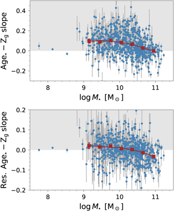
Figure 6. Slope of the Age⋆–Zg local relations as function of M⋆ (original, top; residual, bottom). Age⋆ is derived from the stellar continuum fit. See caption of Figure 3 for more details.
Download figure:
Standard image High-resolution imageFinally, Figure 7 represents the comparison of the slopes derived from the global and local relations at each M⋆ (see Section 6 for details on the layout of the figure). For the global law, we use the mean LW stellar age value measured for all analyzed bins associated with star formation as characteristic of the population of the entire galaxy (see Section 5 for details on the binning scheme). We can see that, overall, the three relations show the same tendency of decreasing slope with increasing galaxy mass. In spite of the similarity in the tendency, the relations do not agree quantitatively; the global relations reach much more positive slopes than the local ones in the low-mass regime, with the residual local relation presenting the values closest to zero. As we argue in Appendix C, the presence of noise can explain these differences between local and global correlations, as well as the difference in the correlations found when using D(4000) as an age indicator (Section 6).
Figure 7. Comparison of the slope inferred from local and global Age⋆–Zg relations as a function of M⋆. Age⋆ is derived from the stellar continuum fit. See caption of Figure 4 for more details.
Download figure:
Standard image High-resolution image
Appendix C: Random Noise Explains the Difference in Slopes between Local and Global Relations
Suppose that two variables, x and y, are related linearly so that

We observe them in N different points with some error, i.e.,

where xio
and yio
are the ith observation, xi
and yi
follow the law in Equation (C1), and Δxi
and Δyi
are the error in the two observed variables. Here Δxi
and Δyi
are assumed to be random independent variables of mean zero and variance  and
and  , respectively. We try to infer the slope m through the customary least-squares fit, i.e.,

Using Equation (C2) and neglecting all sums expected to average to zero (i.e., those having Δxi , Δyi , yi Δxi , xi Δyi , xi Δxi , and Δxi Δyi ), one ends up with an expression for the least-squares slope mls in terms of the true slope m,

with  defined as

Here rmsx is the typical range of abscissae used in the fit. Thus, as soon as the range of abscissae is comparable to their error (rmsx ∼ σx ), the least-squares-based slope is significantly smaller than the true slope (mls ∼ m/2). As an example, the data points in Figure 2 have σx /rmsx of the order of 0.89 and 0.86 (middle and right panels, respectively). The mean value of the ratio considering 100 randomly selected galaxies is 0.8. Here σx was estimated from the observed points as the standard deviation of the observed D(4000) (or ΔD(4000)) minus the value predicted by the linear fit, and RMXx was estimated as the standard deviation of the D(4000) (or ΔD(4000)) predicted by the linear fit. The fact that the errors are larger in the spatially resolved data than when integrating over a galaxy naturally explains why local slopes are systematically smaller.