


Abstract
HD 219134 is a K3V dwarf star with six reported radial-velocity discovered planets. The two innermost planets b and c show transits, raising the possibility of this system to be the nearest (6.53 pc), brightest (V = 5.57) example of a star with a compact multiple transiting planet system. Ground-based searches for transits of planets beyond b and c are not feasible because of the infrequent transits, long transit duration (∼5 hr), shallow transit depths (<1%), and large transit time uncertainty (∼half a day). We use the space-based telescopes the Arcsecond Space Telescope Enabling Research in Astrophysics (ASTERIA) and the Transiting Exoplanet Survey Satellite (TESS) to search for transits of planets f (P = 22.717 days and  ) and d (P = 46.859 days and
  ). ASTERIA was a technology demonstration CubeSat with an opportunity for science in an extended program. ASTERIA observations of HD 219134 were designed to cover the 3σ transit windows for planets f and d via repeated visits over many months. While TESS has much higher sensitivity and more continuous time coverage than ASTERIA, only the HD 219134 f transit window fell within the TESS survey's observations. Our TESS photometric results definitively rule out planetary transits for HD 219134 f. We do not detect the Neptune-mass HD 219134 d transits and our ASTERIA data are sensitive to planets as small as 3.6 R⊕. We provide TESS updated transit times and periods for HD 219134 b and c, which are designated TOI 1469.01 and 1469.02 respectively.
Export citation and abstract BibTeX RIS
1. Introduction
1.1. The HD 219134 Planetary System
HD 219134 is a bright, nearby K3V star reported to host six radial-velocity discovered exoplanets (Motalebi et al. 2015; Vogt et al. 2015; Johnson et al. 2016; Gillon et al. 2017). The two innermost planets HD 219134 b and c, with periods of 3.1 and 6.8 days respectively, were found to transit with Spitzer (Motalebi et al. 2015; Gillon et al. 2017). For planetary system parameters see Table 1 and Figure 1. HD 219134 is the nearest and brightest star presently known to host transiting planets (6.53 pc, Gaia Collaboration et al. 2018; Stassun et al. 2018; and V = 5.57, Oja 1993), making HD 219134 b and c eminently well suited for follow-up atmospheric characterization. HD 219134, also known as TOI 1469, has a stellar radius of  (Boyajian et al. 2012) and stellar mass of
  (Gillon et al. 2017), with R.A. = 23:13:16.780 and decl. = +57:10:10.05 (J2015.5). For other stellar parameters see the Appendix.

Figure 1. Architecture of the inner HD 219134 planetary system. Four of the six reported planets are shown with their approximate relative sizes. Planets b and c have measured radii based on their transits. The radii of planets d and f are assigned from planets with similar masses. Exterior planets g and h are not shown, because ASTERIA did not obtain measurements during their potential transit windows. Figure adapted from: http://backalleyastronomy.blogspot.com/2017/04/.
Download figure:
Standard image High-resolution imageTable 1. Parameters for HD 219134 Planets b, c, f, and d
| Planet | P (d) | a (au) | M ( ) ) |
R ( ) ) |
e |
|---|---|---|---|---|---|
| b | 3.092926 ± 0.000010 | 0.03876 ± 0.00047 | 4.74 ± 0.19 | 1.602 ± 0.055 | 0 (fixed) |
| c | 6.76458 ± 0.00033 | 0.06530 ± 0.00080 | 4.36 ± 0.22 | 1.511 ± 0.047 | 0.062 ± 0.039 |
| f | 22.717 ± 0.015 | 0.1463 ± 0.0018 | >7.30 ± 0.40 | ⋯ | 0.148 ± 0.047 |
| d | 46.859 ± 0.028 | 0.2370 ± 0.0030 | >16.17 ± 0.64 | ⋯ | 0.138 ± 0.025 |
Note. P is period in days, a is semimajor axis in astronomical units, M⊕ is planet mass in Earth masses, R⊕ is planet radius in Earth radii, and e is orbital eccentricity. Planet masses for f and d are minimum masses, hence the > sign. Planets f and d (and g, not shown) are less firm than planets b and c due to their orbital periods' proximity to the stellar rotation period (45.6 days) or its harmonics (Johnson et al. 2016; Folsom et al. 2018). Data from Gillon et al. (2017). For updated P for planets b and c, see Table 3.
Download table as: ASCIITypeset image
The HD 219143 planetary system has promise to be the nearest, brightest example of a compact multiple-planet transiting system—over 100 times closer and more than 200 times brighter than the canonical Kepler 11 system (Lissauer et al. 2011). Indeed, even with periods as long as 22.717 and 46.859 days for planets f and d respectively, the planets still have a fairly high transit probability owing to the transiting geometry of planets b and c. Assuming coplanarity of planets f and d with planets b and c, the a posterior transit probabilities of planets f and d are 13.1% and 8.1%, respectively (Gillon et al. 2017).
The detections of planets HD 219134 f, d, and g are less firm than planets b and c, owing to the proximity of their orbital periods to the stellar rotation period (45.6 days) or its harmonics (Johnson et al. 2016; Folsom et al. 2018). While it is not unexpected to see a 2:1 period ratio between planets (e.g., Winn & Fabrycky 2015), it is concerning that the periods of planets f, d, and g happen to be at 1/2, 1, and 2 times the stellar rotation period.
A ground-based search for transits of planets HD 219143 f and d is impractical because of the low frequency and long duration of the transits and the ephemeris uncertainty (see parameters in Table 2). The long periods (approximately 23 and 47 days) mean that the number of transit events per observing season is small, making observable transit events from a single ground-based location rare. The combination of the relatively long transit duration (3.8 hr for planet f and 5.6 hr for planet d) with the uncertainty on the predicted transit time (on the order of half a day, longer than the anticipated transit duration itself) means that it is both difficult and unlikely to catch an entire transit from a single ground-based location. Catching only the ingress or egress makes it difficult to be confident in the detection of the flux decrease or increase. The issues are exacerbated by the shallow transits expected to be roughly 0.1% deep. This small transit depth is at or beyond the typical capabilities of 1 m class ground-based telescopes, the telescopes that are commonly being used for this purpose, even under ideal conditions such that the HD 219134 f and d transits are expected to be shallow with amplitude similar to systematic noise signals that are known to plague ground-based light curves. We note that despite a shallow transit depth of 0.13% ± 0.02%, NGTS-4b was discovered with a single 20 cm aperture telescope, enabled by a combined 28 transits for the 1.34 day orbit with a 272 night baseline (West et al. 2019).
Table 2. HD 219134 f and d Midtransit Times and Other Parameters Used in Our Planet Search. Values from Gillon et al. (2017)
| Planet Parameter | Planet f | Planet d |
|---|---|---|
| Transit Duration (hr) | <3.82 ± 0.22 | <5.62 ± 0.17 |
| Transit Depth (ppm) | >236 ± 8 | >358 ± 7 |
| Planet Radius (R⊕) | >1.31 ± 0.02 | >1.61 ± 0.02 |
| Midtransit Time (BJDTDB - 2450000) | 7,716.31 ± 0.50 | 7,726.03 ± 0.63 |
Note. Planet radii lower limits are based on the extreme case of a pure iron planet. For updated T0, see Table 3.
Download table as: ASCIITypeset image
To search for transits of HD 219134 d and f we used two complementary space-based photometric data sets. The data set from the Arcsecond Space Telescope Enabling Research in Astrophysics (ASTERIA; Smith et al. 2018) has targeted observations with extensive coverage of the transit windows, while the data set from the Transiting Exoplanet Survey Satellite (TESS; Ricker et al. 2015) has better photometric precision.
1.2. ASTERIA
ASTERIA was a small space telescope (10 cm × 20 cm ×30 cm, 12 kg, a "6U CubeSat") deployed from the International Space Station in 2017 November into a low-Earth orbit. The spacecraft was operational until 2019 December and re-entered Earth's atmosphere in late 2020 April. ASTERIA's refractive camera had a 6 cm aperture, 85 mm focal length, a bandpass from 500 nm to 900 nm, a plate scale of 15 8 per pixel, and a field of view of 11
 2 x 96.
ASTERIA was a technology demonstration mission to prove precise pointing and detector thermal control are possible in a small package, with an eye toward enabling high photometric precision. ASTERIA successfully met its requirements by achieving the following performance goals: reaching line-of-sight pointing stability of approximately 05 rms over 20-minute observations, pointing repeatability of 1 mas rms from one observation to the next, and focal plane temperature stability better than ±0.01 K over 20-minute observations (Pong 2018; Smith et al. 2018). Developed at the Jet Propulsion Laboratory (JPL) in collaboration with the Massachusetts Institute of Technology (MIT), ASTERIA traces its roots back to the ExoplanetSat mission concept developed by MIT and Draper Laboratory (e.g., Smith et al. 2010; Pong et al. 2010). For details of the ASTERIA development, flight system, ground system, on-orbit operation, and on-orbit performance see Smith et al. (2018) and Knapp et al. (2020).
ASTERIA used a complementary metal-oxide semiconductor (CMOS) array detector instead of the traditional charge-coupled device (CCD) detector. We chose a CMOS detector primarily for its fast read out (20 Hz; necessary for the fine pointing control algorithm), its ability to operate at room temperature, and its relative insensitivity to radiation damage. CMOS detectors can be operated at room temperature, as they generate ultra-low dark current (20 e-/pixel/s) compared to 250–500 e-/pixel/s generated by CCDs at the same temperature. Hence, CMOS detectors do not require passive or active cooling systems that would otherwise add significantly to the mass and size of the spacecraft. Despite these distinct advantages, CCDs have traditionally dominated space-based imaging and spectroscopy due to their sensitivity via high quantum efficiency.
ASTERIA was not designed to deliver precise photometry, even though its underlying precise pointing and thermal control are enabling technologies for highly precise photometry. Nonetheless, ASTERIA was able to detect the transit of 55 Cnc e, a planet nearly twice the radius of Earth transiting a Sun-sized star with a transit depth of approximately 400 ppm (Knapp et al. 2020). After completion of its 90 day prime mission, ASTERIA was in part used for opportunistic science, including observations of the bright nearby stars Algol, Alpha Centauri A and B, 55 Cancri, and HD 219134.
1.3. TESS
TESS is an MIT-led, NASA Medium-class Explorer Mission that launched in 2018 April (Ricker et al. 2015). TESS carries four identical, specialized wide-field CCD cameras, each covering 24° x 24° on the sky with a 10 cm aperture, a red bandpass of 600–1000 nm, and plate scale of 21'' per pixel. TESS is in an innovative high-Earth lunar resonance orbit (Gangestad et al. 2013) and a highly inclined, highly elliptical orbit in resonance with the moon, giving TESS a relatively unobstructed, continuous orbit night observations in a thermally stable environment.
During its two-year prime mission, TESS surveyed 70% of the sky, by monitoring each 24° x 96° strip of the sky (called a Sector) for two orbits, or 27.4 days. TESS surveyed the southern ecliptic hemisphere in the first year of its prime mission and will complete the northern ecliptic hemisphere during its second and final year of its prime mission in 2020 June.
TESS is anticipated to find thousands of exoplanets during its prime mission (Sullivan et al. 2015; Barclay et al. 2018; Huang et al. 2018), most with orbital periods less than one month. Although TESS will not be able to discover true Earth analogs (that is, Earth-sized exoplanets in 365 day period orbits about Sun-like stars), TESS will be capable of finding Earth-sized and super-Earth-sized exoplanets (where super-Earths are loosely defined as planets with radii up to 1.7 times Earth's radius) transiting M-dwarf stars, stars that are significantly smaller and cooler than our Sun. One of the TESS Level One mission requirements is to deliver 50 small ( ) planets with measured masses to the community.
During TESS' survey of the sky, TESS naturally monitors many known transiting planet-hosting stars, including HD 219134.
In this paper we proceed with a description of our observations and photometric methods in Section 2, present our transit nondetection results and discussion in Section 3, and conclude with a summary in Section 4.
2. Observations and Methods
2.1. ASTERIA Observations
ASTERIA orbited Earth approximately once every 90 minutes, with orbit night typically lasting between 20 and 35 minutes. ASTERIA only observed during orbit night, therefore observations of HD 219134 were not continuous. Furthermore, because of its small aperture, data from different observing sequences must be phase-folded and binned in order to reach the photometric precision needed to detect shallow transits. ASTERIA's observational constraints (e.g., Sun, Moon, and Earth limb exclusion angles) and operational constraints (e.g., spacecraft related factors) are described in detail in Knapp et al. (2020).
We scheduled ASTERIA observations of HD 219134 (see the Appendix) to target the predicted transit windows of planets f and d (Table 2 with values from Gillon et al. 2017). The transit window predictions take into account uncertainty in the midtransit time T0 and other parameters fit in Gillon et al. (2017). The orbital periods of planets f and d are close to 2:1 (see Table 1), so their predicted transits occur close to one another. The first targeted campaign (so08 through so12, where "so" means science observation) spanned the predicted transit of HD 219134 f (midpoint 2018 March 15) and HD 219134 d (midpoint 2018 March 17). The second campaign (ex11, so18, where "ex" means experimental observation) targeted planet f only (midpoint 2018 April 7). Observations during this campaign were affected by unfavorable geometry between the spacecraft and the star, resulting in short duration observations. The third campaign (so21, so22) targeted the f transit primarily, with some overlap with the beginning of the d transit window. The fourth campaign (so33 through so35) targeted both planets' transit windows (2018 June). Campaign five (2018 July, so37, so38) targeted the transit window of HD 219134 f. The final two campaigns in 2018 August and September (so39 through so48) were focused on covering the full 3σ transit window for planet d, with incidental coverage of planet f transit windows. Other opportunistic observations were carried out when science time was available and spacecraft viewing geometry with HD 219134 was favorable.
For a visual representation of the HD 219134 observing sequences of ASTERIA see Figure 2. For transit coverage of HD 219134 in the form of data density per planet phase see the Appendix.
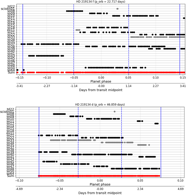
Figure 2. ASTERIA HD 219134 observations. The x-axis shows phase, with phase = 0 corresponding to the predicted transit midpoint. A second horizontal axis shows days from the transit midpoint. The y-axis shows different observing sequences (defined in the Appendix), with each black point corresponding to an orbit night. Gray points indicate observations that were not used in the analysis presented in this paper. The red points and bars at the bottom of the plot represent the union of the black points above. The vertical dashed blue lines show the 1σ transit window as of 2019 March 28; the solid blue bars represent the 3σ transit window for the same date. Top: HD 219134 f. Bottom: HD 219134 d.
Download figure:
Standard image High-resolution image2.2. ASTERIA Data Analysis
Here we provide a summary of our data reduction pipeline, with full details described in Knapp et al. (2020).
2.2.1. ASTERIA CMOS Detector and Calibration Frames
ASTERIA was the first space telescope to attempt science using CMOS detectors. The main difference between CMOS and CCD detectors for precise photometry is that the CMOS readout is parallelized column-wise whereas the pixels of a CCD detector are read out at a single point. For the CMOS detector, each pixel has a different amplifier and each column has a different analog-to-digital converter (ADC). Gains and offsets are therefore column-dependent. The systematics for the ASTERIA CMOS are not as spatially uniform compared to a CCD, because the readout electronics vary column to column.
Due to ASTERIA's status as a technology demonstration mission, there was no requirement or opportunity to characterize the detector in-depth, take calibration data, or validate the photometric performance prior to launch. This affected our data reduction pipeline because we have no ground-based dark frames or flat frames from pre-flight laboratory testing. ASTERIA's camera had no shutter so we could not obtain space-based darks, although dark frames are ultimately not needed for ASTERIA data reduction due to the short 50 ms integration time. ASTERIA did acquire approximated flat frames in space by purposely pointing the telescope in such a way that stray sunlight illuminated the detector. See Knapp et al. (2020) for more details.
Bias was removed from light images column-wise through the use of calibration windows collected contemporaneously with light windows. The calibration window was placed at the bottom edge of the detector where there are both electrically dark pixels (electrically tied to the ground so that photoelectric charge cannot accumulate) and separate optically dark pixels (blocked from light exposure) on the same columns as the light window. We used the electrically dark pixels for the bias correction. See Figure 3, where HD 219134 is centered in window 1 and window 8 is the calibration window.
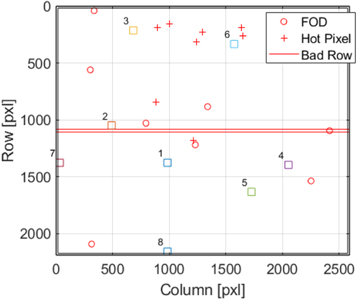
Figure 3. Detector setup for ASTERIA HD 219134 observations. The target star, HD 219134, is centered in window 1. Window 8 served as the calibration window for window 1. The additional windows contain guide stars for ASTERIA's fine pointing algorithm. Known flaws and foreign object debris (FOD) on the detector are also noted.
Download figure:
Standard image High-resolution image2.2.2. ASTERIA Data Reduction
Windowed images from ASTERIA observations were downlinked to the operations center at JPL and then processed into FITS files using custom software. The image data included contemporaneous calibration windows chosen from the edge of the detector (Figure 3). Metadata, including spacecraft housekeeping telemetry, were downlinked separately from the images and then included in the FITS header. Each FITS image contains a 1-minute integration that resulted from the onboard coadding of 1200 individual very short exposure (50 ms) frames. Individual frames were limited to 50 ms in order to support ASTERIA's 20 Hz fine pointing control loop (Pong 2018).
We began the data reduction process by reviewing every frame from the science observations. We manually flagged and discarded frames that were obtained during orbital sunrise or sunset. These frames appeared either at the beginning of an orbit or toward the end of the orbit, and displayed significant background contamination.
After discarding the sunrise/sunset frames, we proceeded to calibrate. We started with bias correction by subtracting the median of the bias column (from the calibration window) from all pixels in the respective column in the science frame. We then selected a few pixels (rows 0–15) in the neighborhood of the target that were devoid of any stellar flux to remove background and/or sky noise. We took the median of the pixels for each column, and subtracted the median value from every pixel in that column. Next, we subtracted the median of the bias rows column by column from every flat frame, and took the median of the reduced flat frame. Lastly, we performed a pixel-by-pixel division of the target star pixels with the reduced flat-frame pixel values. Note that the flat frame used to calibrate HD 219134 data was generated in space using stray light from the Sun to uniformly illuminate the detector as explained earlier (and see Knapp et al. 2020). A representative raw and calibrated image set is shown in Figure 4. The image of the target star is much cleaner than the raw image, although there is still some residual column-dependent noise. For more details on data reduction see Knapp et al. (2020) and Krishnamurthy (2020).
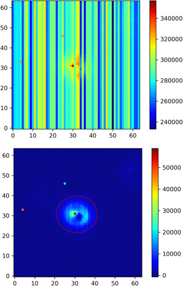
Figure 4. ASTERIA HD 219134 representative raw and calibrated image. The x- and y-axis show the number of pixels for the image, a 64 pixel × 64 pixel window out of a larger 2592 pixel × 2192 pixel CMOS detector. The color bar is light intensity in units of ADU. (Note that nonlinearity becomes important at 30,000 e- and we are operating at ∼4 times below that level.) The defocused star is in the center of the image. Top: the raw image is dominated by column-dependent fixed pattern noise that is a result of gain variations and offsets due to amplifiers and ADC converters respectively. Bottom: calibrated data, after removal of bias and background, and correction for flat-field variations. The donut shape is due to a purposeful defocus design of the ASTERIA camera. Two hot pixels are also visible in the image. The red circle illustrates the aperture we used for photometry.
Download figure:
Standard image High-resolution image2.2.3. ASTERIA Aperture Photometry and Detrending
For aperture photometry, we began by calculating the target x/y position by taking the flux-weighted moments for each pixel in the subarray window. We took the mean centroid position as the target star center, and performed photometric flux extraction using the CircularAperture routine from the photutils (Bradley et al. 2019) python package. We used fixed hard-edge apertures with radii ranging from 5 to 13 pixels. We determined the optimal aperture size by computing the photometric precision for each aperture size given by the rms of the light curve. We obtained an optimal aperture with a radius of 10 pixels based on maximization of the photometric precision (illustrated in Figure 4). We then proceeded to perform photometric flux extraction for all of the HD 219134 data.
For light-curve detrending, we used the Markov Chain Monte Carlo (MCMC) algorithm implementation from Gillon et al. (2012). Inputs to the MCMC were the HD 219134 photometric time series. We explored different functional forms of the baseline model for each light curve. These models could include a linear or quadratic trend with time, a second-order logarithmic ramp (Knutson et al. 2007; Demory et al. 2011) usually included for telescope settling with Spitzer and the Hubble Space Telescope (HST), a polynomial of the (1) centroid position and (2) onboard temperature measured at the lens housing, as well as linear combinations of the point-spread function (PSF) FWHM along the x and y axes. We employed the Bayesian information criterion (BIC; Schwarz 1978) to discriminate between the different baseline models. During our tests, we found that the baseline model resulting in the lower BIC (Schwarz 1978) was a combination of a second-order polynomial of (1) time, (2) x/y centroid position, (3) lens housing temperature, and (4) ASTERIA orbital phase. We note that this baseline model was more complex than the one adopted in Knapp et al. (2020) for 55 Cnc because of the longer photometric sequences used for the search of the longer-period planets in the HD 219134 system.
2.2.4. ASTERIA Transit Injection and Recovery Tests
We performed injection and recovery tests at the 22.717 and 46.859 day periods for HD 219134 f and d respectively, using the allesfitter code (Günther & Daylan 2020), the ellc transit modeling routines (Maxted 2016), and the transit least-square package (Hippke & Heller 2019). We injected different planet sizes at the HD 219134 f and d periods and varied the transit midtimes using a Gaussian distribution matching our calculated transit-timing variation (TTV) amplitudes (see Section 2.5). The period was also allowed to vary in order to generate a T0 span similar to the maximal gradient of the TTV pattern across the ASTERIA observations.
Our transit injection and recovery scheme was thus unusual in the sense that both the periods and transit midtimes were free to vary only within Gaussian priors defined by the transit ephemerides, testing the detection threshold for different radii of HD 219134 f and d.
For both planets f and d we performed injection and recovery tests for radius values ranging between 1.0 and 4.0  , in steps of 0.25 R⊕. ASTERIA observations were limited to 30 minute intervals of night out of a total 90 minute orbit, resulting in noncontinuous observations. The transit injection and recovery does not work as effectively in sparsely sampled data as compared to continuous data, as a large fraction of the transits could fall where data do not exist, hence reducing the detection significance. Because of the low on-target duty cycle, the detection capability for each injected transit is strongly dependent on ASTERIA's resulting window function. Slight changes to the planet's period and/or midtransit ephemerides could then affect the recovery efficiency for both signals. We required a signal-to-noise ratio of 5.
2.3. TESS Observations
TESS observed HD 219134 in camera 3 during Sector 17, from 2019 October 7 to 2019 November 2 and in camera 4 during Sector 24. HD 2190134 has the TESS Input Catalog number TIC 283722336 (Stassun et al. 2018).
The 3σ transit time window of HD 219134 f falls within the TESS observations, based on the ephemeris from Gillon et al. (2017). In contrast, 3σ transit window of HD 219134 d falls outside of the TESS observations.
2.4. TESS Data Analysis
TESS data calibration, reduction, detrending, and light-curve fitting is covered in a large number of papers (e.g., Huang et al. 2018; Vanderburg et al. 2019; Dragomir et al. 2019; Huang et al. 2020). Here we provide a summary of our process.
2.4.1. TESS Data Reduction and Aperture Photometry
We used the calibrated TESS two-minute cadence data produced by the Science Processing Operations Center (SPOC) pipeline based at NASA Ames Research Center (Jenkins 2015; Jenkins et al. 2016).
Because of its considerable brightness (Tmag ∼ 4.6), HD 219134 saturated on the TESS CCDs. We chose to optimize the photometry based on our past experience working with TESS bright stars (Huang et al. 2018; Vanderburg et al. 2019). We re-extracted the photometry using a series of irregular shaped apertures placed on the SPOC-calibrated target pixel stamp. We chose the aperture that minimized the scatter in the out-of-transit portion of the light curve (Figure 5). We next used the SPOC quality flags to eliminate low-quality data points.

Figure 5. TESS custom aperture for HD 219134 on a log scale.
Download figure:
Standard image High-resolution imageFor bright stars, the TESS systematics are mainly due to the pointing jitter of the spacecraft that occur on timescales shorter than the exposure time. We tried to remove such pointing systematics using the standard deviation of quaternion measurements within an exposure (Vanderburg et al. 2019), the first seven SPOC Presearch Data Conditioning (PDC) cotrending basis vectors18 , and also a trigonometric polynomial for longer-term trends. We used a least-squares method to optimize the detrending coefficients by minimizing the out-of-transit scatter of the detrended light curve (for details on the the SPOC PDC see Smith et al. 2012 and Stumpe et al. 2012, 2014).
2.4.2. TESS Transit Injection and Recovery Tests
To search for transits in the TESS data we performed an injection and recovery of transits. We generated transits using BATMAN (Kreidberg 2015) and then injected the transits into the pre-detrended light curve. We investigated the detection rate as a function of planet radii using a grid of planet sizes. The radius grid was  with uniform steps of 0.05 R⊕, and a slightly larger grid using uniform steps of 0.15 R⊕ for larger planetary radii
  .
.
For each planet size, we estimated the detection rate using a binomial distribution from 40 trials. Each trial consisted of injected planets at a given size, using an impact parameter drawn from a uniform distribution between 0 and 1, a randomized T0 with no other restrictions except that T0 falls within the TESS Sector 17 and 24 data, and the period of the planet using the prior constraint from Gillon et al. (2017). Although the T0 and small planet size search parameters are extraneous, we do this to be as exhaustive as possible with our transit search. We then followed the same detrending procedure described above (Section 2.4.1) and ran a box least-square (BLS) search with the period fixed at the best-fitted value from Gillon et al. (2017). For any detected signal, we required the BLS algorithm to recover an epoch within less than half the transit duration of the injected T0, and the signal-to-noise ratio of the recovered transit to be larger than 7.3.
2.5. Transit-timing Variation Methods
We evaluate the range of transit times of planets f and d, considering TTVs of mutual gravitational interactions of the four planets (b, c, f, and d). We used analytic formulae that are accurate to the first order in mass ratios and eccentricity, from Agol & Deck (2016). We verified the validity of the transit times from our analytic approach by using an N-body integrator REBOUND (Rein & Liu 2012), but opted to use the faster analytic approach for our results for efficiency.
We ran a Monte Carlo analysis of the expected TTV amplitudes using a distribution of planetary parameters of the planets in the HD 219134 system to analyze the maximum expected shift in observed time of transit due to TTVs. For this purpose, we used the median values and credible intervals from the global MCMC fit of results from Gillon et al. (2017) to reconstruct Gaussian posteriors for the orbital parameters of planets HD 219134 b, c, f, and d. This combined fit used HARPS-N data and three Spitzer transits (two of planet b and one of planet c) as input. We performed 10,000 draws from these distributions, preserving covariances, and simulated the expected TTV amplitudes for each draw (Figure 6). We used the resulting distributions of TTVs as inputs to the injection and recovery tests in the ASTERIA data, using different T0 and period offsets at each trial. The conclusions from our TTV analysis are discussed in Section 3.3.

Figure 6. Transit-timing variation (TTV) magnitudes for HD 219134 d (blue) and f (orange).
Download figure:
Standard image High-resolution image3. Results and Discussion
We do not find transit signals of HD 219134 f or d in either the ASTERIA or TESS data.
3.1. ASTERIA Results and Discussion
The ASTERIA data are sensitive to planets as small as 3.7 R⊕ for HD 219134 f and 3.6 R⊕ for HD 219134 d at the 5σ threshhold. These results are based on our injection and recovery completeness tests (see Section 2.2.4). For comparison, known exoplanets with masses within 10% that of HD 219134 d's radial-velocity measured minimum mass of 16.2 M⊕, empirically fall into a radius range19 from 1.7 to 7.0 R⊕. Uranus at 14.54 M⊕ has a radius of 4.007 R⊕ and Neptune at 17.15 M⊕ has a radius of 3.883 R⊕. For HD 219134 f and d, ASTERIA therefore can rule out planets larger than the established limits, and those limits are somewhat smaller than Uranus and Neptune.
We are unable to detect transits b and c in our ASTERIA data. HD 219134 planets b and c are small, 1.6 and 1.5 R⊕ respectively (Table 1), with shallow transits of 358 ± 24 and 315 ± 19 ppm respectively, from Spitzer data (Gillon et al. 2017). We ran the injection and recovery completeness test on the ASTERIA data for the radial-velocity ephemeris of HD 219134 b and found that the injected planet was retrieved systematically at a radius >2.7 R⊕, which is larger than the measured planet radius of 1.6 R⊕. For planet HD 219134 c the injected planet was recovered at a radius >4.0 R⊕, which is larger than the actual radius of 1.5 R⊕.
The limiting factor in our transit nondetections is ASTERIA's residual correlated noise. Indeed ASTERIA reaches a photometric precision typically within a factor of 2 to 3 of the photon noise due to the residual correlated noise which we are neither able to attribute nor remove. The photon noise for HD 219134 is 350 ppm per minute, whereas our photometric precision for different observing nights ranges from 502 ppm per minute (1.4 times the photon noise) to 1038 ppm per minute (3.0 times the photon noise; Appendix). The overall ASTERIA HD 219134 data set has a median of 673 ppm per minute photometric precision. We show the ASTERIA HD 219134 detrended light curves as a time series and also phase-folded for each planet b, c, f, and d in Figure 7.
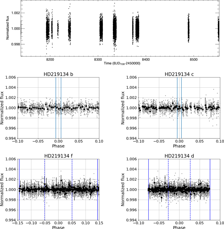
Figure 7. The ASTERIA detrended light curves for HD 219134. The top light curve shows all ASTERIA data used in the analysis presented here, plotted against BJD. The phase-folded data for HD 219134 b, c, f, and d, using planet periods from Gillon et al. (2017), are shown in the four smaller, lower panels. Gray points are 1-minute cadence data; black points are 20-minute binned data. The expected transit duration is shown as vertical blue bars for planets b and c; the 1σ (dashed blue) and 3σ (solid blue) transit windows are shown for planets f and d.
Download figure:
Standard image High-resolution image3.2. TESS Results and Discussion
The SPOC pipeline automatically detected the transits of HD 219134b and HD 219134c. The TESS Science Office designated the planets TOI 1469.01 and 1469.02 respectively. The known transits of HD 219134 b and c are clearly apparent in our detrended TESS two-minute cadence data (Figure 8).
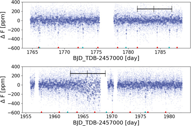
Figure 8. The TESS detrended HD 219134 light curve. Relative flux in ppm vs. time in days (units BJD). The light blue points are the detrended two-minute cadence data reduced from the SPOC target pixel stamps, and the dark blue points are data binned to 20 minutes. The transits are shown with triangles at the bottom of the plot, red for planet b and green for planet c. The 3σ transit window for planet f is shown as a black horizontal bar in the figures. Planet d is not expected to transit in the TESS observations within its 5σ transit window. Top: light curve from Sector 17. Bottom: light curve from Sector 24. Sector 24 has increased noise in its first orbit due to increased jitter from reduced frequency of momentum dumps.
Download figure:
Standard image High-resolution imageWe derived updated ephemerides for planets HD 219134 b and c using the MCMC method as implemented by the allesfitter code (Günther & Daylan 2020). In particular, we ran our MCMC routine with 100 walkers, 20000 steps, and a burn-in of 2000. For each free parameter, we ensured convergence by requiring that the chain lengths are at least 50 times the samplers autocorrelation time (Foreman-Mackey et al. 2013). The median and 1σ uncertainties of the posterior distributions, including the updated orbital periods and midtransit times are presented in detail in Table A3, with a summary of the midtransit times and periods in Table 3. We present the corresponding transit b and c fits in the Appendix.
Table 3. HD 219134 b and c Updated Midtransit Times (T0) and Planet Orbital Periods (P) from Our Detrended TESS SPOC Two-minute Cadence Data
| Planet Parameter | Planet b | Planet c |
|---|---|---|
| T0 (BJD) | 2458765.95501 ± 0.00047 |

|
| P (days) | 3.092920 ± 0.000011 |

|
Note. The values are median values with 1σ uncertainties.
Download table as: ASCIITypeset image
Beyond the known transits of HD 219134 b and c, no additional transits are detected in the SPOC light curves by the pipeline. We also find with our own detrended SPOC data that there are no obvious signs of any additional transit-like signals in the TESS Sectors 17 or 24 HD 219134 light curves.
Our TESS-data-derived radius lower limit for HD 219134 f is 1 R⊕, based on our injection and recovery tests (Section 2.4.2; Figure 9). This value is stringent enough to rule out transits.

Figure 9. Completeness in the TESS short-cadence light curves for HD 219134 planets f and d for different size planets. The y-axis represents the probability of detecting the planets of a given size if the transit occurred any time within the TESS observation data. The blue curve is for planet f and the orange curve is for planet d. The x-axis is planet radius in Earth radii. The error bars are estimated using the binomial distribution from 40 random draws of impact parameter and transit epochs. We can confidently rule out planet f transits as long as planet f is larger than 1 R⊕, which it is expected to be based on planet models for the maximum density of the minimum mass of planet f.
Download figure:
Standard image High-resolution imageOur derived lower limit of 1 R⊕ is smaller than the 1.3 R⊕ for a pure iron planet for HD 219134 f's radial-velocity minimum mass of  (e.g., Fortney et al. 2007; Seager et al. 2007; Zeng et al. 2016; Gillon et al. 2017). More specifically, we derive a lower limit of 0.925 R⊕ and 1.25 R⊕ for a 50% and 80% completeness in the recovery rate, respectively. With our derived lower radius limit smaller than any plausible planet, we thus rule out HD 219134 f as a transiting planet.
With a robust nondetection, we can state that, if real, that inclination of HD 219134 f is less than 886 (assuming we cannot detect a grazing transit).
TESS provides no constraint on HD 219134 d which did not pass through inferior conjunction during the TESS observations.
3.3. Transit-timing Variation Results and Discussion
From our TTV analysis (Section 2.5) we find no evidence that TTVs would have prevented either planet f or d from being detectable with the current recovery algorithms.
The TTV amplitude of HD 219134 f (Figure 6) could have been larger than the expected transit duration. However, since planet f should have transited once during the TESS data with a depth of about 238 ppm, it should have been detectable regardless of TTVs. Specifically we found that given the samples of orbital parameters, the distribution of TTVs ranges from 50 minutes to 350 minutes, larger than the expected transit duration of ≲230 minutes (Table 1).
The potential TTV amplitude of HD 219134 d (Figure 6) is smaller than the expected transit duration. More specifically we find that given the samples of orbital parameters, the distribution of TTVs ranges from 50 minutes to 250 minutes, less than the expected transit duration of ≲340 minutes (Table 1). Since the vast majority of TTV amplitudes are within the expected transit duration, TTVs most likely did not have an effect on the planet being observed.
A limitation to our TTV approach is that we used results from a Keplerian fit to infer TTV amplitudes that result from non-Keplerian dynamics. Another limitation is that both injection and recovery algorithms used linear ephemeris parameterization. One could push the TTV analysis to further accuracy by performing a full N-body photodynamical fit of the radial-velocity data and the photometry, including a non-Keplerian fit. Such an approach, however, is not warranted in the present paper because the expected transit depths of planets f and d are below the sensitivity threshold of ASTERIA.
4. Summary
We revisited the bright nearby star HD 219134 with TESS and ASTERIA. With the TESS data, we provided updated transit times and periods for the known transiting planets HD 219134 b and c. The planet f transit window fell within TESS Sector 17 and 24 data; we completely rule out transits for planet f based on the nondetection of planets smaller than a pure iron planet corresponding to the measured minimum mass of planet f.
We used the ASTERIA data to place upper limits on HD 219134 planet d transits (for which the transit window did not fall within the TESS data). ASTERIA was sensitive to planet d sizes down to a radius of 3.6 R⊕. There is still room for planet d to show transits, because planets within 10% of the mass of planet d's minimum mass have an empirical radius range from 1.7 to 7.0 R⊕.
ASTERIA was a technology demonstration mission that successfully achieved the pointing precision and thermal control necessary for precise photometry. Without design and calibration data for highly precise photometry, however, ASTERIA's residual uncorrelated noise ultimately limited the photometric precision and scientific capabilities. Nonetheless, ASTERIA technology demonstration success shows what is possible within a small satellite (specifically a CubeSat) platform.
ASTERIA data for HD 219134 is archived at https://exoplanetarchive.ipac.caltech.edu/docs/ASTERIAMission.html and TESS data for HD 219134 is archived at MAST (https://archive.stsci.edu/).
We acknowledge contributions from the extended team that supported ASTERIA development, integration and test, and operations, including Len Day, Maria de Soria Santacruz-Pich, Carl Felten, Janan Ferdosi, Kristine Fong, Harrison Herzog, Jim Hofman, David Kessler, Roger Klemm, Jules Lee, Jason Munger, Lori Moore, Esha Murty, Chris Shelton, David Sternberg, Rob Sweet, Kerry Wahl, Jacqueline Weiler, Thomas Werne, Shannon Zareh, and Ansel Rothstein-Dowden. We also recognize the JPL line organization and technical mentors for the expertise they provided throughout the project.
We thank the JPL program management, especially Sarah Gavit and Pat Beauchamp, who oversaw ASTERIA within the Engineering and Science Directorate at JPL. We also thank Daniel Coulter and Leslie Livesay for their support. The research was carried out in part at the Jet Propulsion Laboratory, California Institute of Technology, under a contract with the National Aeronautics and Space Administration. Government sponsorship acknowledged.
We would also like to thank the DSS-17 ground station team at Morehead State University (MSU) in Kentucky. We acknowledge the outstanding efforts of the student operators, technical staff, and program management at Morehead State University, including Chloe Hart, Sarah Wilczewski, Alex Roberts, Maria Lemaster, Lacy Wallace, Rebecca Mikula, Bob Kroll, Michael Combs, and Benjamin Malphrus.
Funding for the TESS mission is provided by NASA's Science Mission directorate. This paper includes data collected by the TESS mission, which are publicly available from the Mikulski Archive for Space Telescopes (MAST). Resources supporting this work were provided by the NASA High-End Computing (HEC) Program through the NASA Advanced Supercomputing (NAS) Division at Ames Research Center for the production of the SPOC data products. J.C.B. has been supported by the Heising-Simons 51 Pegasi b postdoctoral fellowship.
We acknowledge the Massachusett Tribe, the tribe of indigenous peoples from whom the Colony, Province, and Commonwealth of Massachusetts have taken their name. We would like to pay our respects to the ancestral bloodline of the Massachusett tribe and their descendants who still inhabit historical Massachusett tribe territories to this day.
Facilities: TESS - , ASTERIA - , MAST. -
Software: SPOC R4.0, QLP, Numpy (van der Walt et al. 2011), Scipy (Virtanen et al. 2020), Astropy (Astropy Collaboration et al. 2013, 2018), allesfitter (Günther & Daylan 2020), photutils (Bradley et al. 2019).
Appendix
The Appendix contains figures and tables to further describe HD 219134 properties (Table A1), ASTERIA data (Figure A1, Table A2), TESS data (Figure A2), and TESS data-derived HD 219134 planet and system parameters (Table A3).
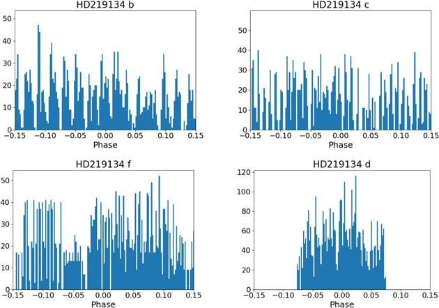
Figure A1. ASTERIA data density per planet phase (500 bins spaced uniformly in planet phase). The counts on the vertical axes are number of 1-minute cadence data points per bin.
Download figure:
Standard image High-resolution image
Figure A2. The TESS phase-folded light curves over the allesfitter best-fit orbital periods and midtransit times. (See Table A3). The gray points are the TESS unbinnned two-minute cadence data, the colored dots are the data binned over 15 minutes, and the red lines are 20 posterior models drawn randomly from the allesfitter posterior samples. The light-curve residuals are shown in the bottom panel.
Download figure:
Standard image High-resolution image
Table A1. Stellar Properties of HD 219134
| Property | Value | Source |
|---|---|---|
| R.A. (J2015.5; hh:mm:ss) | 23:13:16.780 | 1 |
| decl.. (J2015.5; dd:mm:ss) | +57:10:10.05 | 1 |
 (mas yr−1) (mas yr−1) |
2074.517 ± 0.137 | 1 |
 (mas yr−1) (mas yr−1) |
294.936 ± 0.123 | 1 |
| Parallax (mas) | 153.0808 ± 0.0895 | 1 |
| Distance (pc) | 6.5313 ± 0.0039 | 2 |
| Photometric Magnitudes | ||
| V (mag) | 5.570 ± 0.009 | 3 |
| B (mag) | 6.560 ± 0.007 | 3 |
| TESS (mag) | 4.628 ± 0.007 | 2 |
| Gaia (mag) | 5.2079 ± 0.0016 | 1 |
| J (mag) | 3.86 | 4 |
| H (mag) | 3.40 | 4 |
| Ks (mag) | 3.25 | 4 |
| Spectroscopic Properties | ||
 ( ( ) ) |
0.81 ± 0.03 | 5 |
 ( ( ) ) |
0.778 ± 0.005 | 7 |
| Teff (K) | 4700 ± 20 | 7 |
 (dex) (dex) |
4.567 ± 0.018 | 5 |
| [Fe/H] (dex) | 0.11 ± 0.04 | 6 |
 ( ( ) ) |
1.729 ± 0.073 | 5 |
 ( ( ) ) |
0.2646 ± 0.0050 | 5 |
| Age (Gyr) | 11.0 ± 2.2 | 5 |
Note. (1) Gaia DR2 (Gaia Collaboration et al. 2016 ). (2) TESS Input Catalog Version 8 (TICv8), Stassun et al. (2018). (3) Oja (1993). (4) Ducati (2002). (5) Gillon et al. (2017). (6) Motalebi et al. (2015). (7) Boyajian et al. (2012).
Download table as: ASCIITypeset image
Table A2. ASTERIA HD 219134 Observations Used in the Light Curve Shown in Figure 7
| Observation | First Frame | Last Frame | Number of | Number of 1-minute | Transit Window | rms |
|---|---|---|---|---|---|---|
| Name | [UTC] | [UTC] | Orbits | Integrations | [ppm/minute] | |
| Tech Demo 22 | 2018-01-20 06:26:38.6 | 2018-01-20 11:23:28.0 | 4 | 79 | None | 592 |
| (td22) | ||||||
| Science Observation 08 | 2018-03-14 10:18:11.4 | 2018-03-15 01:55:17.1 | 11 | 164 | f, d | 882 |
| (so08) | ||||||
| Science Observation 09 | 2018-03-15 09:22:26.2 | 2018-03-16 02:33:57.8 | 9 | 154 | f, d | 797 |
| (so09) | ||||||
| Science Observation 10 | 2018-03-16 14:53:01.3 | 2018-03-18 05:27:40.3 | 5 | 457 | f, d | 701 |
| (so10) | 2018-03-16 19:15:16.7 | 2018-03-18 05:25:40.3 | 19 | 747 | ||
| Science Observation 11 | 2018-03-19 07:17:15.5 | 2018-03-19 13:49:39.3 | 95 | b, d | 1023 | |
| (so11) | ||||||
| Science Observation 12 | 2018-03-20 07:54:53.9 | 2018-03-20 11:23:33.7 | 3 | 70 | c, d | 851 |
| (so12) | ||||||
| Science Observation 14 | 2018-03-25 09:49:25.5 | 2018-03-25 14:49:59.3 | 4 | 96 | b | 695 |
| (so14) | ||||||
| Science Observation 15 | 2018-03-26 21:11:51.1 | 2018-03-27 02:12:17.3 | 4 | 96 | c | 1038 |
| (so15) | ||||||
| Science Observation 18 | 2018-04-06 23:49:45.4 | 2018-04-08 15:57:33.8 | 21 | 101 | f | 601 |
| (so18) | ||||||
| Science Observation 21 | 2018-04-29 10:05:43.2 | 2018-04-29 14:48:51.3 | 3 | 177 | b, c, f, d | 624 |
| (so21) | 2018-04-29 20:52:26.2 | 2018-04-30 21:37:43.6 | 11 | 673 | ||
| 2018-05-01 03:40:17.5 | 2018-05-01 16:06:28.9 | 7 | 650 | |||
| Science Observation 22 | 2018-05-01 22:09:01.0 | 2018-05-02 04:25:39.3 | 3 | 264 | f, d | 585 |
| (so22) | 2018-05-02 10:28:05.4 | 2018-05-04 07:16:21.3 | 25 | 875 | ||
| Science Observation 37 | 2018-07-04 09:05:52.7 | 2018-07-05 16:07:55.4 | 18 | 534 | b, f | 695 |
| (so37) | 2018-07-05 20:28:50.8 | 2018-07-06 12:08:51.8 | 9 | 641 | ||
| Science Observation 38 | 2018-07-06 21:05:44.6 | 2018-07-07 06:35:35.0 | 6 | 732 | b, f | 617 |
| (so38) | 2018-07-07 12:28:46.6 | 2018-07-08 10:17:01.7 | 12 | 595 | ||
| 2018-07-08 14:37:54.9 | 2018-07-09 03:12:51.3 | 8 | 645 | |||
| Science Observation 39 | 2018-08-01 03:35:48.5 | 2018-08-02 18:23:49.6 | 19 | 309 | c, f, d | 720 |
| (so39) | ||||||
| Science Observation 40 | 2018-08-03 03:15:31.9 | 2018-08-03 14:20:30.9 | 7 | 1061 | b, d | 986 |
| (so40) | 2018-08-03 17:04:04.7 | 2018-08-04 05:43:21.2 | 9 | 682 | ||
| 2018-08-04 08:27:57.1 | 2018-08-05 04:45:39.2 | 12 | 710 | |||
| 2018-08-05 07:31:15.1 | 2018-08-06 13:03:45.5 | 19 | 715 | |||
| Science Observation 41 | 2018-08-07 01:03:01.7 | 2018-08-07 19:48:34.3 | 12 | 271 | d | 751 |
| (so41) | ||||||
| Science Observation 43 | 2018-09-10 14:10:58.7 | 2018-09-12 00:23:13.8 | 21 | 496 | b, f | 645 |
| (so43) | ||||||
| Science Observation 45 | 2018-09-17 07:43:57.2 | 2018-09-18 01:01:37.9 | 10 | 243 | b, d | 575 |
| (so45) | ||||||
| Science Observation 46 | 2018-09-18 09:51:37.5 | 2018-09-19 21:37:50.1 | 19 | 474 | d | 613 |
| (so46) | ||||||
| Science Observation 47 | 2018-09-20 08:00:54.7 | 2018-09-20 23:46:46.1 | 9 | 240 | b, d | 640 |
| (so47) | ||||||
| Science Observation 48 | 2018-09-21T05:32:52.0 | 2018-09-22 15:45:40.3 | 21 | 851 | b, d | 622 |
| (so48) | 2018-09-22T19:59:26.0 | 2018-09-24 00:02:48.8 | 15 | 589 | ||
| Science Observation 50 | 2019-01-04 15:45:39.4 | 2019-01-07 00:42:54.7 | 31 | 472 | c, f | 701 |
| (so50) | ||||||
| Science Observation 64 | 2019-03-08 13:04:22.6 | 2019-03-09 19:59:47.7 | 15 | 541 | None | 577 |
| (so64) | 2019-03-10 01:50:02.4 | 2019-03-11 02:36:50.7 | 10 | 502 | ||
Note. Observations designated "Tech Demo" or "td" took place during the initial phase of the mission when observations were focused on addressing ASTERIA's technology demonstration goals. After the technology demonstration objectives were completed, the naming scheme changed to "Science Observation" or "so" to indicate the change in focus from technology demonstration to collection of science data.
Table A3. Median Values and 1σ Uncertainties for the HD 219134b and HD 219134c Planets. The Planet Radii and Semimajor Axes Are Less Precise Than in Gillon et al. (2017)
| Parameter | HD 219134b | HD 219134c |
|---|---|---|
Midtransit Time,  (BJD days) (BJD days) |
2458765.95501 ± 0.00047 |
|
| Orbital Period, Pp (days) | 3.092920 ± 0.000011 |

|
Radius Ratio, 
|

|

|
Sum of Radii over Semimajor axis, 
|

|

|
Cosine of Orbital Inclination, 
|
0.0870 ± 0.0016 | 0.04703 ± 0.0010 |
Transit Depth,  (ppt) (ppt) |
|

|
Planet Radius, Rp ( ) ) |

|

|
| Semimajor Axis, ap (au) | 0.03863 ± 0.00062 | 0.0652 ± 0.0010 |
| Orbital Inclination, ip (deg) | 85.008 ± 0.091 | 87.304 ± 0.059 |
Impact Parameter, 
|

|

|
Total Transit Duration,  (h) (h) |

|

|
Full Transit Duration,  (h) (h) |

|

|
Equilibrium Temperature,  (K) (K) |
930.1 ± 7.6 | 715.9 ± 5.8 |
| System Parameters | ||
Limb-darkening Coefficient 1, 
|
0.66 ± 0.44 | |
Limb-darkening Coefficient 2, 
|

|
|
Flux Error,  ( ( ) ) |
−8.9024 ± 0.0040 | |
GP Characteristic Amplitude, 
|
−10.472 ± 0.056 | |
GP Timescale, 
|
−2.11 ± 0.21 | |
Download table as: ASCIITypeset image
Footnotes
- 18
The cotrending basis vectors can be downloaded from the MAST CBV bulk download page.
- 19