


Abstract
The growing field of large-scale time domain astronomy requires methods for probabilistic data analysis that are computationally tractable, even with large data sets. Gaussian processes (GPs) are a popular class of models used for this purpose, but since the computational cost scales, in general, as the cube of the number of data points, their application has been limited to small data sets. In this paper, we present a novel method for GPs modeling in one dimension where the computational requirements scale linearly with the size of the data set. We demonstrate the method by applying it to simulated and real astronomical time series data sets. These demonstrations are examples of probabilistic inference of stellar rotation periods, asteroseismic oscillation spectra, and transiting planet parameters. The method exploits structure in the problem when the covariance function is expressed as a mixture of complex exponentials, without requiring evenly spaced observations or uniform noise. This form of covariance arises naturally when the process is a mixture of stochastically driven damped harmonic oscillators—providing a physical motivation for and interpretation of this choice—but we also demonstrate that it can be a useful effective model in some other cases. We present a mathematical description of the method and compare it to existing scalable GP methods. The method is fast and interpretable, with a range of potential applications within astronomical data analysis and beyond. We provide well-tested and documented open-source implementations of this method in C++, Python, and Julia.
Export citation and abstract BibTeX RIS
1. Introduction
In the astrophysical literature, Gaussian processes (GPs; Rasmussen & Williams 2006) have been used to model stochastic variability in light curves of stars (Brewer & Stello 2009), active galactic nuclei (Kelly et al. 2014), and the logarithmic flux of X-ray binaries (Uttley et al. 2005). They have also been used as models for the cosmic microwave background (Bond & Efstathiou 1987; Bond et al. 1999; Wandelt & Hansen 2003), correlated instrumental noise (Gibson et al. 2012), and spectroscopic calibration (Evans et al. 2015; Czekala et al. 2017). While these models are widely applicable, their use has been limited, in practice, by the computational cost and scaling. The cost of computing a general GP likelihood scales as the cube of the number of data points  , and in the current era of large time domain surveys—with as many as ∼104–109 targets with ∼103–105 observations each—this scaling is prohibitive.
Existing astronomical time series data sets have already reached the limit where naïve application of GP models is no longer tractable. NASA's Kepler mission (Borucki et al. 2010), for example, measured light curves with more than 60,000 observations each for about 190,000 stars. Current and forthcoming surveys such as K2 (Howell et al. 2014), TESS(Ricker et al. 2014), LSST (Ivezić et al. 2008), WFIRST (Spergel et al. 2015), and PLATO (Rauer et al. 2014) will continue to produce similar or larger data volumes.
In this paper, we present a method for directly and exactly computing a class of GP models that scales linearly with the number of data points  for one-dimensional data sets. Unlike earlier linear methods using Kalman filters (e.g., Kelly et al. 2014), this novel algorithm exploits the semiseparable structure of a specific class of covariance matrices to directly factorize and solve the system. This method can only be used with one-dimensional data sets, and the covariance function must be represented by a mixture of exponentials; we will return to a discussion of what this means in detail in the following sections. However, the measurements do not need to be evenly spaced, and the uncertainties can be heteroscedastic.
This method achieves linear scaling by exploiting structure in the covariance matrix when it is generated by a mixture of exponentials. The semiseparable nature of these matrices was first recognized by Ambikasaran (2015), building on intuition from a 20 yr old paper (Rybicki & Press 1995). As we will discuss in the following pages, this choice of kernel function arises naturally in physical systems, and we demonstrate that it can be used as an effective model8 in other cases. This method is especially appealing compared to other similar methods—we discuss these comparisons in Section 7—because it is exact, simple, and fast.
Our main expertise lies in the field of exoplanet discovery and characterization where GPs have become a model of choice. We are confident that this method will benefit this field, but we also expect that there will be applications in other branches of astrophysics and beyond. In Section 6, we present applications of the method to research problems in stellar rotation (Section 6.3), asteroseismic analysis (Section 6.4), and exoplanet transit fitting (Section 6.5). Some readers might consider starting with this section for motivating examples before delving into the detailed derivations of the earlier sections.
In the following pages, we motivate the general problem of GP modeling, derive our novel direct solver, and demonstrate the model's application on real and simulated data sets. Alongside this paper, we have released well-tested and documented open-source implementations written in C++, Python, and Julia. These are available online at GitHub (https://github.com/dfm/celerite) and Zenodo.
2. Gaussian Processes
GPs are stochastic models consisting of a mean function  and a covariance, autocorrelation, or "kernel" function
  parameterized by
  and
and  , respectively. Under this model, the log-likelihood function
  with a data set

at coordinates

is

where

is the vector of residuals and the elements of the covariance matrix K are given by ![${[{K}_{{\boldsymbol{\alpha }}}]}_{{nm}}={k}_{{\boldsymbol{\alpha }}}({{\boldsymbol{x}}}_{n},{{\boldsymbol{x}}}_{m})$](https://content.cld.iop.org/journals/1538-3881/154/6/220/revision1/ajaa9332ieqn8.gif) . Equation (3) is the equation of an N-dimensional Gaussian, and it can be derived as the generalization of what we astronomers call "
. Equation (3) is the equation of an N-dimensional Gaussian, and it can be derived as the generalization of what we astronomers call " " to include the effects of correlated noise. A point estimate for the values of the parameters
  and
and  for a given data set
  can be found by maximizing Equation (3)—or the likelihood times a prior for a Bayesian estimate—with respect to
  and
and  using a nonlinear optimization routine (Nocedal & Wright 2006). Furthermore, the posterior probability density for
  and
and  can be quantified by multiplying the likelihood by a prior
  and using a Markov chain Monte Carlo (MCMC) algorithm to sample the joint posterior probability density.
GP models have been widely used across the physical sciences, but their application is generally limited to small data sets,  , because the cost of computing the inverse and determinant of a general matrix
  is
is  . In other words, this cost is proportional to the cube of the number of data points N. Furthermore, the storage requirements also scale as
  . This means that for large data sets every evaluation of the likelihood quickly becomes computationally intractable, and representing the matrix in memory can become expensive. In this case, the use of nonlinear optimization or MCMC is no longer practical.
This is not a purely academic concern. While the cost of directly evaluating the GP likelihood using a tuned linear algebra library9 with a data set of N = 1024 measurements is less than 1/10 of a second, the same calculation with N = 8192 takes over 8 s. Furthermore, most optimization and sampling routines are iterative, requiring many evaluations of this model to perform parameter estimation or inference. Existing data sets from astronomical surveys like Kepler and K2 include tens of thousands of observations for hundreds of thousands of targets, and upcoming surveys like LSST are expected to produce thousands or tens of thousands of measurements each for billions of astronomical sources (Ivezić et al. 2008). Scalable methods will be required if we ever hope to use GP models with these data sets.
In this paper, we present a method for improving the cubic scaling for some use cases. We call our method and its implementations celerite.10
The celerite method requires using a specific model for the covariance  , and although it has some limitations, we demonstrate in subsequent sections that it can increase the computational efficiency of many astronomical data analysis problems. The main limitation of this method is that it can only be applied to one-dimensional data sets, where by "one-dimensional" we mean that the input coordinates
  are scalar,
  . We use t as the input coordinate because one-dimensional GPs are often applied to time series data, but this is not a real restriction and the celerite method can be applied to any one-dimensional data set. Furthermore, the covariance function for the celerite method is "stationary." In other words,
  is only a function of
  .
.
3. The Celerite Model
To scale GP models to larger data sets, Rybicki & Press (1995) presented a method of computing the first term in Equation (3) in  operations when the covariance function is given by

where  are the measurement uncertainties,
  is the Kronecker delta, and
  . The intuition behind this method is that, for this choice of
  , the inverse of
  is tridiagonal and can be computed with a small number of operations for each data point. This model has been generalized to arbitrary mixtures of exponentials (e.g., Kelly et al. 2011)

In this case, the inverse is dense, but Equation (3) can still be evaluated with a scaling of  , where J is the number of components in the mixture (Kelly et al. 2014; Ambikasaran 2015). In Section 5, we build on previous work (Ambikasaran 2015) to derive a faster method with the same
  scaling that can be used when
  is positive definite.
This kernel function can be made even more general by introducing complex parameters  and
and  . In this case, the covariance function becomes

and, for this function, Equation (3) can still be evaluated with  operations. The details of this method and a few implementation considerations are outlined in Section 5, but we first discuss some properties of this covariance function.
By rewriting the exponentials in Equation (7) as sums of sine and cosine functions, we can see that the autocorrelation structure is defined by a mixture of quasi-periodic oscillators

For clarity, we refer to the argument within the sum as a "celerite term" for the remainder of this paper. The Fourier transform11 of this covariance function is the power spectral density (PSD) of the process, and it is given by

The physical interpretation of this model is not immediately obvious, and we return to a more general discussion shortly, but we start by considering some special cases.
If we set the imaginary amplitude bj for some component j to zero, that term of Equation (8) becomes

and the PSD for this component is

This is the sum of two Lorentzian or Cauchy distributions with width cj centered on  . This model can be interpreted intuitively as a quasi-periodic oscillator with amplitude Aj = aj, quality factor
  , and period
  .
.
Similarly, setting both bj and dj to zero, we get

with the PSD

This model is often called a "damped random walk" or Ornstein–Uhlenbeck process (in reference to the classic paper, Uhlenbeck & Ornstein 1930), and this is the kernel that was studied by Rybicki & Press (1992, 1995).
Finally, we note that the product of two terms of the form found inside the sum in Equation (8) can also be rewritten as a sum with updated parameters

where


Therefore, the method described in Section 5 can be used to perform scalable inference on large data sets for any model, where the kernel function is a sum or product of celerite terms.
4. Celerite as a Model of Stellar Variations
We now turn to a discussion of celerite as a model of astrophysical variability. A common concern in the context of GP modeling in astrophysics is the lack of physical motivation for the choice of kernel functions. Kernels are often chosen simply because they are popular, with little consideration of the impact of this decision. In this section, we discuss an exact physical interpretation of the celerite kernel that is applicable to many astrophysical systems, but especially the time variability of stars.
Many astronomical objects are variable on timescales determined by their physical structure. For phenomena such as stellar (asteroseismic) oscillations, variability is excited by noisy physical processes and grows most strongly at the characteristic timescale but is also damped owing to dissipation in the system. These oscillations are strong at resonant frequencies determined by the internal stellar structure, which are both excited and damped by convective turbulence.
To relate this physical picture to celerite, we consider the dynamics of a stochastically driven damped simple harmonic oscillator (SHO). The differential equation for this system is

where  is the frequency of the undamped oscillator, Q is the quality factor of the oscillator, and
  is a stochastic driving force. If
  is white noise, the PSD of this process is (Anderson et al. 1990)

where S0 is proportional to the power at  . The power spectrum in Equation (20) matches Equation (9) if

for  . For
. For  , Equation (20) can be captured by a pair of celerite terms with parameters

For these definitions, the kernel is

where  . Because of the damping, the characteristic oscillation frequency in this model, dj, for any finite quality factor
  , is not equal to the frequency of the undamped oscillator,
  .
.
The power spectrum in Equation (20) has several limits of physical interest:
- 1.
- 2.Substituting
 , Equation (20) becomeswith the corresponding covariance function (using Equations (8) and (22))or, equivalently (using Equations (8) and (21)),This covariance function is also known as the Matérn-3/2 function (Rasmussen & Williams 2006). This model cannot be directly evaluated using celerite because, as we can see from Equation (21), the parameter bj is infinite for. The limit in Equation (29), however, suggests that an approximate Matérn-3/2 covariance can be computed with celerite by using a small value of f in Equation (29). The required value of f will depend on the specific data set and the precision requirements for the inference, so we encourage users to test this approximation in the context of their research before using it.
 - 3.Finally, in the limit of large Q, the model approaches a high-quality oscillation with frequency and covariance function


Figure 1 shows a plot of the PSD for these limits and several other values of Q. From this figure, it is clear that for  the model has no oscillatory behavior and that for large Q the shape of the PSD near the peak frequency approaches a Lorentzian.

Figure 1. Left: power spectrum of a stochastically driven simple harmonic oscillator (Equation (20)) plotted for several values of the quality factor Q. For comparison, the dashed line shows the Lorentzian function from Equation (11) with  and normalized so that
  . Middle: corresponding autocorrelation functions with the same colors. Right: three realizations in arbitrary units from each model in the same colors.
Download figure:
Standard image High-resolution imageThese special cases demonstrate that the stochastically driven SHO provides a physically motivated model that is flexible enough to describe a wide range of stellar variations, and we give some specific examples in Section 6. Low  can capture granulation noise, and high
  is a good model for asteroseismic oscillations. In practice, we take a sum over oscillators with different values of Q, S0, and
  to give a sufficient accounting of the power spectrum of stellar time series. Since this kernel is exactly described by the exponential kernel, the likelihood (Equation (3)) can be evaluated for a time series with N measurements in
  operations using the celerite method described in the next section.
5. Semiseparable Matrices and Celerite
The previous two sections describe the celerite model and its physical interpretation. In this section, we derive a new scalable direct solver for covariance matrices generated by this model to compute the GP likelihood (Equation (3)) for large data sets. This method exploits the semiseparable structure of these matrices to compute their Cholesky factorization in  operations.
The relationship between the celerite model and semiseparable linear algebra was first recognized by Ambikasaran (2015) building on earlier work by Rybicki & Press (1995). Ambikasaran derived a scalable direct solver for any general semiseparable matrix and applied this method to celerite models with bj = 0 and dj = 0. The Ambikasaran (2015) method uses a factorization routine that can be applied to general semiseparable matrices. In other words, it can be applied to factorize matrices even if they are not positive definite. While preparing this paper, we generalized this method to include nonzero bj and dj, but all valid GP covariance matrices are symmetric and positive definite, so we can exploit this constraint to derive a Cholesky factorization algorithm. It turns out that this algorithm is more than an order of magnitude faster than the previously published method when applied to celerite models. In this and the following sections we derive this novel factorization algorithm, and in Appendix A we discuss methods for ensuring that the covariance matrix for a celerite model is positive definite.
To start, we define a rank-R semiseparable matrix as a matrix K where the elements can be written as

for some N × R-dimensional matrices U and V and an N × N-dimensional diagonal matrix A. This definition can be equivalently written as

where the  function extracts the strict lower triangular component of its argument and
  is the equivalent strict upper triangular operation. In this representation, rather than storing the full N × N matrix K, it is sufficient to only store the N × R matrices U and V and the N diagonal entries of A, for a total storage volume of
  floating point numbers. Given a semiseparable matrix of this form, the matrix–vector products and matrix–matrix products can be evaluated in
  operations. We include a summary of the key operations in Appendix B, but the interested reader is directed to Vandebril et al. (2007) for more details about semiseparable matrices in general.
5.1. Cholesky Factorization of Positive-definite Semiseparable Matrices
For our purposes, we want to compute the log-determinant of K and solve linear systems of the form  for
for  , where K is a rank-R semiseparable positive-definite matrix. These can both be computed using the Cholesky factorization of K:

where L is a lower triangular matrix with unit diagonal and D is a diagonal matrix. We use the Ansatz that L has the form

where I is the identity, U is the matrix from above, and W is an unknown N × R matrix. Combining this with Equation (33), we find the equation

which we can solve for W. Setting each element on the left-hand side of Equation (36) equal to the corresponding element on the right-hand side, we derive the following recursion relations:

where Sn is a symmetric R × R matrix and every element  . The computational cost of one iteration of the update in Equation (37) is
  , and this must be run N times—once for each row—so the total cost of this factorization scales as
  .
.
After computing the Cholesky factorization of this matrix K, we can also apply its inverse and compute its log-determinant in  and
and  operations, respectively. The log-determinant of K is given by

where, since K is positive definite,  for all n.
The inverse of K can be applied using the relationship

First, we solve for  using forward substitution

where  for all j. Then, using this result and backward substitution, we compute
  :
:

where  for all j. The total cost of the forward and backward substitution passes scales as
  .
.
The algorithm derived here is a general method for factorizing, solving, and computing the determinant of positive-definite rank-R semiseparable matrices. As we will show below, this method can be used to compute Equation (3) for celerite models. In practice, when K is positive definite and this method is applicable, we find that this method is about a factor of 20 faster than an optimized implementation of the earlier, more general method from Ambikasaran (2015).
5.2. Scalable Computation of Celerite Models
The celerite model described in Section 3 can be exactly represented as a rank  semiseparable matrix12
where the components of the relevant matrices are
semiseparable matrix12
where the components of the relevant matrices are

A naïve implementation of the algorithm in Equation (37) for this system will result in numerical overflow and underflow issues in many realistic cases because both U and V have factors of the form  , where t can be any arbitrarily large real number. This issue can be avoided by reparameterizing the semiseparable representation from Equation (42). We define the following preconditioned variables:

and the new set of variables

with the constraint

Using this parameterization, we find the following numerically stable algorithm to compute the Cholesky factorization of a celerite model:

As before, a single iteration of this algorithm requires  operations, and it is repeated N times for a total scaling of
  . Furthermore,
  and
and  can be updated in place and used to represent
  and
and  , giving a total memory footprint of
  floating point numbers.
The log-determinant of K can still be computed as in the previous section, but we must update the forward and backward substitution algorithms to account for the reparameterization in Equation (43). The forward substitution with the reparameterized variables is

where  for all j, and the backward substitution algorithm becomes

where  for all j. The only difference, when compared to Equations (40) and (41), is the multiplication by
  in the recursion relations for
  and
and  . As before, the computational cost of this solve scales as
  .
.
5.3. Performance
We have derived a novel and scalable method for computing the Cholesky factorization of the covariance matrices produced by celerite models. In this section, we demonstrate the numerical and computational performance of this algorithm.
First, we empirically confirm that the method solves systems of the form  to high numerical accuracy. The left panel of Figure 2 shows the L-infinity norm for the residual
  for a range of data set sizes N and numbers of terms J. For each pair of N and J we repeated the experiment 10 times with different randomly generated data sets and celerite parameters, and we averaged across experiments to remove some sampling noise from this figure. The numerical error introduced by our method increases weakly for larger data sets
  and roughly linearly with J.

Figure 2. Left: maximum numerical error introduced by the algorithm described in the text as a function of the number of celerite terms J and data points N. Each line corresponds to a different J, and the error increases with J as shown in the legend. Each point in this figure is the average result across 10 systems with randomly sampled parameters. Right: distribution of fractional error on the log-determinant of K computed using the algorithm described in the text compared to the algorithm implemented in NumPy (Van Der Walt et al. 2011) for the same systems shown in the left panel. This histogram only includes comparisons for  because standard methods become computationally expensive for larger systems.
Download figure:
Standard image High-resolution imageFor the experiments with small  , we also compared the log-determinant calculation to the result calculated using the general log-determinant function provided by the NumPy project (Van Der Walt et al. 2011), itself built on the LAPACK (Anderson et al. 1999) implementation in the Intel Math Kernel Library.13
The right panel of Figure 2 shows a histogram of the fractional error in the log-determinant calculation for each of the 480 experiments with
, we also compared the log-determinant calculation to the result calculated using the general log-determinant function provided by the NumPy project (Van Der Walt et al. 2011), itself built on the LAPACK (Anderson et al. 1999) implementation in the Intel Math Kernel Library.13
The right panel of Figure 2 shows a histogram of the fractional error in the log-determinant calculation for each of the 480 experiments with  . These results agree to about 10−15, and the error only weakly increases with N and J.
We continue by measuring the real-world computational efficiency of this method as a function of N and J. This experiment was run on a 2013 MacBook Pro with a dual 2.6 GHz Intel Core i5 processor, but we find similar performance on other platforms. The celerite implementation used for this test is the Python interface with a C++ back end, but there is little overhead introduced by Python, so we find similar performance using the implementation in C++ and an independent implementation in Julia (Bezanzon et al. 2017). Figure 3 shows the computational cost of evaluating Equation (3) using celerite as a function of N and J. The empirical scaling as a function of data size matches the theoretical scaling of  for all values of N, and the scaling with the number of terms is the theoretical
  for
for  , with some overhead for smaller models. For comparison, the computational cost of the same computation using the Intel Math Kernel Library, a highly optimized general dense linear algebra package, is shown as a dashed line, which is independent of J. Celerite is faster than the reference implementation for all but the smallest data sets with many terms,
  for
for  , and J increasing with larger N.

Figure 3. Benchmark showing the computational scaling of celerite using the Cholesky factorization routine for rank- semiseparable matrices as described in the text. Left: cost of computing Equation (3) with a covariance matrix given by Equation (8) as a function of the number of data points N. The different lines show the cost for different numbers of terms J increasing from bottom to top. To guide the eye, the straight black line without points shows linear scaling in N. For comparison, the computational cost for the same model using a general Cholesky factorization routine implemented in the Intel MKL linear algebra package is shown as the dashed black line. Right: same information as in the left panel, plotted as a function of J for different values of N. Each line shows the scaling for a specific value of N increasing from bottom to top. The black line shows quadratic scaling in J.
Download figure:
Standard image High-resolution image5.4. How to Choose a Celerite Model
In any application of celerite—or any other GP model, for that matter—we must choose a kernel. A detailed discussion of model selection is beyond the scope of this paper, and the interested reader is directed to chapter 5 of Rasmussen & Williams (2006) for an introduction in the context of GPs, but we include a summary and some suggestions specific to celerite here.
For many of the astrophysics problems that we will tackle using celerite, it is possible to motivate the kernel choice physically. We give three examples of this in the next section, and in these cases we have a physical description of the system that generated our data, we represent that system as a celerite model, and we use celerite for parameter estimation. For other projects, we might be interested in comparing different theories, and in those cases we would need to perform formal model selection.
Sometimes, it is not possible to choose a physically motivated kernel when we use a GP as an effective model. In these cases, we recommend starting with a mixture of stochastically driven damped SHOs (as discussed in Section 4) and selecting the number of oscillators using Bayesian model comparison, cross-validation, or another model selection technique. Despite the fact that it is less flexible than a general celerite kernel, we recommend the SHO model in most cases because it is once mean square differentiable

giving smoother functions than the general celerite model, which is only mean square continuous.
For a similar class of models (we return to these below in Section 7) Kelly et al. (2014) recommend using an "information criterion," such as the Akaike information criterion (AIC) or the Bayesian information criterion (BIC), as a model selection metric. These criteria are easy to implement, and we use the BIC in Section 6.2, but each information criterion comes with caveats that should be considered in any application (see, e.g., Ivezić et al. 2014).
6. Examples
To demonstrate the application of celerite, we use it to perform posterior inference in two examples with realistic simulated data and three examples of real-world research problems. These examples have been chosen to justify the use of celerite for a range of research problems, but they are by no means exhaustive. These examples are framed in the time domain with a clear bias in favor of large homogeneous photometric surveys, but celerite can also be used for other one-dimensional problems such as spectroscopy, where wavelength—instead of time—is the independent coordinate (see Czekala et al. 2017, for a potential application).
In the first example, we demonstrate that celerite can be used to infer the power spectrum of a process when the data are generated from a celerite model. In the second example, we demonstrate that celerite can be used as an effective model even if the true process cannot be represented in the space of allowed models. This is an interesting example because, when analyzing real data, we rarely have any fundamental reason to believe that the data were generated by a GP model with a specific kernel. Even in these cases, GPs can be useful effective models, and celerite provides computational advantages over other GP methods.
The next three examples show celerite used to infer the properties of stars and exoplanets observed by NASA's Kepler mission. Each of these examples touches on an active area of research, so we limit our examples to be qualitative in nature and do not claim that celerite is the optimal method, but we hope that these examples encourage interested readers to investigate the applicability of celerite to their research.
In each example, the joint posterior probability density is given by

where  is the GP likelihood defined in Equation (3) and
  is the joint prior probability density for the parameters. We sample each posterior density using MCMC and investigate the performance of the model when used to interpret the physical processes that generated the data. The specific parameters and priors are discussed in detail in each section, but we generally assume independent uniform priors with plausibly broad support.
While we do perform a convergence analysis in each case by computing the autocorrelation function and integrated autocorrelation time for the target chain (Sokal 1989; Goodman & Weare 2010), the usual caveats associated with MCMC analysis apply when interpreting these results. For example, if there are multiple posterior modes that are not sampled by any chain, the autocorrelation analysis will not identify that the sampler has not converged. There are published sampling algorithms (Gregory 2005; Liu 2008; Feroz et al. 2009; Brewer et al. 2011; Kelly et al. 2014) that can, in some cases, be less sensitive to multimodality than the sampler that we use (Goodman & Weare 2010; Foreman-Mackey et al. 2013), but a comparison of sampling algorithms is beyond the scope of this paper, and celerite will also improve the computational efficiency of GP models when using the other inference algorithms.
6.1. Example 1: Recovery of a Celerite Process
In this first example, we simulate a data set using a known celerite process and fit it with celerite to show that valid inferences can be made in this idealized case. We simulate a small ( ) data set using a GP model with an SHO kernel (Equation (23)) with parameters
  , and
, and  , where the units are arbitrarily chosen to simplify the discussion. We add further white noise with the amplitude
  to each data point. The simulated data are plotted in the top left panel of Figure 4.

Figure 4. Top left: simulated data set (black error bars) and MAP model (blue contours). Bottom left: residuals between the mean predictive model and the data shown in the top left panel. Right: inferred PSD (the blue contours encompass 68% of the posterior mass) compared to the true PSD (dashed black line).
Download figure:
Standard image High-resolution imageIn this case, when simulating and fitting, we set the mean function  to zero—this means that the parameter vector
  is empty—and the elements of the covariance matrix are given by Equation (23) with three parameters
  . We choose a proper separable prior for
  with log-uniform densities for each parameter as listed in Table 1.


To start, we estimate the maximum a posteriori (MAP) parameters using the L-BFGS-B nonlinear optimization routine (Byrd et al. 1995; Zhu et al. 1997) implemented by the SciPy project (Jones et al. 2001). The top left panel of Figure 4 shows the mean and standard deviation of the predicted noise-free data distribution from the MAP model overplotted as a blue contour on the simulated data, and the bottom panel shows the residuals away from this model. Since we are using the correct model to fit the data, it is reassuring that the residuals appear qualitatively uncorrelated in this figure.
We then sample the joint posterior probability (Equation (50)) using emcee (Goodman & Weare 2010; Foreman-Mackey et al. 2013). We initialize 32 walkers14 by sampling from a three-dimensional isotropic Gaussian centered on the MAP parameter vector and with a standard deviation of 10−4 in each dimension. We then run 500 steps of burn-in and 2000 steps of MCMC. To assess convergence, we estimate the integrated autocorrelation time of the chain averaged across parameters (Sokal 1989; Goodman & Weare 2010) and find that the chain results in 1737 effective samples.
Each sample in the chain corresponds to a model PSD, and we compare this posterior constraint on the PSD to the true spectral density in the right panel of Figure 4. In this figure, the true PSD is plotted as a dashed black line, and the numerical estimate of the posterior constraint on the PSD is shown as a blue contour indicating 68% of the MCMC samples. It is clear from this figure that, as expected, the inference correctly reproduces the true PSD.
6.2. Example 2: Inferences with the "Wrong" Model
In this example, we simulate a data set using a known GP model with a kernel outside of the support of a celerite process. This means that the true autocorrelation of the process can never be correctly represented by the model that we are using to fit, but we use this example to demonstrate that, at least in this case, valid inferences can still be made about the physical parameters of the model.
The data are simulated from a quasi-periodic GP with the kernel

where Ptrue is the fundamental period of the process. This autocorrelation structure corresponds to the power spectrum (Wilson & Adams 2013)

which, for large values of ω, falls off exponentially. When compared to Equation (9)—which, for large ω, goes as  at most—it is clear that a celerite model can never exactly reproduce the structure of this process. That being said, we demonstrate that robust inferences can be made about Ptrue even with this effective model.
We generate a realization of a GP model with the kernel given in Equation (51) with  ,
,  s, and
  . We also add white noise with amplitude
  to each data point. The top left panel of Figure 5 shows this simulated data set.

Figure 5. Top left: simulated data set (black error bars) and MAP model (blue contours). Bottom left: residuals between the mean predictive model and the data shown in the top left panel. Right: inferred period of the process. The true period is indicated by the vertical gray line, the posterior inference using the correct model is shown as the blue dashed histogram, and the inference made using the "wrong" effective model is shown as the black histogram.
Download figure:
Standard image High-resolution imageWe then fit these simulated data using the product of two SHO terms (Equation (23)) where one of the terms has  and
and  fixed. The kernel for this model is

where kSHO is defined in Equation (23) and the period of the process is  . We note that, using Equation (14), the product of two celerite terms can also be expressed using celerite.
We choose this functional form by comparing the BIC for a set of different models. In each model, we take the sum or product of J SHO terms, find the maximum likelihood model using L-BFGS-B, and compute the BIC (Schwarz et al. 1978),

where  is the value of the likelihood at maximum, K is the number of parameters, and N is the number of data points. Figure 6 shows the value of the BIC for a set of products and sums of SHO terms, and the model that we choose has the lowest BIC.
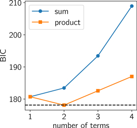
Figure 6. Bayesian information criterion (BIC) evaluated for the data from Figure 5 and different kernel choices. The x-axis shows the number of terms included in each model. The blue circles show models where the terms have been summed, and the orange squares indicate that the model is a product of terms. In the product models, the parameters S0 and Q are held fixed at 1 and  , respectively, for all but the first term. The dashed black line shows the minimum value of the BIC, and this corresponds to the model chosen in the text.
Download figure:
Standard image High-resolution imageAs in the previous example, we set the mean function to zero and can, therefore, omit the parameters  . Table 2 lists the proper log-uniform priors that we choose for each parameter in
  . These priors, together with the GP likelihood (Equation (3)), fully specify the posterior probability density.


As above, we estimate the MAP parameters using L-BFGS-B and sample the posterior probability density using emcee. The top left panel of Figure 5 shows the conditional mean and standard deviation of the MAP model. The bottom left panel shows the residuals between the data and this MAP model, and even though this GP model is formally "wrong," there are no obvious correlations in these residuals.
To perform posterior inference, we initialize 32 walkers by sampling from the four-dimensional Gaussian centered on the MAP parameters with an isotropic standard deviation of 10−4. We then run 500 steps of burn-in and 2000 steps of MCMC. To estimate the number of independent samples, we estimate the integrated autocorrelation time of the chain for the parameter  —the parameter of primary interest—and find 1134 effective samples.
For comparison, we run the same number of steps of MCMC to sample the "correct" joint posterior density. For this reference inference, we use a GP likelihood with the kernel given by Equation (51) and choose log-uniform priors on each of the three parameters  ,
,  , and
, and  .
.
The marginalized posterior inferences of the characteristic period of the process are shown in the right panel of Figure 5. The inference using the correct model is shown as a dashed blue histogram, and the inference made using the effective model is shown as a solid black histogram. These inferences are consistent with each other and with the true period used for the simulation (shown as a vertical gray line). This demonstrates that, in this case, celerite can be used as a computationally efficient effective model, and hints that this may be true in other problems as well.
6.3. Example 3: Stellar Rotation
A source of variability that can be measured from time series measurements of stars is rotation. The inhomogeneous surface of the star (spots, plage, etc.) imprints itself as quasi-periodic variations in photometric or spectroscopic observations (Dumusque et al. 2014). It has been demonstrated that for light curves with nearly uniform sampling the empirical autocorrelation function provides a reliable estimate of the rotation period of a star (McQuillan et al. 2013, 2014; Aigrain et al. 2015) and that a GP model with a quasi-periodic covariance function can be used to make probabilistic measurements even with sparsely sampled data (Angus et al. 2017). The covariance function used for this type of analysis has the form

where Prot is the rotation period of the star. GP modeling with the same kernel function has been proposed as a method of measuring the mean periodicity in quasi-periodic photometric time series in general (Wang et al. 2012). The key difference between Equation (55) and other quasi-periodic kernels is that it is positive for all values of τ. We construct a simple celerite covariance function with similar properties as follows:

for  , and
, and  . The covariance function in Equation (56) cannot exactly reproduce Equation (55), but since Equation (55) is only an effective model, Equation (56) can be used as a drop-in replacement for a significant gain in computational efficiency.
GPs have been used to measure stellar rotation periods for individual data sets (e.g., Littlefair et al. 2017), but the computational cost of traditional GP methods has hindered the industrial application to existing surveys like Kepler with hundreds of thousands of targets. The increase in computational efficiency and scalability provided by celerite opens the possibility of inferring rotation periods using GPs at the scale of existing and forthcoming surveys like Kepler, TESS, and LSST.
As a demonstration, we fit a celerite model with a kernel given by Equation (56) to a Kepler light curve for the star KIC 1430163. This star has a published rotation period of  , measured using traditional periodogram and autocorrelation function approaches applied to Kepler data from Quarters 0–16 (Mathur et al. 2014), covering about 4 yr.
We select about 180 days of contiguous observations of KIC 1430163 from Kepler. This data set has 6950 measurements, and, using a tuned linear algebra implementation,15
a single evaluation of the likelihood requires over 8 s on a modern Intel CPU. This calculation, using celerite with the model in Equation (56), only takes  —a speed-up of more than three orders of magnitude per model evaluation.
We set the mean function  to zero, and the remaining parameters
  and their priors are listed in Table 3. As with the earlier examples, we start by estimating the MAP parameters using L-BFGS-B and initialize 32 walkers by sampling from an isotropic Gaussian with a standard deviation of 10−5 centered on the MAP parameters. The left panels of Figure 7 show a subset of the data used in this example and the residuals away from the MAP predictive mean.

Figure 7. Inferred constraints on a quasi-periodic GP model using the covariance function in Equation (56) and two quarters of Kepler data. Top left: Kepler data (black points) and the MAP model prediction (blue curve) for a 60-day subset of the data used. The solid blue line shows the predictive mean, and the blue contours show the predictive standard deviation. Bottom left: residuals between the mean predictive model and the data shown in the top left figure. Right: posterior constraint on the rotation period of KIC 1430163 using the data set and model from Figure 7. The period is the parameter Prot in Equation (56), and this figure shows the posterior distribution marginalized over all other nuisance parameters in Equation (56). The 1σ error bar on this measurement is indicated with vertical dashed lines. This result is consistent with the published rotation period made using the full Kepler baseline, shown as a vertical gray line (Mathur et al. 2014).
Download figure:
Standard image High-resolution image


We run 500 steps of burn-in, followed by 5000 steps of MCMC using emcee. We estimate the integrated autocorrelation time of the chain for  and estimate that we have 2900 independent samples. These samples give a posterior constraint on the period of
  days, and the marginalized posterior distribution for P is shown in the right panel of Figure 7. This result is in good agreement with the literature value with smaller uncertainties. A detailed comparison of GP rotation period measurements and the traditional methods is beyond the scope of this paper, but Angus et al. (2017) demonstrate that GP inferences are, at a population level, more reliable than other methods.
The total computational cost for this inference using celerite is about 4 CPU minutes. By contrast, the same inference using a general but optimized Cholesky factorization routine would require nearly 400 CPU hours. This speed-up enables probabilistic measurement of rotation periods using existing data from K2 and forthcoming surveys like TESS and LSST, where this inference will need to be run for at least hundreds of thousands of stars.
6.4. Example 4: Asteroseismic Oscillations
The asteroseismic oscillations of thousands of stars were measured using light curves from the Kepler mission (Gilliland et al. 2010; Chaplin et al. 2011, 2013; Huber et al. 2011; Stello et al. 2013), and asteroseismology is a key science driver for many of the upcoming large-scale photometric surveys (Rauer et al. 2014; Gould et al. 2015; Campante et al. 2016). Most asteroseismic analyses have been limited to high signal-to-noise oscillations because the standard methods use statistics of the empirical periodogram. These methods cannot formally propagate the measurement uncertainties to the constraints on physical parameters, and they instead rely on population-level bootstrap uncertainty estimates (Huber et al. 2009). More sophisticated methods that compute the likelihood function in the time domain scale poorly to large survey data sets (Brewer & Stello 2009; Corsaro & Ridder 2014).
Celerite alleviates these problems by providing a physically motivated probabilistic model that can be evaluated efficiently even for large data sets. In practice, we model the star as a mixture of stochastically driven SHOs where the amplitudes and frequencies of the oscillations are computed using a physical model, and we evaluate the probability of the observed time series using a GP where the PSD is a sum of terms given by Equation (20). This gives us a method for computing the likelihood function for the parameters of the physical model (e.g.,  and
and  , or other more fundamental parameters) conditioned on the observed time series in
  operations. In other words, celerite provides a computationally efficient framework that can be combined with physically motivated models of stars and numerical inference methods to make rigorous probabilistic measurements of asteroseismic parameters in the time domain. This has the potential to push asteroseismic analysis to lower signal-to-noise data sets, and we hope to revisit this idea in a future paper.
To demonstrate the method, we use a simple heuristic model where the PSD is given by a mixture of eight components with amplitudes and frequencies specified by  , and some nuisance parameters. The first term is used to capture the granulation "background" (Kallinger et al. 2014) using Equation (24) with two free parameters Sg and
  . The remaining seven terms are given by Equation (20), where Q is a nuisance parameter shared between terms, the frequencies are given by

and the amplitudes are given by

where j is an integer running from −3 to 3 and  , and W are shared nuisance parameters. Finally, we also fit for the amplitude of the white noise by adding a parameter σ in quadrature with the uncertainties given for the Kepler observations. All of these parameters and their chosen priors are listed in Table 4. As before, these priors are all log-uniform except for
  , where we use a zero-mean normal prior with a broad variance of
  to break the degeneracy between
  and . To build a more realistic model, this prescription could be extended to include more angular modes, or
  and
and  could be replaced by the fundamental physical parameters of the star.


To demonstrate the applicability of this model, we apply it to infer the asteroseismic parameters of the giant star KIC 11615890, observed by the Kepler mission. The goal of this example is to show that, even for a low signal-to-noise data set with a short baseline, it is possible to infer asteroseismic parameters with formal uncertainties that are consistent with the parameters inferred with a much larger data set. Looking forward to TESS(Ricker et al. 2014; Campante et al. 2016), we measure  and
and  using only 1 month of Kepler data and compare our results to the results inferred from the full 4 yr baseline of the Kepler mission. For KIC 11615890, the published asteroseismic parameters measured using several years of Kepler observations are (Pinsonneault et al. 2014)

Unlike typical giants, KIC 11615890 is a member of a class of stars where the dipole ( ) oscillation modes are suppressed by strong magnetic fields in the core (Stello et al. 2016). This makes this target simpler for the purposes of this demonstration because we can neglect the
  modes and the model proposed above will be an effective model for the combined signal from the
  and 2 modes.
For this demonstration, we randomly select a month-long segment of PDC Kepler data (Smith et al. 2012; Stumpe et al. 2012). Unlike the previous examples, the posterior distribution is sharply multimodal, and naïvely maximizing the posterior using L-BFGS-B is not practical. Instead, we start by estimating the initial values for  and
and  using only the month-long subset of data and following the standard procedure described by Huber et al. (2009). We then run a set of L-BFGS-B optimizations with values of
  selected in a logarithmic grid centered on our initial estimate of
  and initial values of
  computed using the empirical relationship between these two quantities (Stello et al. 2009). This initialization procedure is sufficient for this example, but the general application of this method will require a more sophisticated prescription.
Figure 8 shows a 10-day subset of the data set used for this example. The MAP model is overplotted on these data, and the residuals away from the mean prediction of this model are shown in the bottom panel of Figure 8. There is no obvious structure in these residuals, lending some credibility to the model specification.

Figure 8. Top: Kepler data (black points) and the MAP model prediction (blue curve) for a 10-day subset of the month-long data set that was used for the fit. The solid blue line shows the predictive mean, and the blue contours show the predictive standard deviation. Bottom: residuals between the mean predictive model and the data shown in the top figure.
Download figure:
Standard image High-resolution imageWe initialize 32 walkers by sampling from an isotropic Gaussian centered on the MAP parameters (the full set of parameters and their priors are listed in Table 4), run 5000 steps of burn-in, and run 15,000 steps of MCMC using emcee. We estimate the mean autocorrelation time for the chains of  and
and  and find 1443 effective samples from the marginalized posterior density. Figure 9 shows the marginalized density for
  and
and  compared to the results from the literature. This result is consistent within the published error bars, and the posterior constraints are tighter than the published results. The top two panels of Figure 10 show the Lomb–Scargle periodogram (VanderPlas 2017) estimator for the power spectrum based on the full 4 yr of Kepler data and the month-long subset used in our analysis. The bottom panel of Figure 10 shows the posterior inference of the PSD using the celerite and the model described here. Despite only using 1 month of data, the celerite inference captures the salient features of the power spectrum, and it is qualitatively consistent with the standard estimator applied to the full baseline. All asteroseismic analyses are known to have substantial systematic and method-dependent uncertainties (Verner et al. 2011), so further experiments would be needed to fully assess the reliability of this specific model.

Figure 9. Probabilistic constraints on  and
and  from the inference shown in Figure 8 compared to the published value (blue error bars) based on several years of Kepler observations (Pinsonneault et al. 2014). The two-dimensional contours show the 0.5σ, 1σ, 1.5σ, and 2σ credible regions in the marginalized planes, and the histograms along the diagonal show the marginalized posterior for each parameter.
Download figure:
Standard image High-resolution image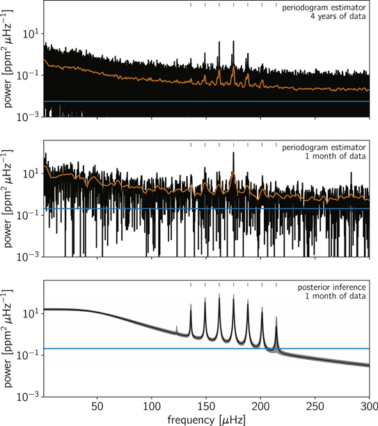
Figure 10. Comparison between the Lomb–Scargle estimator of the PSD and the posterior inference of the PSD as a mixture of stochastically driven simple harmonic oscillators. Top: periodogram of the Kepler light curve for KIC 11615890 computed on the full 4 yr baseline of the mission. The orange line shows a smoothed periodogram, and the blue line indicates the level of the measurement uncertainties. Middle: same periodogram computed using about a month of data. Bottom: power spectrum inferred using the mixture of SHOs model described in the text and only 1 month of Kepler data. The black line shows the median of posterior PSD, and the gray contours show the 68% credible region.
Download figure:
Standard image High-resolution imageFor this example, about 10 CPU minutes were required to run the MCMC. This is more computationally intensive than traditional methods of measuring asteroseismic oscillations, but it is much cheaper than the same analysis using a general direct GP solver. For comparison, we estimate that repeating this analysis using a general Cholesky factorization implemented as part of a tuned linear algebra library16 would require about 15 CPU hours. An in-depth discussion of the benefits of rigorous probabilistic inference of asteroseismic parameters in the time domain is beyond the scope of this paper, but we hope to revisit this opportunity in the future.
6.5. Example 5: Exoplanet Transit Fitting
This example is different from all the previous examples—both simulated and real—because, in this case, we do not set the mean function  to zero. Instead, we make inferences about
  because it is a physically significant function and the parameters are fundamental properties of the system. This is an example using real data—because we use the light curve from Section 6.3—but we multiply these data by a simulated transiting exoplanet model with known parameters. This allows us to show that we can recover the true parameters of the planet even when the transit signal is superimposed on the real variability of a star. GP modeling has been used extensively for this purpose throughout the exoplanet literature (e.g., Dawson et al. 2014; Barclay et al. 2015; Evans et al. 2015; Foreman-Mackey et al. 2016; Grunblatt et al. 2016).
In Equation (3) the physical parameters of the exoplanet are called  , and in this example the mean function
  is a limb-darkened transit light curve (Mandel & Agol 2002; Foreman-Mackey & Morton 2016) and the parameters
  are the orbital period Porb, the transit duration T, the phase or epoch t0, the impact parameter b, the radius of the planet in units of the stellar radius
  , the baseline relative flux of the light curve f0, and two parameters describing the limb-darkening profile of the star (Claret & Bloemen 2011; Kipping 2013). As in Section 6.3, we model the stellar variability using a GP model with a kernel given by Equation (56) and fit for the parameters of the exoplanet
  and the stellar variability
  simultaneously. The full set of parameters
  and
and  is listed in Table 5, along with their priors and the true values for
  .
.
Table 5. Parameters, Priors, and (if Known) the True Values Used for the Simulation in Example 5
| Parameter | Prior | True Value |
|---|---|---|
Kernel: 
|
||

|

|
⋯ |

|

|
⋯ |

|

|
⋯ |

|

|
⋯ |

|

|
⋯ |
Mean: 
|
||

|

|
0 |

|

|

|

|

|

|

|

|

|

|

|
0 |
| b |

|
0.5 |
| q1 |

|
0.5 |
| q2 |

|
0.5 |
Download table as: ASCIITypeset image
We take a 20-day segment of the Kepler light curve for KIC 1430163 ( ) and multiply it by a simulated transit model with the parameters listed in Table 5. Using these data, we maximize the joint posterior defined by the likelihood in Equation (3) and the priors in Table 5 using L-BFGS-B for all the parameters
  and
and  simultaneously. The top panel of Figure 11 shows the data including the simulated transit as black points, with the MAP model prediction overplotted in blue. The bottom panel of Figure 11 shows the "detrended" light curve, where the MAP model has been subtracted and the MAP mean model
  has been added back in. For comparison, the transit model is overplotted in the bottom panel of Figure 11, and we see no obvious correlations in the residuals.

Figure 11. Top: month-long segment of the Kepler light curve for KIC 1430163 with a synthetic transit model injected (black points) and the MAP model for the stellar variability (blue line). Bottom: MAP "detrending" of the data in the top panel. In this panel, the MAP model for the stellar variability has been subtracted to leave only the transits. The detrended light curve is shown by black error bars, and the MAP transit model is shown as a blue line.
Download figure:
Standard image High-resolution imageSampling 32 walkers from an isotropic Gaussian centered on the MAP parameters, we run 10,000 steps of burn-in and 30,000 steps of production MCMC using emcee. We estimate the integrated autocorrelation time for the  chain and find 1490 effective samples across the full chain. Figure 12 shows the marginalized posterior constraints on the physical properties of the planet compared to the true values. Even though the celerite representation of the stellar variability is only an effective model, the inferred distributions for the physical properties of the planet
  are consistent with the true values. This promising result suggests that celerite can be used as an effective model for transit inference for a significant gain in computational tractability. Even for this example with small N, the cost of computing the likelihood using celerite is nearly two orders of magnitude faster than the same computation using a general direct solver.

Figure 12. Marginalized posterior constraints on the physical parameters of the planet transit in the light curve shown in the top panel of Figure 11. The two-dimensional contours show the 0.5σ, 1σ, 1.5σ, and 2σ credible regions in the marginalized planes, and the histograms along the diagonal show the marginalized posterior for each parameter. The true values used in the simulation are indicated by blue lines. For each parameter, the inference is consistent with the true value.
Download figure:
Standard image High-resolution image6.6. Summary
In the previous subsections, we demonstrate five potential use cases for celerite. These examples span a range of data sizes and model complexities, and the last three are based on active areas of research with immediate real-world applicability. The sizes of these data sets are modest on the scale of some existing and forthcoming survey data sets because we designed the experiments to be easily reproducible, but, even in these cases, the inferences made here would be intractable without substantial computational investment.
Table 6 lists the specifications of each example. In this table, we list the computational cost required for a single likelihood evaluation using a general Cholesky factorization and the cost of computing the same likelihood using celerite. Combining this with the total number of model evaluations required to run the MCMC algorithm to convergence (this number is also listed in Table 6), we can estimate the total CPU time required in each case. While the exact computational requirements for any problem also depend on the choice of inference algorithm and the specific precision requirements, this table provides a rough estimate of what to expect for projects at these scales.
Table 6. Computational Cost and Convergence Stats for Each Example
| N | J | Directa | Celeriteb | Dimensionc | Evaluationsd | Neffe | |
|---|---|---|---|---|---|---|---|
| (ms) | (ms) | ||||||
| 1 | 200 | 1 | 2.85 | 0.26 | 3 | 80,000 | 1737 |
| 2 | 100 | 2 | 0.67 | 0.36 | 4 | 80,000 | 1134 |
| 3 | 6950 | 2 | 8119.11 | 1.47 | 4 | 176,000 | 2900 |
| 4 | 1440 | 8 | 828.93 | 2.74 | 9 | 640,000 | 1443 |
| 5 | 1000 | 2 | 88.30 | 0.96 | 13 | 1,280,000 | 1490 |
Notes.
aThe computational cost of computing the GP model using the general Cholesky factorization routine implemented in the Intel MKL. bThe computational cost of computing the GP model using celerite. cThe total number of parameters in the model. dThe total number of evaluations of the model to run MCMC to convergence. eThe effective number of independent samples estimated by computing the integrated autocorrelation time of the chain.Download table as: ASCIITypeset image
7. Comparisons to Other Methods
There are other methods of scaling GP models to large data sets, and in this section we draw comparisons between celerite and other popular methods. Scalable GP methods tend to fall into two categories: approximate and restrictive. Celerite falls into the latter category because, while the method is exact, it requires a specific choice of stationary kernel function and can only be used in one dimension.
The continuous autoregressive moving average (CARMA) models introduced to the astrophysics literature by Kelly et al. (2014) share many features with celerite. CARMA models are restricted to one-dimensional problems, and the likelihood function for a CARMA model can be solved in  using a Kalman filter (Kelly et al. 2014). The kernel function for a CARMA
  model is

where

and  and
and  are parameters of the model; σ is real, while the others are complex. Comparing Equation (60) to Equation (7), we can see that every CARMA model corresponds to an equivalent celerite model and the parameters
  , and dj can be easily computed analytically.17
The inverse statement is not as simple. In practice, this means that celerite could be trivially used to compute any CARMA model. Using the CARMA solver to compute a celerite model, however, requires solving Equation (61) numerically for a given set of
, and dj can be easily computed analytically.17
The inverse statement is not as simple. In practice, this means that celerite could be trivially used to compute any CARMA model. Using the CARMA solver to compute a celerite model, however, requires solving Equation (61) numerically for a given set of  .
.
The computational scaling of CARMA models is also  using the Kalman filter method (Kelly et al. 2014), but we find that, in practice, this method is more computationally expensive than celerite but has a smaller memory footprint. Figure 13 shows the scaling of the Kalman filter solver for the systems shown in Figure 3. Comparing these figures, we find that the Kalman filter solver is slower than celerite for all the systems we tested with an average difference of about an order of magnitude.

Figure 13. Same as Figure 3, but using an optimized C++ implementation of the Kalman filter method developed by Kelly et al. (2014). Comparing this figure to Figure 3, we see that celerite is about an order of magnitude faster in all cases. Left: cost of computing Equation (3) with a covariance matrix given by Equation (8) as a function of the number of data points N. The different lines show the cost for different numbers of terms J increasing from bottom to top. To guide the eye, the straight black line without points shows linear scaling in N. Right: same information plotted as a function of J for different values of N. Each line shows the scaling for a specific value of N increasing from bottom to top. The black line shows quadratic scaling in J.
Download figure:
Standard image High-resolution imageAnother benefit of celerite compared to Kalman filter solvers is the fact that it is an algebraic solver for the relevant matrix equations instead of an algorithm to directly compute Equation (3). This means that the inverse covariance matrix  can be applied to general vectors and matrices in
  , while reusing the factorization. This is a crucial feature when GP models are combined with linear regression (e.g., Luger et al. 2017).
Another popular GP method uses the fact that, in the limit of evenly spaced data and homoscedastic uncertainties, the covariance matrix is "Toeplitz" (e.g., Dillon et al. 2013). There are exact methods for solving Toeplitz matrix equations that scale as  and methods for computing determinants exactly in
  or approximately in
  (Wilson 2014). The Toeplitz method is, in some ways, more flexible than celerite because it can be used with any stationary kernel, but it requires uniformly spaced data and the scaling is worse than celerite, so it is less efficient when applied to large data sets.
Carter & Winn (2009) improved the scaling of Toeplitz methods by introducing a wavelet-based method for computing a GP likelihood with  scaling. This method has been widely applied in the context of exoplanet transit characterization, but it requires evenly spaced observations, and the power spectrum of the process must have the form
  to gain the computational advantage. This wavelet method has been demonstrated to improve parameter estimation for transiting exoplanets (Carter & Winn 2009), but these strict requirements make this method applicable for only a limited set of use cases.
Another GP method that has been used extensively in astronomy is the hierarchical off-diagonal low-rank (HODLR) solver (Ambikasaran et al. 2016). This method exploits the fact that many commonly used kernel functions produce "smooth" matrices to approximately compute the GP likelihood with the scaling  . This method has the advantage that, unlike celerite, it can be used with any kernel function, but, in practice, the cost can still prove to be prohibitively high for multidimensional inputs. The proportionality constant in the
  scaling of the HODLR method is a function of the specific kernel, and we find—using the george software package (Foreman-Mackey et al. 2014; Ambikasaran et al. 2016)—that this scales approximately linearly with J, but it requires substantial overhead, making it much slower than celerite for all the models we tested. For large
  and small
  , we find that george can approximately evaluate celerite models with the same or less computational cost than celerite, but that celerite is faster—and exact—in all other parts of parameter space.
The structured kernel interpolation (SKI/KISS-GP; Wilson & Nicisch 2015) framework is another approximate method that can be used to scale GPs to large data sets. This method uses fast interpolation of the kernel into a space where Toeplitz or Kronecker structure can be used to scale inference and prediction. The SKI/KISS-GP framework can be applied to scale GP inference with a wide range of kernels, but the computational cost will depend on the specific data set, model, and precision requirements for the approximation. The SKI method has an impressive  cost for test-time predictions, and it is interesting to consider how this could be applied to celerite models.
Many other approximate methods for scaling GP inference exist (see, e.g., Wilson et al. 2015, and references therein), and we make no attempt to make our discussion exhaustive. The key takeaway here is that celerite provides an exact method for GP inference for a specific class of one-dimensional kernel functions. Furthermore, since celerite models can be interpreted as a mixture of stochastically driven, damped SHOs, they are a physically motivated choice of covariance function in many astronomical applications.
8. Discussion
GP models have been fruitfully applied to many problems in astronomical data analysis, but the fact that the computational cost generally scales as the cube of the number of data points has limited their use to small data sets with  . With the linear scaling of celerite we envision that the application of GPs will be expanded to the existing and forthcoming large astronomical time domain surveys such as Kepler (Borucki et al. 2010), K2 (Howell et al. 2014), TESS (Ricker et al. 2014), LSST (Ivezić et al. 2008), WFIRST (Spergel et al. 2015), and PLATO (Rauer et al. 2014). Despite the restrictive form of the celerite kernel, with a sufficient number of components it is flexible enough to describe a wide range of astrophysical variability. In fact, the relation of the celerite kernel to the damped, stochastically driven harmonic oscillator matches simple models of astrophysical variability and makes the parameterization interpretable in terms of resonant frequency, amplitude, and quality factor.
Our background is in studying transiting exoplanets, a field that has only recently begun to adopt GP methods for analyzing the noise in stellar light curves and radial velocity data sets when detecting or characterizing transiting planets (e.g., Carter & Winn 2009; Gibson et al. 2012; Haywood et al. 2014; Barclay et al. 2015; Evans et al. 2015; Rajpaul et al. 2015; Aigrain et al. 2016; Foreman-Mackey et al. 2016; Grunblatt et al. 2016; Luger et al. 2016). All of these analyses have been limited to small data sets or restrictive kernel choices, but celerite weakens these requirements by providing a scalable method for computing the likelihood and a physical motivation for the choice of kernel. As higher signal-to-noise observations of transiting exoplanet systems are obtained, the effects of stellar variability will more dramatically impact the correct inference of planetary transit parameters. We predict that celerite will be important for scaling methods of transit detection (Foreman-Mackey et al. 2016; Pope et al. 2016), transit timing (Agol et al. 2005; Holman 2005), transit spectroscopy (Brown 2001), Doppler beaming (Loeb & Gaudi 2003; Zucker et al. 2007), tidal distortion (Zucker et al. 2007), and phase functions (Knutson et al. 2007; Zucker et al. 2007) to the large astronomical time domain surveys of the future.
8.1. Other Applications and Limitations
Beyond these applications to model stellar variability, the method is generally applicable to other one-dimensional GP models. Accreting black holes show time series that may be modeled using a GP (Kelly et al. 2014); indeed, this was the motivation for the original technique developed by Rybicki & Press (1992, 1995). This approach may be broadly used for characterizing quasar variability (MacLeod et al. 2010), measuring time lags with reverberation mapping (Zu et al. 2011; Pancoast et al. 2014), modeling time delays in multiply-imaged gravitationally lensed systems (Press & Rybicki 1998), characterizing quasi-periodic variability in a high-energy source (McAllister et al. 2016), or classification of variable objects (Zinn et al. 2016). We expect that there are also applications beyond astronomy.
The celerite formalism can also be used for power spectrum estimation and quantification of its uncertainties. A mixture of celerite terms can be used to perform nonparametric probabilistic inference of the power spectrum despite unevenly spaced data with heteroscedastic noise (for examples of this procedure, see Wilson & Adams 2013; Kelly et al. 2014). This type of analysis will be limited by the quadratic scaling of celerite with the number of terms J, but this limits existing methods as well (Kelly et al. 2014).
There are many data analysis problems where celerite will not be immediately applicable. In particular, the restriction to one-dimensional problems is significant. There are many examples of multidimensional GP modeling in the astrophysics literature (recent examples from the field of exoplanet characterization include Haywood et al. 2014; Rajpaul et al. 2015; Aigrain et al. 2016), where celerite cannot be used to speed up the analysis. It is plausible that an extension can be derived to tackle some multidimensional problems with the right structure—simultaneous parallel time series, for example—and we hope to revisit this possibility in future work.
8.2. Code Availability
Alongside this paper, we have released a well-tested and documented open-source software package that implements the method and all of the examples discussed in these pages. This software is available on GitHub https://github.com/dfm/celerite 18 and Zenodo, and it is made available under the MIT license.
It is a pleasure to thank Megan Bedell, Ian Czekala, Will Farr, Sam Grunblatt, David W. Hogg, Dan Huber, Meredith Rawls, Dennis Stello, Jake VanderPlas, and Andrew Gordon Wilson for helpful discussions informing the ideas and code presented here. We would also like to thank the anonymous referee for thorough and constructive feedback that greatly improved the paper.
This work was performed in part under contract with the Jet Propulsion Laboratory (JPL) funded by NASA through the Sagan Fellowship Program executed by the NASA Exoplanet Science Institute. E.A. acknowledges support from NASA grants NNX13AF20G, NNX13A124G, and NNX13AF62G; from National Science Foundation (NSF) grant AST-1615315; and from NASA Astrobiology Institute's Virtual Planetary Laboratory, supported by NASA under cooperative agreement NNH05ZDA001C.
This research made use of the NASA Astrophysics Data System and the NASA Exoplanet Archive. The Exoplanet Archive is operated by the California Institute of Technology, under contract with NASA under the Exoplanet Exploration Program.
This paper includes data collected by the Kepler mission. Funding for the Kepler mission is provided by the NASA Science Mission directorate. We are grateful to the entire Kepler team, past and present. These data were obtained from the Mikulski Archive for Space Telescopes (MAST). STScI is operated by the Association of Universities for Research in Astronomy, Inc., under NASA contract NAS5-26555. Support for MAST is provided by the NASA Office of Space Science via grant NNX13AC07G and by other grants and contracts.
This research made use of Astropy, a community-developed core Python package for Astronomy (Astropy Collaboration et al. 2013).
Facility: Kepler - The Kepler Mission.
Software: AstroPy (Astropy Collaboration et al. 2013), corner.py (Foreman-Mackey 2016), Eigen (Guennebaud & Jacob et al. 2010), emcee (Foreman-Mackey et al. 2013), george (Ambikasaran et al. 2016), Julia (Bezanzon et al. 2017), LAPACK (Anderson et al. 1999), matplotlib (Hunter 2007), numpy (Van Der Walt et al. 2011), transit (Foreman-Mackey & Morton 2016), scipy (Jones et al. 2001).
Appendix A: Ensuring Positive Definiteness for Celerite Models
For a GP kernel to be valid, it must produce a positive-definite covariance matrix for all input coordinates. For stationary kernels, this is equivalent—by Bochner's theorem (see Section 4.2.1 in Rasmussen & Williams 2006)—to requiring that the kernel be the Fourier transform of a positive finite measure. This means that the power spectrum of a positive-definite kernel must be positive for all frequencies. This result is intuitive because, since the power spectrum of a process is defined as the expected squared amplitude of the Fourier transform of the time series, it must be non-negative.
Using Equation (9), we find that for a single celerite term, this requirement is met when

The denominator is positive for all  , and it can be shown that, when cj = 0, Equation (62) is satisfied for all
  where the power is identically zero. Therefore, when
  , we require that the numerator is positive for all ω. This requirement can also be written as


Furthermore, we can see that aj must be positive since  should be positive, and similarly, by requiring the covariance to be finite at infinite lag, we obtain the constraint
  . Combining these results, we find the constraint

The constraint for  is more complicated, so in most cases we require that each term is positive definite using this relationship and use the fact that a product of sum of positive-definite kernels will also be positive definite (Rasmussen & Williams 2006) to show that the full model is positive. However, in the case of J general celerite terms, we can check for negative values of the PSD by solving for the roots of the power spectrum; if there are any real, positive roots, then the power spectrum goes negative (or zero) and thus does not represent a valid kernel. We rewrite the power spectrum, Equation (9)), abbreviating with
  :
:

where


The denominators of each term are positive, so we can multiply through by  to find

which is a polynomial with order  . With J = 2, this yields a cubic equation whose roots can be obtained exactly.
For arbitrary J, a procedure based on Sturm's theorem (Dörrie 1965) allows one to determine whether there are any real roots within the range ![$(0,\infty ]$](https://content.cld.iop.org/journals/1538-3881/154/6/220/revision1/ajaa9332ieqn285.gif) . We first construct
. We first construct  and its derivative
  and then loop from k = 2 to
  , computing

where the function  is the remainder polynomial after dividing p(z) by q(z).
We evaluate the coefficients of each of the polynomials in the series by evaluating  to give us the signs of these polynomials evaluated at z = 0. Likewise, we evaluate the coefficients of the largest-order term in each polynomial that gives the sign of the polynomial as
  ,
,  . With the sequence of coefficients f0 and
  , we then determine how many times the sign changes in each of these, where
  is the number of sign changes at z = 0 and
  is the number of sign changes at
  . The total number of real roots in the range
 ![$(0,\infty ]$](https://content.cld.iop.org/journals/1538-3881/154/6/220/revision1/ajaa9332ieqn297.gif) is given by
is given by  .
.
We have checked that this procedure works for a wide range of parameters, and we find that it robustly matches the number of positive real roots that we evaluated numerically. The advantage of this procedure is that it does not require computing the roots, but only carrying out algebraic manipulation of polynomials to determine the number of positive real roots. If a nonzero real root is found, the likelihood may be set to zero.
Appendix B: Semiseparable Matrix Operations
In this appendix, we summarize some algorithms for manipulating semiseparable matrices and discuss how these can be used with GP models and celerite.
B.1. Multiplication
The product of a rank-R semiseparable matrix with general vectors and matrices can be computed in  operations (Vandebril et al. 2007). In the context of celerite models, naïve application of these methods will result in numerical overflow and underflow issues, much like we found with the Cholesky factorization. To avoid these errors, we derive the following numerically stable algorithm for computing the dot product of a celerite covariance matrix

using the semiseparable representation for K defined in Equation (43):


where  and
and  . This algorithm requires two sweeps—
 to compute
  and
and  to compute
  —with a scaling of
  .
.
B.2. Sampling Data from a Celerite Process
To sample a data set  from a GP model for fixed parameters
  and
and  , we must compute

where  is the mean function evaluated at the input coordinates
  is a vector of draws from the unit normal
  , and
, and

For a general matrix  , the cost of this operation scales as
  to compute
  and as
  to compute the dot product. For celerite models, we use the semiseparable representation of the Cholesky factor that we derived in Section 5.1 to compute the dot product Equation (77) in
  . Using the notation from Section 5.2, the algorithm to compute this dot product is


where  for all j. This scalable algorithm is useful for generating large simulated data sets for experiments with celerite and for performing posterior predictive checks.
B.3. Interpolation and Extrapolation
The predictive distribution of a GP at a vector of M input coordinates

conditioned on a data set  and GP parameters
  , is a normal
  with mean

and covariance

where  is the covariance matrix computed between
  and
and  (Rasmussen & Williams 2006).
Naïvely, the computational cost of computing Equation (82) for a celerite model scales as  if we reuse the Cholesky factor derived in Section 5.1. It is, however, possible to improve this scaling to
  , where n and m are integer constants. To derive this, we expand Equation (82) using Equation (8):

where

Dividing the sum over n into  and
and  gives
gives

We compute this using two passes, a forward pass  and a backward pass
  . We define


where  and
and  for k = 1 to
  , and in
  the expressions for
  and
and  are evaluated at
  . For each value of
  are recursively updated over n until n0 is reached, at which point the predicted mean can be computed from

Footnotes
- 8
Here and throughout, we use the term "effective model" to refer to a model that we use to make inferences even though it is known to be wrong.
- 9
For comparisons throughout this paper, we use the Intel Math Kernel Library (https://software.intel.com/en-us/intel-mkl) running on a recent Apple MacBook Pro.
- 10
The name "celerite" comes from the French word célerité meaning the speed of light in a vacuum. Throughout the paper, when referring to the celerite model, we typeset celerite in italics, and in reference to the implementation of this model, we typeset celerite in roman font.
- 11
Here and throughout we have defined the Fourier transform of the function f(t) as
. - 12
We note that if some celerite terms are real (bj = 0 and dj = 0), then these terms only add one to the rank. Therefore, if a celerite model has Jreal real and Jcomplex general terms, the semiseparable rank is only
. - 13
- 14
- 15
We use the Intel Math Kernel Library, https://software.intel.com/en-us/intel-mkl.
- 16
We use the Intel Math Kernel Library, https://software.intel.com/en-us/intel-mkl.
- 17
Each CARMA term with complex parameters Aj and rj corresponds to a celerite term with parameters
, and . - 18
This version of the paper was generated with git commit 24e321d8 (2017 September 22).


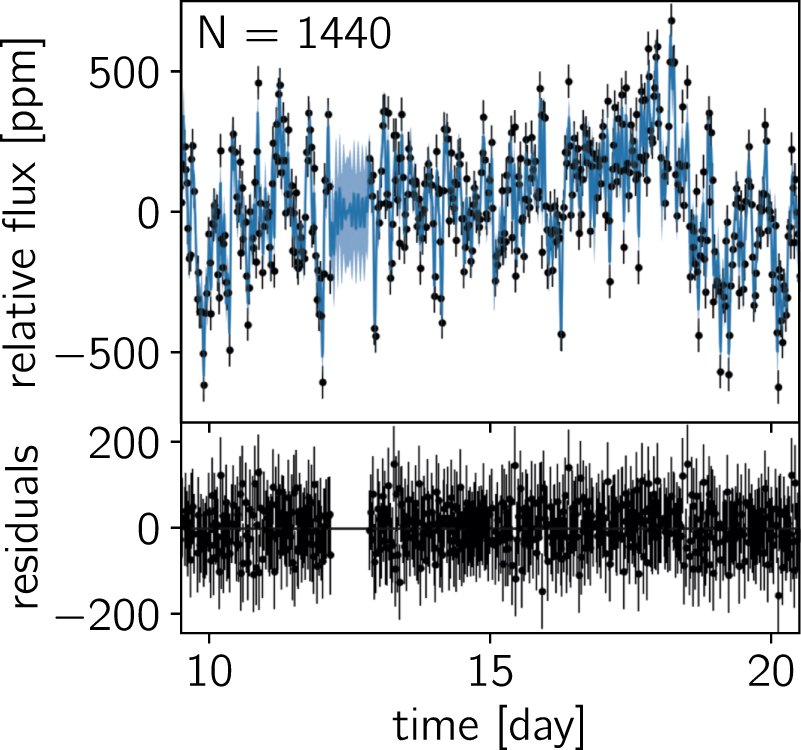
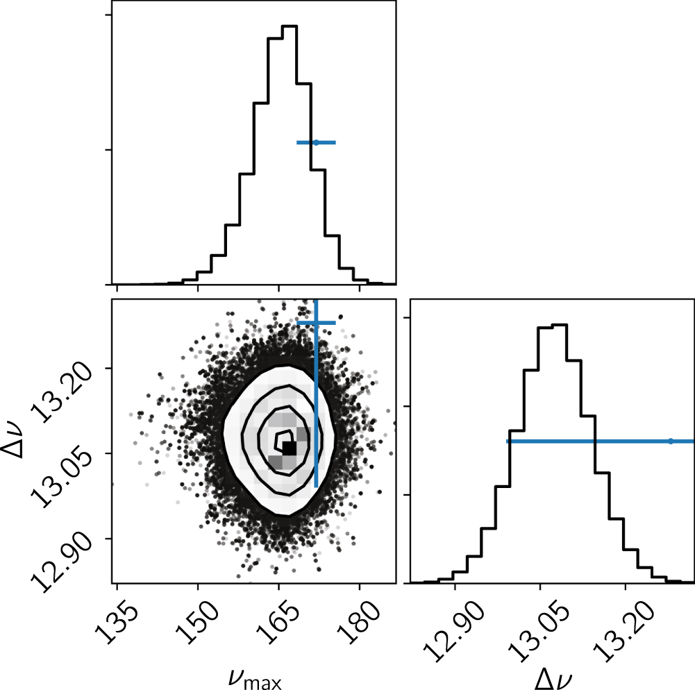
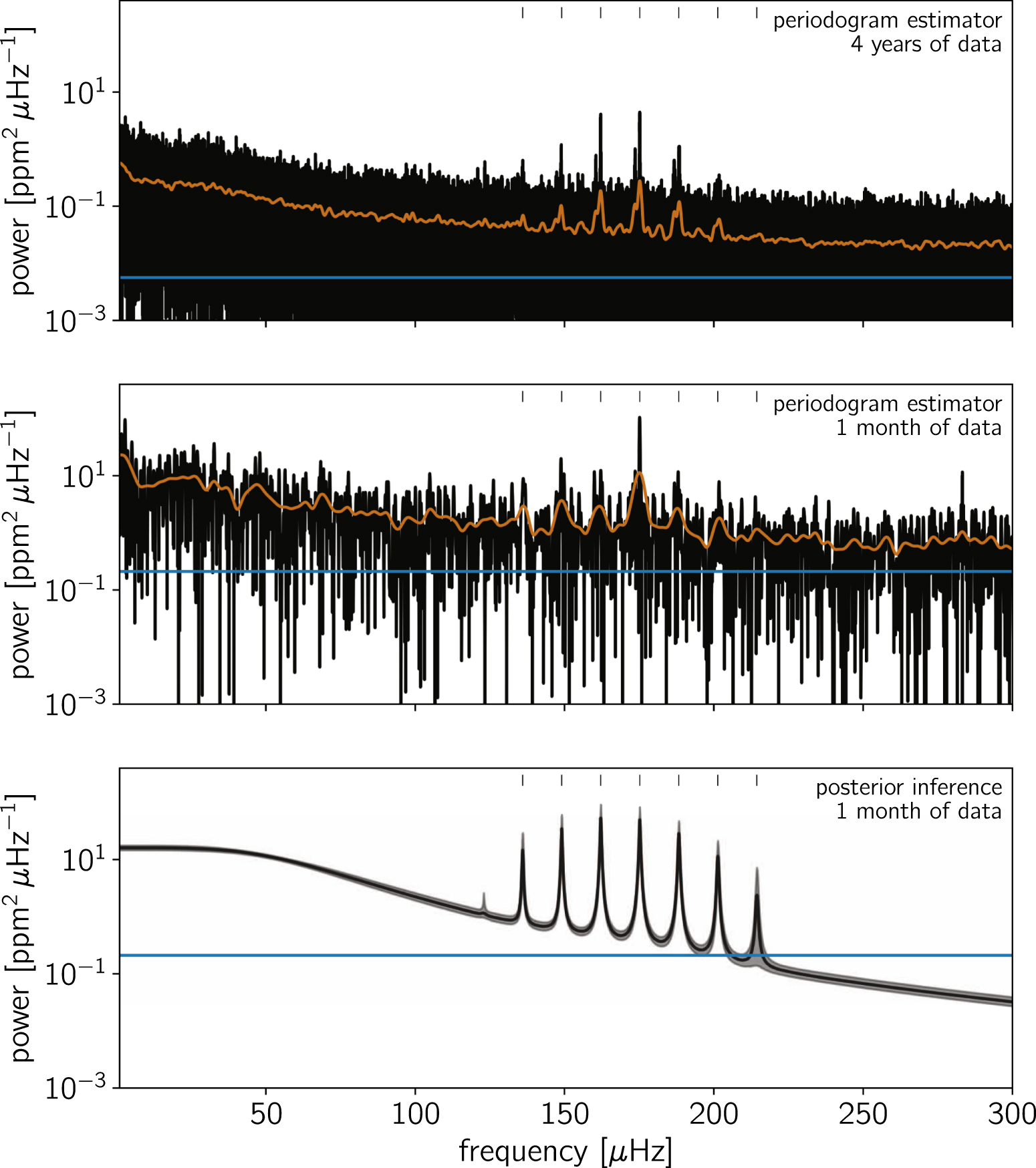
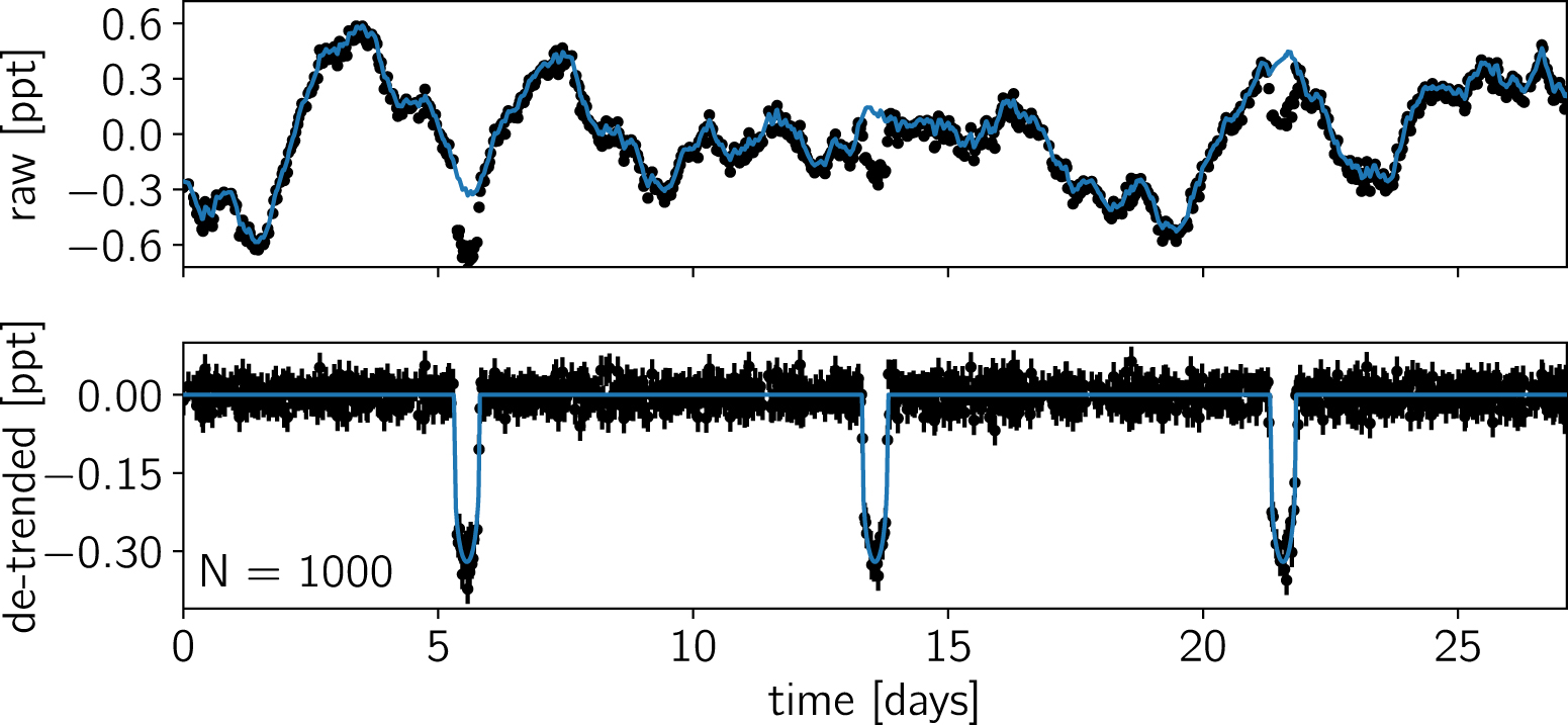
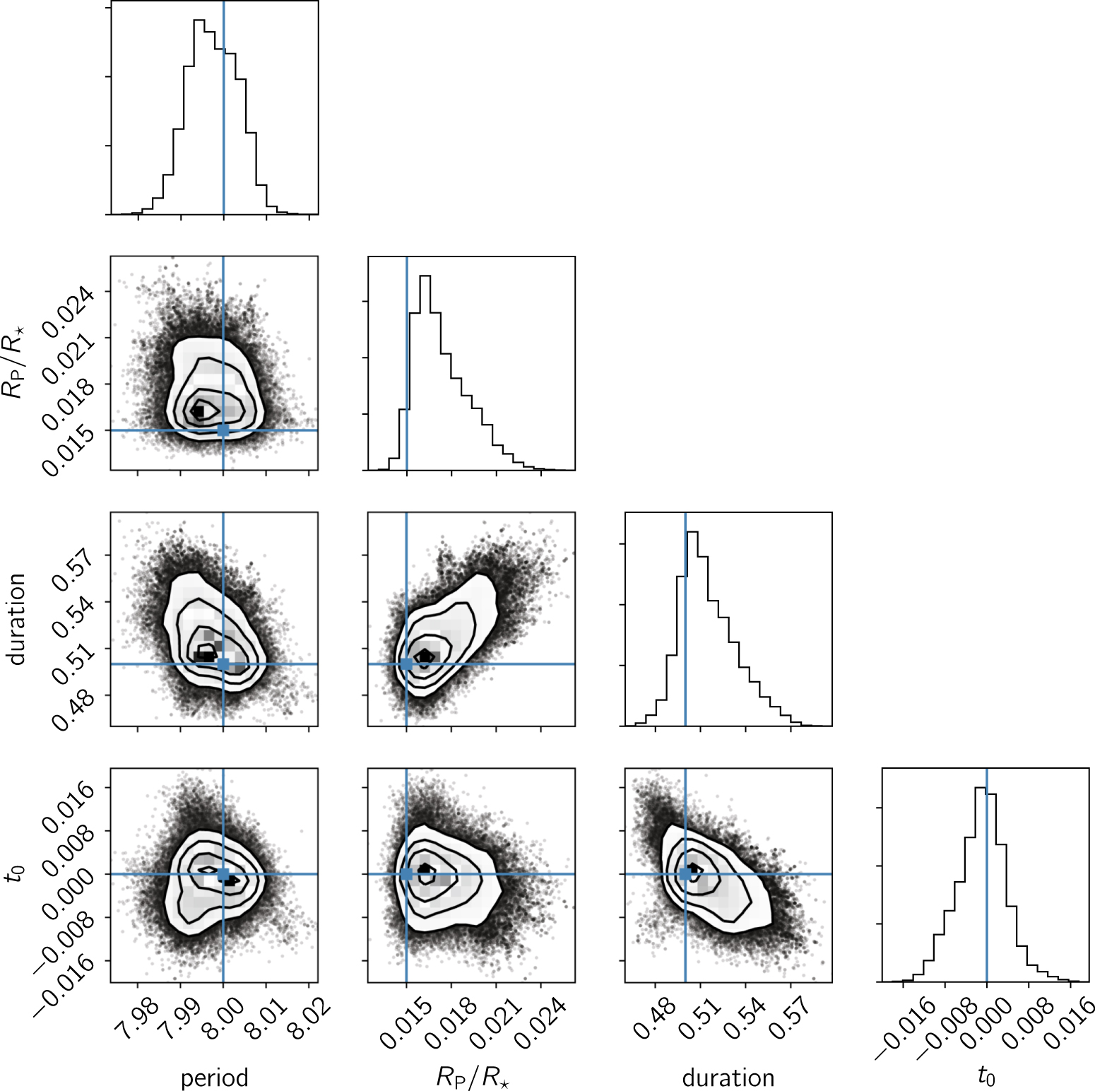