
Abstract
Improvements in synchrotron based operando X-ray tomographic microscopy (XTM) of polymer electrolyte fuel cells (PEFCs) have paved the way for 4D imaging studies of the water distribution in the gas diffusion layer (GDL). In order to capture the full water dynamics in 4D, a decrease of the scan time towards 0.1 s is aspired, posing significant challenges in image processing for quantitative water detection. In this work, ex situ and in situ X-ray tomographic microscopy experiments were conducted to study the influence of imaging parameters and image denoising settings on image quality and water detectability in the GDL. The image quality is quantified for scan times between 50 ms and 12.8 s at the TOMCAT beamline of the Swiss Light Source. Denoising strategies for a broad range of image qualities were identified, which enable high in situ water detectability rate of 96% at a scan time of 1.6 s and 88% at subsecond scan time as short as 0.4 s. The presented methodology can be transferred to other PEFC or similar XTM imaging setups and image processing pipelines to verify their water detection capabilities.
Export citation and abstract BibTeX RIS

This is an open access article distributed under the terms of the Creative Commons Attribution Non-Commercial No Derivatives 4.0 License (CC BY-NC-ND, http://creativecommons.org/licenses/by-nc-nd/4.0/), which permits non-commercial reuse, distribution, and reproduction in any medium, provided the original work is not changed in any way and is properly cited. For permission for commercial reuse, please email: permissions@ioppublishing.org.
Polymer electrolyte fuel cells (PEFCs) convert chemical energy stored in hydrogen to electricity.1 Due to their relatively high conversion efficiency and high power density, PEFC technology is considered as a power source for mobile, stationary and aerospace applications.2–5 In the electrochemical reaction, water is generated at the cathode catalyst layer. At high power densities and/or low temperature operation, product water removal via gas phase is not sufficient, such that the pores of the catalyst and gas diffusion layers (GDLs) become partially filled or completely flooded with liquid water. GDLs are thin, carbon fiber based, highly porous materials with the typical average pore sizes in the range of 18 μm to 35 μm6 and large pores in some materials reaching diameters of up to 200 μm,7 providing gas diffusion pathways from the gas feed channels to the catalyst layers. Condensed water in the GDL pores limits the reactant gas transport, lowering cell performance and efficiency. Appropriate water management in the GDL is therefore critical to ensure adequate gas transport and product water removal.8–10 In order to understand the structure-property-relationships of liquid water in GDLs, operando imaging techniques utilizing neutron and X-ray sources, to penetrate the opaque cell materials have proven successful tools for the characterization of the liquid water distribution in PEFCs.
Radiography images can provide insights into the water distribution in GDLs,11–16 however, the 2D radiography images provide only averaged projections of the water distribution along the beam direction, which makes it difficult to analyze individual pores and water clusters. Therefore, X-ray tomographic microscopy (XTM) has been increasingly utilized in the past decade as a 3D characterization technique, enabling studies of the liquid water distribution in GDLs with a spatial resolution in the micrometer range.17–28 Most studies have been performed at synchrotron sources, that can also provide adequate temporal resolution. Eller et al. reported 4 min scan times with a voxel size of 1.85 μm for progress in operando imaging studies in 2011.18 Zenyuk et al. employed XTM scan times of 30 s with a voxel size of 2.5 μm to study evaporation in GDLs in 2016.19 In 2017, Eller et al. further developed operando XTM setups for investigating GDL saturation and liquid permeability with XTM scan times of 10 s and a voxel size of 2.9 μm.26 In 2019, Nagai et al. reported about improved water management through microporous layer modifications that was verified via operando XTM with just 1.6 s scan time at a voxel size of 3 μm.28 These advancements in XTM setups and image processing have paved the way for 4D operando imaging studies of the non-steady water distribution in GDLs.
Because the transient behavior of water in the GDLs has characteristic time scales in the range of a few milliseconds to minutes,29,30 it is indispensable to advance the temporal resolution of XTM to gain a better understanding of the fast underlying processes. However, to achieve XTM scan times of less than a second, some technical limitations need to be overcome. Firstly, high brilliance synchrotron X-rays, together with highly efficient microscopes and fast CMOS-based cameras are required to collect radiographic projections within about a millisecond or less. Secondly, complex operando PEFC setups need to be developed compatible with the fast rotation speed. Thirdly, an optimized image processing pipeline, which efficiently implements image denoising, image segmentation and image evaluation is necessary to provide precise, quantitative information from the fast XTM scans. Finally, a careful analysis of the consequences of the aspired subsecond XTM imaging, on the image quality and water detectability is vitally important to verify the advancements.
In this work, ex situ XTM experiments with liquid water filled flow field channels and in situ experiments with electrochemically generated water, but not operating cells, are conducted to study the influence of scan times between 0.4 s and 12.8 s on the image quality and consequences on the water detectability. A contrast-to-noise ratio (CNR)31 analysis is employed to quantify the image quality at the different imaging conditions, including variations of the monochromatic beam energy, the number of projections as well as the exposure time per projection. Furthermore, the influence of image denoising during the segmentation workflow on the detectability of artificial (ex situ based) and in situ generated microstructural water features will be discussed. The influence of the image denoising filter combinations are identified by a surface identification analysis. Finally, scan time dependent optimal denoising filter combinations are identified and verified by a water detectability analysis.
Experimental
Materials and setups
PEFC & materials
An imaging PEFC with an active area of 0.16 cm2 (4.5 mm × 3.6 mm), designed by Eller et al.,26 was used for the XTM imaging experiments (see Fig. 1a). The flow field plates were made of graphitic material (BMA5, SGL Technologies) and have two channels for both anode and cathode with a width of 0.8 mm and a depth of 0.3 mm. The cell temperature was monitored and regulated during the XTM imaging experiments by PT100 temperature sensors and heating foils inserted in the cell assembly. A catalyst coated membrane (CCM) from W. L. Gore & Associates (Gore® Primea® A510.1/M815.15/C510.4 with a 15 μm thick reinforced Gore-Select® membrane and anode/cathode Pt loadings of 0.1/0.4 mg cm−2)32 together with plain Toray TGPH-060 carbon fiber (Toray Industries Inc.; 0% hydrophobic coating; no microporous layer; through-plane and in-plane average pore diameter of 29 μm and 49 μm7 respectively) as anode and cathode gas diffusion layers were used.

Figure 1. (a) Schematic of a specially designed double channel fuel cell for XTM imaging; (b) experimental setup at TOMCAT beamline for the ex situ water experiment and (c) for the in situ water experiment; (d) schematic of the cell components in through-plane view; (e) tomographic through-plane slices obtained for the ex situ experiment showing the purposely water filled cathode flow field channels and (f) the in situ experiment showing water accumulations in frozen state in the flow field channels when cell was cooled to −20 °C after operation.
Download figure:
Standard image High-resolution imageEx situ experiment
The cathode flow field channels were filled with liquid water after cell assembly to establish a well-defined liquid water filled volume for statistical analysis of the XTM gray scale values (see Fig. 1e). The ends of the flow field capillaries were sealed with silicone tubes to prevent water loss during the XTM imaging (see Fig. 1b; silicone tubes not shown).
In situ experiment
A PEFC was operated at 0.5 A cm−2 with H2/air (100%/100% relative humidity) at 25 °C for 30 min to generate a realistic water saturation in the GDLs. Then the cell was stopped, gas supply and cell heating were switched off and cell outlets were sealed with silicone tubes. The electrochemically generated water distribution was immobilized and kept in a steady state during the XTM imaging by cooling the cell below −20 °C with a freezing device developed by Mayrhuber et al.21 (see Fig. 1c). The freezing device made use of a 3D printed freezing chamber that is equipped with Kapton foil windows to achieve nearly attenuation-free X-ray transmission and unbiased XTM image quality.
Synchrotron X-ray tomographic microscopy
Synchrotron based X-ray tomographic microscopy (XTM) experiments were implemented at the TOMCAT (X02DA) beamline of the Swiss Light Source (SLS) at the Paul Scherrer Institut (PSI) in Switzerland. A Ru/C multilayer monochromator (ΔE/E ∼2%–3%) was used to select monochromatic X-ray radiation at several different energies (11 keV, 13.5 keV, 16 keV, 18.5 keV). The radiography images were collected by the GigaFRoST camera system,33 coupled with a 2–4× microscope (Elya Solutions, Czech Republic) equipped with a 100 μm thick LuAG:Ce scintillator. The magnification was set to 3.48 resulting in 3 μm voxel edge length. The XTM scan time is calculated by the multiplication of the exposure time per radiography (0.5 ms to 16 ms) and the number of projections (25 to 1600) per scan over 180° resulting in a scan time range of 0.05 s–25.6 s where the shortest achievable scan times were limited by the stage maximum rotation speed of 10 Hz. The camera readout was cropped to 2016 px (horizontal) × 700 px (vertical) to avoid camera readout time limitations for all exposure times. 3D XTM absorption contrast reconstructions were obtained from the collected radiographic projections through Gridrec reconstruction algorithm.34
Methodology & Image Processing
Contrast-to-noise ratio
In order to quantify the influence of the imaging conditions and beam energies on the image quality, the contrast-to-noise ratio (CNR) was evaluated comparing gray scale values of bulk water in the liquid filled cathode flow field channels and an empty anode flow field channel (void domain) as an indicator of how well water and void domains can be distinguished in the GDL:
The mean and standard deviation (Std) of the gray scale value (GSV) of the water filled and void channel domains were calculated for a total of 4.7 × 10⁷ voxels, by concatenating 5 different cuboid subvolumes (174 × 54 × 100 voxels) that were extracted from the tomographic dataset at different positions along the channel direction.
Denoising and segmentation
The 3D gray scale value (GSV) voxel data is obtained after reconstruction from the radiographies. The water signal provides higher GSVs than void but similar to the GDL fibers' GSVs, which causes difficulties in histogram-based segmentation. Thus a reference scan of the cell in dry state was obtained at the end of the experiments to subtract all the static dry structures from the scans of the operating cells to isolate the water signal. Careful alignment of wet scans to a reference dry scan is necessary to get precise segmentation of the correct water signal. The general denoising and segmentation pipeline is given in Fig. 2b. Both dry and wet scans were filtered with a 3D median filter (kernel radius size in pixel, denoted as M[1] for kernel radius of 1 px) to reduce image noise before subtraction. The resulting difference images were further filtered with an anisotropic diffusion filter (AD, denoted as AD[1] for iteration of 1),35 known as edge-preserving filter, to enhance the water signal and prevent edge shifting due to intensive median filtering. There exist also alternative image denoising filters that are not discussed in this work, i.e. Garcia-Salaberri et al.36 used 3D bilateral filter, Heenan et al.37 applied a non-local means filter and Kaestner et al.38 applied a regularized inverse scale space filter. A threshold value was then chosen and applied to obtain binary segmented water mask to which an additional 3D hole closing for filling small voids in the bulk water structure and a cluster cleaning for background noise removal were applied. In parallel, the dry scan was segmented to obtain the GDL fiber structure only. The pore structures in GDLs were obtained by inverting the binary segmented GDL fiber structure. The water mask and the solid fiber mask were merged in the end to obtain the final three phase segmented images for further quantification.
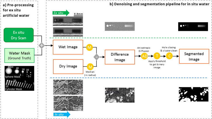
Figure 2. Image denoising and segmentation pipeline for (a) the ex situ artificial water structure based experiment and (b) the electrochemically generated in situ water experiment.
Download figure:
Standard image High-resolution imageGround truth reference state preparation
The precise quantification of the water detection capabilities for the different XTM scan settings requires a reference state of the water distribution in the sample, called ground truth (GT). Considering the fact that the liquid water in the GDLs does not remain static over a long term observation period during an operando XTM experiment,39 referencing operando liquid water by an operando ground truth seems impossible. Therefore, two alternative approaches were employed to obtain a water ground truth based on artificial and in situ water structures, respectively.
The artificial water structures approach in this work is similar to the work presented by Kaestner et al. on XTM of 3D root networks.40 In this work, XTM data is simulated by adding background noise from XTM scans acquired with different imaging conditions to ground truth structures, instead of adding artificial noise to the ground truth structures as done in.40 The water feature ground truth mask contains 3D structures simulating water accumulations in individual pores as spheres with diameter sizes in pixels of (60, 40, 20, 10, 9, 8, 7, 6, 5, 4, 3, 2, 1) and water accumulations in the throats connecting different pores to larger clusters as columns with diameter sizes in pixels of (13, 12, 11, 10, 9, 8, 7, 6, 5, 4, 3, 2, 1) as shown in the 3D rendering in Fig. 2a. The ground truth binary structures are then multiplied with a value that represents mean GSV difference between water and void domain based on CNR analysis. Finally the ground truth structures are added to the empty channel positions in ex situ XTM scans to simulate the water structures in real scans as shown in Fig. 2b.
For the in situ water structures, the electrochemically generated water was immobilized by freezing throughout the in situ XTM imaging period. The ground truth image was obtained by following the same filtering and segmentation workflow as detailed in Fig. 2b on a high quality XTM scan with 25.6 s scan time and only very mild image denoising by anisotropic diffusion filter (AD[1]).
Verification of surface identification
The filtering processes applied during image denoising and the threshold selection during segmentation may influence the shape and the surface of the segmented water structures and therefore alter the overall detected total water volume. A shell-wise analysis of the near surface voxel layers within and outside the artificial water structures is used to investigate the accuracy of the surface identification. The quantification approach by surface identification uses a layer by layer (step of 1 voxel) decomposed shell structure of the ground truth as reference. For instance, for one of the ground truth water droplets (e.g. diameter of 20 voxels), the voxels belonging to the shell between the surface [0] and the inside [−1] position were defined as ground truth for the surface [0] position. The range of shells was selected from inside the object [−5] to the outside [+5]. Hence, for each scan the voxels belonging to a shell layer in a segmented image are counted and then divided by the number of voxels in the same shell of the ground truth to obtain the surface identification value in percentage. The analysis was applied at three independent positions in each XTM scan for same artificial water structures and the individual surface identification values were averaged to reduce statistical errors.
Water detectability
To characterize the image denoising and the segmentation workflow, the water detectability (WD) has been defined as a selection criteria for exploring suitable image filtering parameters. Through the denoising and segmentation workflow in Fig. 2b, a binary segmented image can be obtained and compared voxel by voxel with the pre-defined ground truth—a 3D water feature mask in case of the ex situ water experiment and a segmented high quality 3D mask in case of the in situ water experiment. The percentage of correctly water labeled voxels is defined as the 3D water detectability value. The percentage of incorrectly water labeled voxels in a shell of 10 voxels extending from the surface of the ex situ ground truth water is defined as the false water in the surrounding background. The evaluation was applied at five independent positions in each XTM scan and the calculated water detectability values were averaged to avoid fluctuations due to random sampling errors. For the artificial water case, it is possible to breakdown the water detectability assessment for each different sphere and column sizes to obtain feature based water detectabilities. For the segmented high-quality mask, the water detectability is defined and calculated considering the complete ground truth structures. The analyzed subdomain cuboid used for the evaluation of the in situ data was located under the channel in the cathode GDL with a dimension of 720 μm × 720 μm × 30 μm.
Terminology
A summary of abbreviations used in this paper is listed in Table I.
Table I. List of abbreviations.
| Abbreviation | Meaning |
|---|---|
| XTM | X-ray tomographic microscopy |
| PEFC | polymer electrolyte fuel cell |
| GDL | gas diffusion layer |
| CNR | contrast-to-noise ratio |
| CCM | catalyst coated membrane |
| M[1] | median filter with kernel radius of 1 px |
| AD[1] | anisotropic diffusion filter with 1 iteration |
| GT | ground truth |
| BG | background |
| GSV | gray scale value |
| WD | water detectability |
| AS5 | artificial sphere with diameter of 5 px |
| AC5 | artificial column with diameter of 5 px |
| PSI | Paul Scherrer Institut |
| SLS | Swiss Light Source |
Results and Discussion
Evaluation of image quality
Short tomographic scan times in the subsecond regime, which are necessary for studying water dynamics in GDLs will have inherently low image quality. In order to obtain best results at a given scan time, it is vital to understand the influence of the imaging conditions on the image quality. At first the influence of the beam energy, the radiography exposure time and the number of projections on the image quality is studied for the pure, bulk domains of the different phases in the cell's flow field channel domains (ex situ data). In a second step the sensitivity of the water surface location on threshold selection and image filtering is analyzed for artificial water structures. Finally the gained knowhow is applied to "real," in situ electrochemically produced water structures. These in situ measurements were performed at −20 °C to perfectly conserve the same water structure for all imaging conditions.
The CNR between liquid water and void domains as defined in Eq. 1 was studied for 4 monochromatic beam energies (11, 13.5, 16, and 18.5 keV) with tomographic scan times ranging from 0.05 to 25.6 s. For the chosen image dimensions, bounded by the sample size, the 0.05 s scan time was the fastest achievable acquisition speed supported by the hardware of the TOMCAT beamline. The effect of the scan time variation on image quality at 13.5 keV is shown in Fig. 3 for the full combination of exposure times (0.5–16 ms) and number of projections (25–800). While the empty flow field channels remain visible down to a scan time of 0.05 s in the through-plane slices, the GDL structure can be only seen until 0.8 s scan time, suffering though from significant detail losses. The general trend of the image quality losses with shorter scan times can be expected41–43 and is quantitatively described by the CNR values stated for each tomographic slice in Fig. 3 by yellow numbers.

Figure 3. Through-plane tomographic slices obtained for the full combination matrix of exposure time and number of projections for ex situ water experiment; contrast-to-noise (CNR) ratio values calculated between water and void domains (indicated as yellow dashed areas in 12.8 s XTM scan) are presented in yellow font for each slice.
Download figure:
Standard image High-resolution imageThe CNR values at the same scan times are similar, with slightly lower values for shorter exposure times, especially for exposure times below 2 ms, where also more ring artefacts are observed. Scans settings with 100 projections or less show well visible under-sampling artifacts in the form of stripes especially at the edge of the XTM through-plane slices. Therefore, all analysis steps beyond noise and CNR analysis are limited to scan conditions with ≥200 projections and ≥2 ms exposure times.
The influence of the beam energy on image contrast is shown in Fig. 4a. At an energy of 13.5 keV the CNR values are the highest for all scan times, though 16 keV shows very similar values. At the lowest energy of 11 keV, the X-ray flux at the beamline is the lowest and therefore the CNR values are the lowest. The reduction of the CNR values for 18 keV is due to the decrease of the attenuation coefficient of water at higher energies. It is important to note, that the energy dependency of the CNR value remains beamline specific when referencing to scan time, as the spectral distribution of the X-ray photon flux and the energy dependency of the detection system are beamline specific. A detailed analysis of the contributions of mean and standard deviation levels to the CNR at 13.5 keV is shown in Fig. 4b. The mean GSV of both H2O and void domains remain stable with varying scan time, as the beam energy related attenuation coefficients are not affected by the scan time. The standard deviations increase with decreasing scan time as expected,41–43 especially for subsecond scan times, reaching similar values for the water and void domains. When the scan time is reduced to 0.4 s or lower, the standard deviations of the background noise are almost the same as the mean GSV level of the H2O domain, and with the noise level reaching the signal level, the CNR drops to 1 and below. In Fig. 4c, the square of the CNR value is plotted vs scan time to enable a linear fitting as the shot noise is proportional to the square root of the number of photons on the detector.44 A coefficient α is introduced to fit the linear relationship for different XTM exposure times (see Fig. 4c). The coefficients of α for 0.5 ms and 16 ms exposure time define a lower and upper boundary conditions for the CNR values for different scan times. This enables the prediction of image quality in terms of CNR for untested combinations of scanning conditions. The CNR value range is given by the following Eq. 2:

These values correspond to the yellow domain in Fig. 4c.

Figure 4. (a) Contrast-to-noise ratio (CNR) between water and void domains for different tomographic scan times at beam energies between 11 keV and 18.5 keV; (b) mean and standard deviation of the water and void domains GSV vs scan time at 13.5 keV; (c) square of CNR(H2O/Void) values vs scan times with linear fitting with formula CNR2 = α * T for different XTM exposure times at 13.5 keV; α is defined as a linear coefficient and T is the scan time in seconds; the yellow marked area indicates the range of possible CNR values for scan times between 0.05 s and 12.8 s (see Eq. 2).
Download figure:
Standard image High-resolution imageChoice of segmentation threshold
Threshold based segmentation is the simplest image processing approach to extract quantitative information from XTM scans. To evaluate the influence of denoising filter combinations on water detectability, a choice of the segmentation threshold needs to be made beforehand. Based on the detailed CNR analysis shown above, a threshold value at 50% of the difference between the GSVs of water and the background in the difference image was selected as the water threshold value.
The surface identification method was applied exemplarily to the artificial water sphere with a diameter of 20 px to show the sensitivity of the threshold selection on the segmentation result. In Fig. 5, the influence of threshold variations between 42.5% and 57.5%, where the mean GSV of the water signal corresponds to 100% and background signal to 0%, on identification of the water surface is presented. The selection of a too high threshold value (over-thresholding: >50%) reduces the false water detected beyond the spheres surface but results also in a loss of water volume detected within two or more layers underneath the sphere's surface, hence lowering the overall water detectability. On the other hand, a too small threshold value (under-thresholding: <50%) provides a higher amount of water closer to the shape edge profile of the ground truth, but the falsely identified water outside the original spherical domains increased as well. For the underlying noisy background of the 1.6 s scan time dataset used in this example, some errors in water detection will always remain, even after denoising.
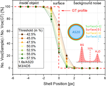
Figure 5. Influence of threshold variation on the surface identification value for an artificial water sphere structure with a diameter of 20 px in a filtered (M[3]+AD[5]) 1.6 s ex situ water scan. Shell position is varied from [−5] to [+5] with the surface denoted as [0]. The ideal ground truth (GT) profile is indicated as a red dashed line.
Download figure:
Standard image High-resolution imageSurface sensitivity to denoising
XTM scans with low CNR require appropriate image denoising prior to segmentation in order to increase the detection level of correctly labeled water domains and to minimize the amount of falsely assigned water domains. Median and anisotropic diffusion (AD) filters were chosen to reduce the noise in the data while preserving the edges of the water boundaries. In Fig. 6, the surface identification of all tested combinations of the median and AD filters are presented to demonstrate the influence of image denoising on the surface of selected features (artificial spheres with diameter of 5, 10, and 20 px; denoted as AS5, AS10, and AS20) for segmented images of the 1.6 s scan time dataset.
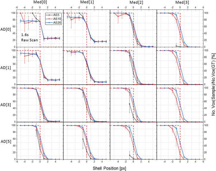
Figure 6. Influence of image filtering combinations on surface identification values based on a 1.6 s ex situ water scan with 50% threshold for segmentation. The error bars were derived from the averaged surface identification values at 3 different sampling positions.
Download figure:
Standard image High-resolution imageIn the unfiltered raw reconstruction, the background noise level is higher than 20% and the signal level is below 80%. Median and AD filters are both able to reduce the background noise down to below 5% and improve the water detection level of the inner bulk layers [−4, −5] up to 100%, when being applied individually with a radius of 3 (Median) or 5 iterations (AD). However, strong median filtering (e.g. M[3]) deteriorates the surface [0] and the inner layers [−1, −2] and decreases water detection levels compared to higher iterations of the AD filtering (e.g. AD[5]) for the larger spheres AS10 and AS20. The small sphere AS5 disappears almost completely by the median filtering with radius 3, but is better preserved, though not 100%, by the AD filtering with 5 iterations. Thus there is a limitation for employing strong median filtering for the denoising of datasets where small features need to be identified. Combinations of mild median and AD denoising are therefore beneficial to ensure a correct surface representation and the detection of small features, as i.e. for M[1]+AD[3] in this example.
Feature based water detectability
The influence of the denoising filter combination was studied not just for the 1.6 s scan time but for a broad range of scan times. Figure 7 presents the quantification of the feature based water detectability (WD) of artificial spheres (AS5, AS10, AS20) and columns (AC5, AC10, AC20) for selected scan times. The WD values for all selected feature sizes decrease from nearly 100% at a scan time of 12.8 s to below 70% at 0.4 s and the background false detection rates increase accordingly from below 5% at 12.8 s up to nearly 40% at 0.4 s for the unfiltered raw data (see Fig. 7a). In general, the column structures were found less sensitive towards filtering in terms of WD than sphere structures, due to their higher connectivity. For realistic operando scans it means that the connected water clusters spanning over several pores will be better preserved than isolated droplets of a similar diameter.
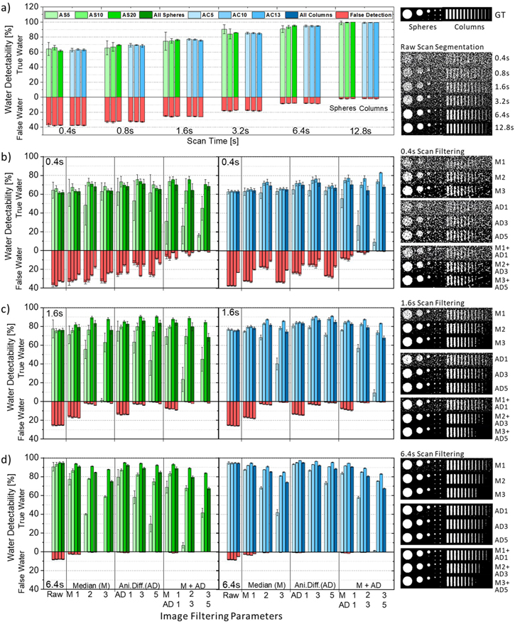
Figure 7. Water detectability analysis based on selected simulated features of artificial spheres (5, 10, 20 px diameter; green bars) and columns (5, 10, 20 px diameter and 60 px height; blue bars) for (a) raw scans with scan times from 12.8 s to 0.4 s; (b) 0.4 s scan; (c) 1.6 s scan; (d) 6.4 s scan. Image filtering combinations are denoted at the bottom as raw/no filtering, 3D median (M) filtering of 1, 2, 3 (kernel radius size in pixel), anisotropic diffusion (AD) filtering with 1, 3, 5 iterations and combinations of median and AD filtering. The error bars were derived from the averaged water detectability values at 5 different sampling positions. The corresponding 2D representations of 3D segmented slices are shown on the right for visual explanation of filtering effects. Ground truth of water features is shown at the top right.
Download figure:
Standard image High-resolution imageThe influence of the filter combination on the WD values are presented for the selected scan times of 0.4 s, 1.6 s and 6.4 s. For a fast 0.4 s scan a strong filtering combination (M[3]+AD[5]) is required to obtain a clean background at the cost of losing any small features below 5 px (see Fig. 7b). By doing so the overall WD values for all sphere and column features are approximately 70%. Whereas, for a 1.6 s scan (see Fig. 7c), a less aggressive filter combination (M[2]+AD[3]) is appropriate to suppress background noise while keeping the detectability ratio high even for small sphere (AS5) and column(AC5) features. At the scan time of 6.4 s already mild filtering of AD[1] is sufficient to get rid of the minor background noise. The water structures are not significantly affected by the mild filtering itself, reaching a high overall WD level of around 90% (see Fig. 7d).
In situ water detectability
The influence of the image filtering quantified for surface identification and water detectability discussed above for the artificial water structures, remains to be verified for in situ water structures with electrochemically produced water. To maintain the in situ water structure stable for all combinations of scan settings, the water was immobilized by freezing the cell to −20 °C. Water detectability (WD) results for representative scan times of 0.4 s, 1.6 s, 6.4 s and selected filtering combinations are presented in Fig. 8.
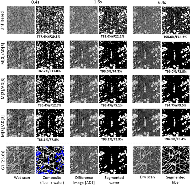
Figure 8. Water detectability analysis for in situ generated water. Selected scan times (0.4 s, 1.6 s, 6.4 s) and 4 image filtering combinations (unfiltered; M[0]/AD[5]; M[2]/AD[3]; M[3]/AD[5]) are shown in a matrix with the left figure representing the difference image between a wet scan and dry scan and the right figure the corresponding segmented image. Water detectability values are indicated below the segmented image as true (T) and false (F) water in %. At the bottom the high quality 25.6 s scan considered to be the ground truth is presented. From bottom left to right: the 25.6 s wet scan, composite of fiber (white) and water (blue overlay) segmentation, difference image between a wet and dry scan with slight filtering of AD[1], segmented water based on the filtered difference image, 25.6 s dry scan and segmented fiber structure based on the dry scan.
Download figure:
Standard image High-resolution imageFor the unfiltered, raw reconstructed XTM data, similar water detection levels as for the artificial datasets were found with correctly detected true water levels ranging from 78% to 96%, for 0.4 s to 6.4 s scan time, respectively. For a fast scan of 0.4 s, a strong filtering combination (M[3]+AD[5]) is required to reduce the background noise from 29% to only 8% and thereby increasing the true water detection level to almost 90%. Similarly, also for the scan time of 1.6 s, substantial image denoising is needed to reduce false water detection rates to 4%–5%, whereas the selected filter combinations have only minor influence on the true water detection rates at 93%. For a scan of 6.4 s, filtering of AD[5] is sufficient to suppress the background noise, while strong filtering does even slightly decrease the water detection level from 96% to 94% as contours are blurred and fine details are lost. Similar high water detection levels were reported recently by Xu et al.45 for subsecond scans using a high magnification microscope (0.4 μm voxel edge length) and high intensity polychromatic beam conditions at the TOMCAT beamline. Since the density of ice is about 8.3% lower than that of liquid water at 0 °C,46 the reported water detectability values can be considered as conservative, slightly underestimating the water detectability levels for GDLs containing liquid water.
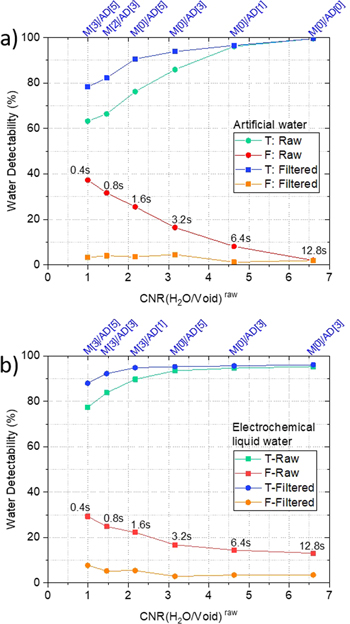
A summary of the achievable water detectability levels for both the artificial and in situ water structures applying scan time specific image denoising is shown in Fig. 9. The selected filtering combinations are able to maximize the water detectability for various scan times. For a raw reconstructed scan with a CNR value of 1, a water detectability of nearly 90% is achieved after filtering, with false detection rate remaining below 10%. In case of the unfiltered raw conditions, the artificial water detectability is found underestimated for fast scans and overestimated for longer scans when compared to the in situ data. When image denoising filters are applied, the artificial and in situ water detectability analysis show similar trends with a maximum deviation of the true water detection levels at about 10%. The underestimation of the ex situ water detectability at short scan times is probably due to edge enhancement effects of the coherent X-ray beam in the absorption contrast in situ data. The edge enhancement, supposedly reducing edge blurring, especially with anisotropic diffusion filtering, is not included in the artificial water structures. Whereas the reduced in situ detectability at a long scan time of 12.8 s is probably caused by minor registration errors between the wet scans and the dry reference scan that are not present in the artificial data, since no image registration is needed for the artificial data.
Figure 9. Water detectability vs contrast-to-noise ratio (CNR) between water and void of XTM scans for (a) the ex situexperiment (artificial water) and (b) the in situ experiment (electrochemical water). Raw and filtered water detectability results in terms of correctly detected water in ground truth (T) and falsely labelled water in the background (F) are shown for selected best filtering combinations for each scan time from 0.4 s to 12.8 s.
Download figure:
Standard image High-resolution image
Since the water detection levels are presented relative to the CNR values of the corresponding scan times in Fig. 9, it could be possible to compare and transfer findings of this work to other fuel cell XTM imaging setups, independent if in situ frozen water detectability experiments are possible or not. Therefore, it provides guidelines for the selection of the imaging conditions, depending on the required precision of XTM quantitative analysis.
Conclusions
The influence of image acquisition conditions and image denoising on the quality of XTM scans and the liquid water detectability in GDLs of PEFC was studied at the TOMCAT beamline of the Swiss Light Source (SLS). The image quality was quantified by evaluating the contrast-to-noise ratio (CNR) between water and void domains for different scan times and beam energies. For beam energies ranging from 11 keV to 18.5 keV and tomographic scan times varying from 0.1 s to 12.8 s, the CNR value was found the highest for the beam energy of 13.5 keV. At this energy, the image quality is limited by the artifacts induced by either very short exposure time (<2 ms) or an insufficient number of projections (<200). The CNR value drops from 6.6 (at 12.8 s scan time) to less than 1.5 for scan times shorter than 1 s, reaching a minimum of 0.5 for a scan time of 0.1 s at 13.5 keV. While the mean gray scale values (GSVs) of the water and the void domains remain constant with scan time at a given beam energy, the standard deviation is growing with shorter scan times and hence drives the decrease of the CNR to lower values.
The detectability of the liquid water in the GDLs was quantified by comparing the segmentation results of two types of water in the images. Artificially introduced water features (spheres and columns of different size) and electrochemically created in situ liquid water structures were analyzed for different scan times and compared to a ground truth reference. The low CNR values of the fast XTM scans require appropriate image denoising prior to segmentation which implies a compromise between the detection of small water features and the reduction of falsely detected water in the background. The segmented water features were found to be more effected by the median filter than by the anisotropic diffusion filter and individual best filter combinations were identified for the different scan times. Only a mild filtering is needed for scans with high CNR values, while strong denoising is necessary for scans that have low CNR values. The detectability level of the artificial water structures reached nearly 100% for a high quality unfiltered scan of 12.8 s with a CNR value of 6.6 and remained above 90% after adequate image denoising when the scan time was reduced to 1.6 s (CNR = 2.2). Similar water detection levels were observed for the in situ water structures, though they did not exceed 97% even at the 12.8 s scan time, likely, due to minor dry registration errors between the dry and wet scans. The water detection rate remained above 90% for scan times down to 0.8 s (CNR = 1.5) as the in situ water structures are better connected than the isolated artificial spheres and column structures.
The presented methodology can be used to verify the achievable water detection levels of other PEFC or similar XTM imaging setups, with the ex situ artificial water approach being easily transferable, whereas the in situ ground truth comparison requires the availability of an XTM compatible freezing setup. By referencing the water detectability levels to the CNR values of the bulk liquid water and void domains of the XTM data, the analysis is decoupled from the instrumentation specific scan times. This generic representation may allow to compare the findings with other fuel cell XTM imaging setups in the community independent of scan time but related to image quality. The presented detection levels could be used as an estimate for the liquid water detection rates when only CNR data but no ground truth is available, or as a benchmark for image processing pipelines, when ground truth data is available.
In the future, it is expected that operando subsecond X-ray tomographic microscopy of PEFCs with proven liquid water detection rates will further advance as a tool to understand transient water transport phenomena and their influence on PEFC performance. Exploiting new beamline instrumentation,42 alternative contrast options such as propagation-based phase retrieval or iterative reconstructions schemes are feasible to push the achievable scan rates for these investigations to 10 Hz and even beyond to 20 Hz at the TOMCAT beamline of SLS.
Acknowledgments
Financial support from the Swiss National Science Foundation (SNF) under grant No. 200021 166064, software and electronic support by T. Gloor, as well as support during measuring campaigns at the TOMCAT beamline by G. Mikuljan, T. Steigmeier, A. Mularczyk and J. Halter are gratefully acknowledged. We acknowledge the Paul Scherrer Institut, Villigen, Switzerland for provision of synchrotron radiation beamtime at the TOMCAT beamline of the SLS.