
Abstract
A model of particle electrocodeposition on a rotating cylinder electrode was developed to predict the incorporated particle volume fraction in a composite film. Asymptotic solutions to the transport equations for ions within the diffusion boundary layer showed that diffusion of the reactive species in a supporting electrolyte solution is the dominant process to carry current at the cathodic surface. The ratio of the total volume of particles to that of the deposited metal was expressed as a function of two transport parameters, current density, a probability to determine the particle surface concentration, and two experimental fitting parameters.
Metallic matrix composite films can be produced by incorporation of particles during electroplating; these films have been extensively used to enhance resistance to wear and corrosion. The advantages of electrocodeposition are uniformity of deposition, high deposition rate, and a low temperature and pressure process. Recently, Stojak et al.1 have reviewed the general process mechanisms and various models proposed for electrocodeposition.
The rotating cylinder electrode (RCE) has been used to study mass transfer and also electrocodeposition.2 The main advantages of an RCE system are a constant shear rate and a uniform potential and current density at the cylindrical electrode surface, which ultimately yields uniformly electrodeposited films. The flow pattern, even at a low rotation speed, is turbulent, which enhances the mass transfer to an electrode.3, 4 Correlation of mass transfer rates for an RCE have been extensively investigated by Eisenberg et al.5, 6 The Chilton-Colburn analogy was used to determine the diffusion boundary layer thickness as a function of inner rotating cylinder diameter, rotational speed, and kinematic viscosity and diffusivity of the electrolyte at the limiting current density. Gabe and Robinson7 also investigated mass transfer in turbulent flow for an RCE system in which the Prandtl–von Kármán model was used to derive the apparent turbulent diffusion coefficient in both the viscous sublayer and fully developed turbulent flow. Stojak and Talbot2 studied electrocodeposition using an RCE to control hydrodynamics as a function of other process variables, such as current density and bath composition, to produce copper-alumina nanocomposites.
To model electrocodeposition, it is important to understand the behavior of suspensions of particles. Jeffrey and Acrivos8 have reviewed the rheological properties of suspensions of neutrally buoyant rigid particles. The factors influencing the properties of suspensions were considered, especially the effective viscosity as a function of the particle volume fraction. The mass transfer of suspensions of inert particles has been studied with both a rotating disk electrode9 and an RCE,10 where the effective diffusivity and viscosity were expressed in terms of the volume fraction of particles. When microspheres of  diameter, which is much larger than the diffusion boundary layer thickness of a reactive ion, were used, small-scale microconvection induced by the rotation of particles near an electrode enhanced mass transfer of the reactive ion, and thus increased the limiting current density due to a particle-free wall layer. However, when colloidal particles (
 diameter) were used, the particle-free wall layer was not formed due to nonhydrodynamic forces acting on the particles in suspension, and some particles in the neighborhood of the electrode were incorporated into the growing deposited film. Stojak and Talbot11 used an RCE system to experimentally investigate the limiting current density and the polarization behavior with and without particles of
 diameter as a function of electrode rotational rate and particle loading. For the mass transfer limited region, there was no enhancement of mass transfer due to particles at and less than loadings of
 (
 in solution). When the particle loading was increased to
 (
 in solution), the limiting current densities increased by 14, 32, and 19% at rotational speeds of 500, 1000, and
 , respectively.
A surface force boundary layer approximation (SFBLA) has been used to explain the role of surface forces in particle deposition.12–16 This approximation assumes that very near the electrode surface particles are transported by diffusion in the presence of a surface interaction potential that includes both attractive and repulsive forces. Typically in the formulation of an SFBLA, the mass flux of particles to the surface is expressed by a rate constant times the surface concentration, where the rate constant is given by the integration of an interaction potential function.12 This particle mass flux is used as a boundary condition for the equation of convective diffusion of particles to obtain the distribution of the particles in a thin boundary layer near the electrode surface. However, for an electrodeposition process with a supporting electrolyte (of high ionic strength), the effect of the electrical double layer is negligible such that the van der Waals attraction force between a particle and the electrode is the only effective force.12 In the absence of strong electrical-double layer interactions, there does not exist a maximum in the interaction potential so that the integration for the rate constant does not converge to a fixed value.14, 16 The surface concentration then cannot be predicted by an SFBLA approach. Hence, another approach must be used.
Recently, Searson and colleagues17, 18 proposed a kinetic model for electrocodeposition of nanocomposite films for a rotating disk electrode (RDE), which was used to study the deposition of  composites. This model took into account the convective diffusion of particles to the growing surface, adsorption of particles, and the effect of gravitational forces on the particle flux. The volume fraction of particles was represented as a function of current density and transport parameters. The gravitational force was found to be important for the electrocodeposition of
 particles, but not for
 particles.
Based on the experimental results from electrocodeposition of  alumina in copper with an RCE,2 a model is proposed to predict volume fraction of particles in a composite by adapting the models proposed by Shao et al.18 and Celis et al.19 The RDE model of Shao et al. was modified by changing the transport parameters to model an RCE system and representing the flux of particles to an electrode surface from the concepts presented by Celis et al.19 In order to assess the assumptions of the codeposition model, the contributions of the electric field and diffusion within a supporting electrolyte solution were investigated by applying a perturbation method to the transport equation for ions in the diffusion boundary layer.
Model
We consider the motion of a particle within the hydrodynamic boundary layer  of an RCE, as shown in Fig. 1. The inner cylinder rotates with the angular velocity ω while the outer cylinder (not shown) is stationary. Figure 1 is divided into four regions: the diffusion boundary layer for particles
 , the diffusion boundary layer for ions
 , the viscous sublayer
 , and the fully developed turbulent region
 , where
 in the radial direction
 , and
 is the radius of the inner rotating cylinder. The ionic concentrations at the surface and in the bulk solution are
 and
 , and
 and
 are particle concentrations at the surface and in the bulk solution, respectively. In this paper, the variation of concentration of particles is assumed to be confined within the narrow region near the inner rotating cylinder and beyond
 the concentration of particles is constant. The boundary layer thickness for particles are discussed later in the section on mass transfer for an RCE.
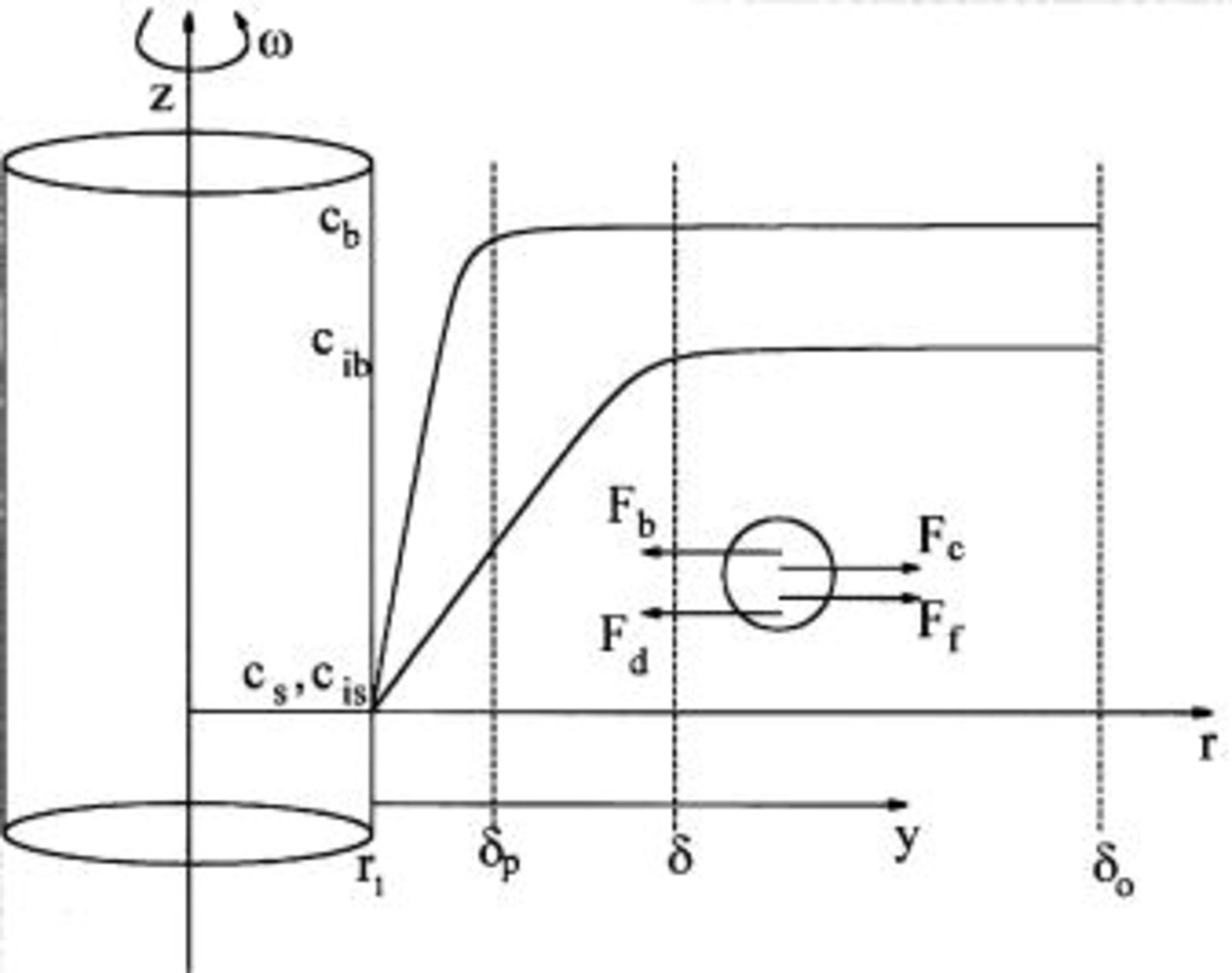
Figure 1. Schematic of the concentration profiles for the RCE and a force balance on a particle within the hydrodynamic boundary layer  . (In reality, the particle is much smaller than
 .)
Stojak and Talbot2 investigated the electrocodeposition of inert  particles in plated copper from an acidic copper sulfate solution of

 and
 of
 . In the electrolytic solution, the molecules of
 and
 dissociate predominately into three ionic species,
 ,
 , and
 ; only a very small fraction of the bisulfate ions dissociates, so that the concentration of
 is neglected.20–22 The concentration of
 is also negligible due to the low pH. Thus, the concentrations of these three species,
 ,
 , and
 , are considered. In this study, particle-particle interactions are not considered as the suspension of colloidal particles is dilute
 and inertial forces are negligible due to small particle size of
 . Electrokinetic effects were negligible as the zeta potential of the colloidal particles was zero in this highly conductive bath.
Mass transfer in an RCE system
Eisenberg et al.5, 6 extensively investigated mass transfer with an RCE and obtained the correlation of mass transfer rates in the form

where the Sherwood number  is a function of the Reynolds number
 , which is based on the diameter
 of the inner cylinder and the peripheral velocity
 of the inner cylinder, and the Schmidt number
 , which is a ratio of kinematic viscosity ν of the electrolyte to the diffusivity
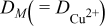
 of the reactive ion (i.e.,
 ). The convective mass transfer coefficient
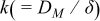 can be expressed as
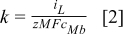
where  is the limiting current density,
 is the charge number,
 is the Faraday constant, and
 is the bulk concentration of the reactive ion. The diffusion layer thickness at an RCE using
 is calculated as

with units of the parameters as given in Table I.
Table I. List of values for physical properties.
| Physical property | Value at 
| Reference |
|---|---|---|

|

| 2 |
 of bulk solution |

| 2 |
 of bulk solution |

| 2 |
 of bulk solution |

| 2 |
|

| 29 |

|

| 29 |

|

| 29 |

|

| 2 |

|

| 30 |

| 1400 | |
| ν |

| 2 |

|
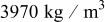
| 30 |

|
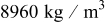
| 30 |
The surface concentration for the reactive ion  can be estimated from the fraction of the limiting current density23

where  is the current density at the cathode surface. Because the ratio of the hydrodynamic boundary layer thickness
 to the diffusion boundary layer thickness δ is proportional to
 by Eq. 1, we obtain24

In general, the value of  for an electrolytic solution is large, such that the thickness of the hydrodynamic boundary layer is much larger than that of the diffusion boundary layer; for
 in this study
 .25 Because the alumina particle size
 is small enough for Brownian diffusion to be important, the boundary layer thickness for particles
 was calculated from Eq. 3, with
 being substituted for
 , such that
 . Using the values in Table I, the three boundary layer thicknesses are compared in Table II for the RCE rotational rates of the experiments of Stojak and Talbot.2
Table II. Comparison of boundary layer thicknesses  for various RCE rotational rates.
| Rotational rate (rpm) | Particle  
| Ionic δ 
| Hydrodynamic  
|
|---|---|---|---|
| 500 | 7.5 | 36 | 476 |
| 1000 | 4.6 | 22 | 293 |
| 1500 | 3.5 | 17 | 221 |
Lagrangian description of a particle within the diffusion boundary layer
In order to determine the mass flux of particles  in an RCE system, the motion of a single nonconducting particle within the diffusion boundary layer thickness is assumed to be governed by Newton’s second law

where in cylindrical coordinates




and  is the mass of the single particle,
 is the density of the particle, and
 is the particle velocity. The diffusion force is
 , where
 is chemical potential,
 is Boltzmann’s constant,
 is temperature, and
 is concentration of the particles. The frictional force is
 , where
 is the resistance of a spherical particle to the fluid in Stokes flow. The centrifugal and buoyant forces are
 and
 , respectively, where
 is the mass of the displaced fluid, and
 is the density of the fluid. The gravitation force is not considered as it is perpendicular to the forces taken into account and also was found to be small for the
 diameter alumina particles considered (approximately 10 times smaller than the centrifugal force).26 In Searson’s studies,17, 18 the diffusional and gravitational forces were considered the main forces acting on a particle in a rotating disk electrode system. Also, as in those studies, stochastic (Brownian) motion of the particles is neglected.
If only the force balance in the radial direction  at steady state is considered, the inner product of Eq. 6 with the normal
 gives the following force balance

The particle flux  can then be calculated by substituting the radial velocity
 from Eq. 7 to obtain

where  is a parameter that represents the effect of the centrifugal force and
 is the diffusion coefficient of the particle. Note that the parameter
 depends on the density difference between the particle and fluid, particle size, the electrode rotational speed, and fluid viscosity. When the density of a particle is larger than that of the fluid, the buoyancy force is weaker than the centrifugal force, so that the force acting on a particle is always from the rotating cylinder.
By using the boundary layer thickness  , the mass flux for a particle at the surface in Eq. 8 may be approximated by

where  is the average mass transfer coefficient for a particle, as compared to the mass transfer coefficient for the reactive ion
 ,
 . By calculating the parameters
 and
 and the electrode surface concentration of reactive ions, the mass flux can be determined based on the flow characteristics. In the work of Shao et al. ,18 a similar relationship was developed for the particle flux, except that the two transport parameters represented the effects of the gravitational force and the diffusional flux for the RDE.
Instead of solving the convective-diffusion equation for a particle, a statistical approach is taken in which  is defined as the probability for particles to be in the neighborhood of an electrode. Then, the surface concentration of particle
 , where
 is estimated from experimental results. If
 , the surface concentration is zero, and as
 approaches 1, the surface concentration increases to the bulk concentration of particles. Thus, Eq. 9 can be written in terms of the bulk particle concentration as

Volume fraction of particles in the deposit
The volume fraction  of particles incorporated in a metal deposit can be expressed as a ratio of the incorporated volume of particles to the total volume of the composite17

where  is the number of moles of particles in the film,
 is the number of moles of metal atoms in the film,
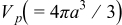 is the particle volume,
 is the particle radius,
 is the molar volume of the metal film, and
 is Avogadro’s number.
From the mathematical model for electrocodeposition of Celis et al. ,19 the flux of particles to the surface  is given by

where  is the flux of the metallic ions to the electrode, which is proportional to the current density from the reduction of metallic ions, where
 is the number of electrons transferred in the reduction reaction.
In electrocodeposition a maximum in the weight (or volume) percentage of particles incorporated as a function of current density has been observed frequently.1, 2 The parameter  was proposed by Celis et al.19 as the transition current density at this maximum incorporation from kinetic to mass transfer limited deposition. The variable α is equal to zero if
 for kinetic limited deposition and nonzero if
 for mass transfer control. Therefore, under kinetically controlled deposition, the ratio of the particle flux to metallic ion flux is directly equal to the respective molar concentration in the film
 . In this study, the values of
 and α are determined from fitting experimental data.
The ratio  can be expressed in terms of the volume fraction from Eq. 11
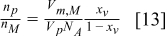
By combining Eq. 12, 13,  can be written as a function of volume fraction and current density that can be measured from experiments

By rearranging, the ratio of the total volume of particles  to that of the deposited metal
 can be determined

Finally, the volume ratio in Eq. 15 can be recast by substitution of  from Eq. 10 as

Vereeken et al.17 introduced a probability of particle incorporation to modify the surface concentration of the particle mass flux in Eq. 15, where the probability was assumed to be proportional to the deposition current. The surface concentration of particles was represented in terms of an extrapolated particle surface concentration and a characteristic current density at which the probability is 1. Based on the characteristic current density  , the volume ratio was divided into two regions depending on the magnitude of the current density being either larger or smaller than
 . The characteristic current density,
 , corresponds to the transition current density,
 , of the model of Celis et al.19 However, when
 , the volume ratio was taken as inversely proportional to the current density. In this study, using the definition from Celis et al. ’s model, we show that the volume ratio is proportional to current density to the power of α. When
 , the volume ratio equation reduces to the model of Vereeken et al.17 If
 , the volume ratio is independent of current density. To distinguish between the two regions with respect to
 ,
 and
 are used. When
 ,
 and the volume ratio will decrease as current density increases, whereas when
 ,
 and the volume ratio behaves according to Eq. 15. The magnitude of the volume ratio depends on the magnitude of the transport parameters,
 and
 , the probability
 , and the fitting parameters of
 and α. The dependence of volume ratio on current density in both regions is discussed later.
Calculation of ionic concentrations and potential
In a supporting electrolyte where no concentration gradients exist, the current density in the bulk solution is governed by Ohm’s law, and the current is carried by nonreactive ions, such as  and
 as in the acid copper plating system. As the electrical conductivity of the solution in a supporting electrolyte is very large, the potential gradient is very small. Within the diffusion boundary layer thickness, however, the electric field force competes with the concentration gradient in the movement of ions which carry the current.27 Although the concentration of the reactive ion is smaller than the nonreactive ions, the concentration gradient of the reactive ion is significant, as the current is due to the reduction of reactive species in a deposition process. To address the effects of an electric field and diffusion of a single reactive species in a supporting electrolyte solution, the transport equations for the ionic concentration and the electrostatic potential in a diffusion boundary layer δ in the absence of a particle were solved by the successive approximation as given in the Appendix
A perturbation method was used to obtain the asymptotic solutions for the ionic concentrations and the electrostatic potential gradient in the diffusion boundary layer28 for a  plating solution. The variables
 ,
 , and
 correspond to the concentration of
 ,
 , and
 , respectively. The solutions (including up to the second-order terms) of the normalized concentrations
 and potential
 within the ionic diffusion boundary thickness δ are




where  , and is used as the small parameter for the asymptotic solutions, which is reasonable for an acidic copper plating bath. Here,
 is the normalized current density divided by
 and ξ is the radial direction coordinate normalized by δ. The coefficients
 are given in the Appendix
 at the electrode is

where

and

In Eq. 21,  and
 are the contributions of the electric field and diffusion to the current density, respectively.
Results and Discussion
To understand the transport processes for an RCE, the contributions of the electric field and diffusion to the current density using the solutions of Eq. 21 were calculated for small values of  . As shown in Fig. 2, the errors from the asymptotic solution in Eq. 21 are 0.0525 for
 (thick line) and 0.0008 for
 (thin line). As ε is small (the solution is a well-supported electrolyte), the contribution of diffusion is dominant. In this study, the value
 for a plating bath of
 and
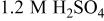 (Ref. 2) is used for all calculations. The diffusion of
 is the dominant process, which increases from
 to
 as the average current density increases. The current density due to electromigration of
 is negligible. Therefore, it is assumed that the current density is only due to diffusion; electromigration is ignored.
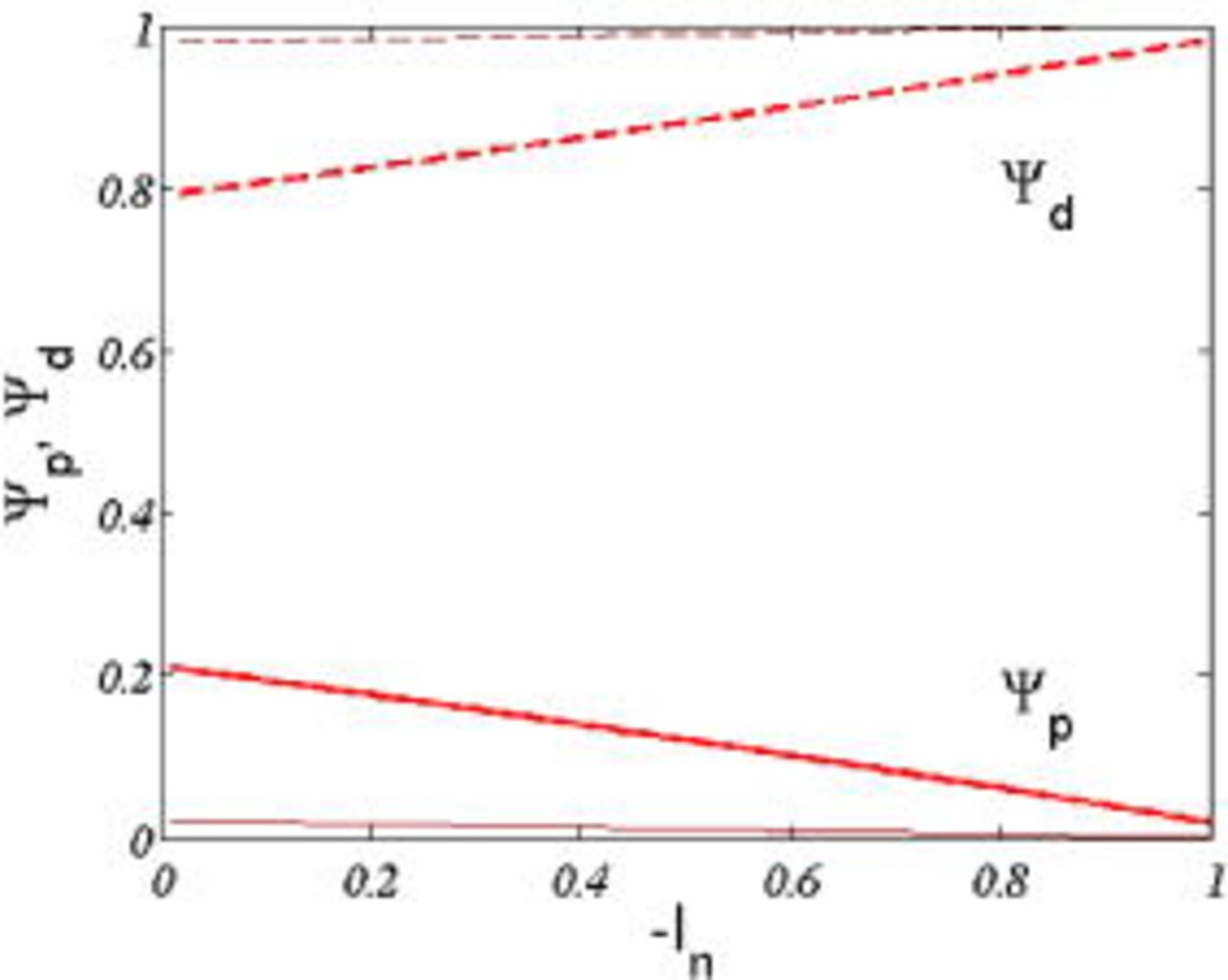
Figure 2. (Color online) The contributions of the electric field  and diffusion
 to carry the current as a function of
 , where the thin and thick lines correspond to
 and
 , respectively.
The concentration profiles of the three ionic species were calculated by Eq. 17, 18, 19 for a plating bath of  and
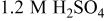 . The distribution of the concentration of each ion for
 is shown in Fig. 3, where each concentration is normalized by its bulk concentration. The concentration gradients for
 and
 counteract the gradient of the electrostatic potential, so that their fluxes are zero at the electrode surface, which induces the small change of concentrations of
 and
 in the diffusion layer.27 The potential gradient ∂Φ∕∂ξ as calculated from Eq. 20 is almost constant in the diffusion layer and is small in the bulk solution because of the high conductivity bath.
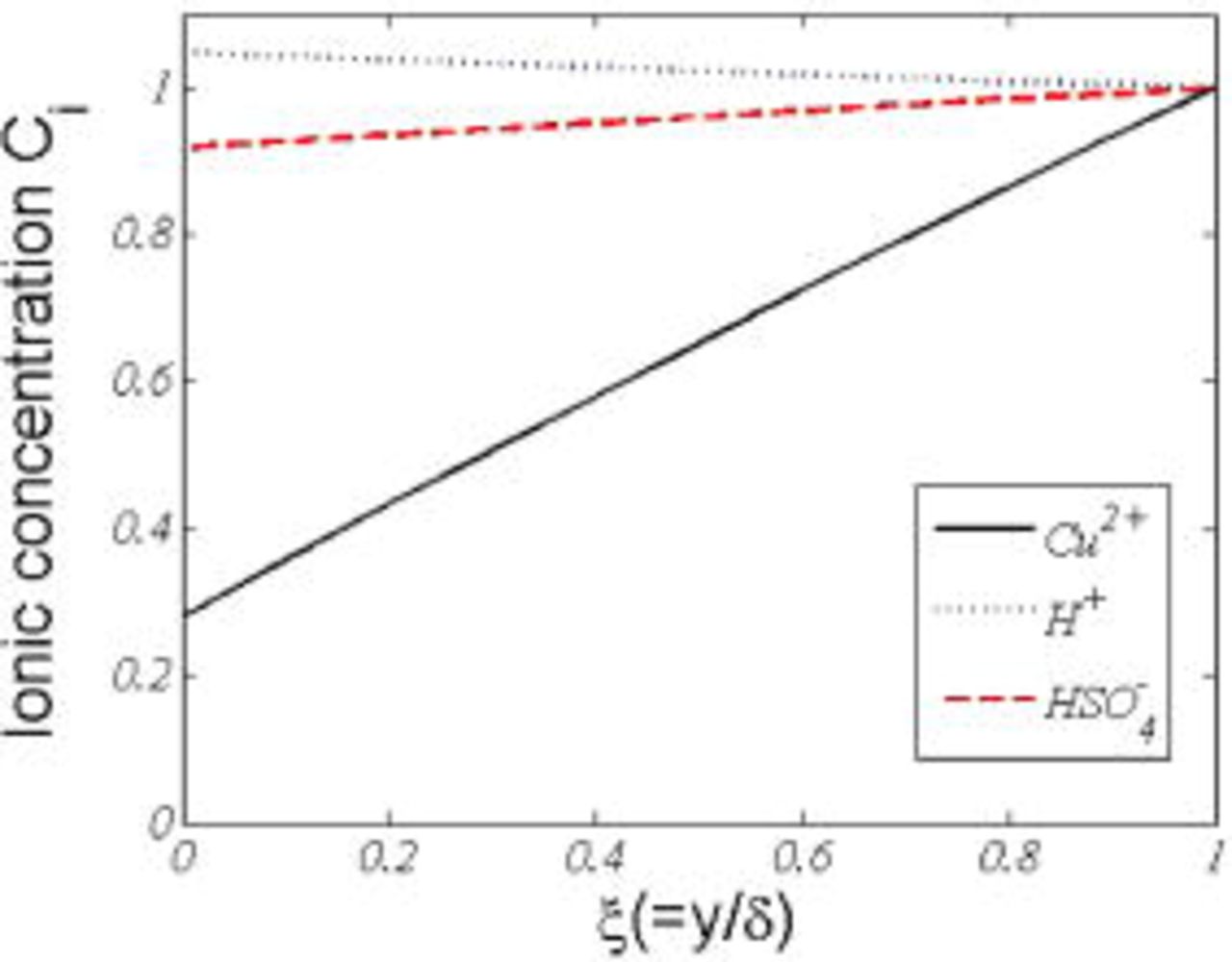
Figure 3. (Color online) Normalized ionic concentration profiles in the diffusion boundary layer, where  .
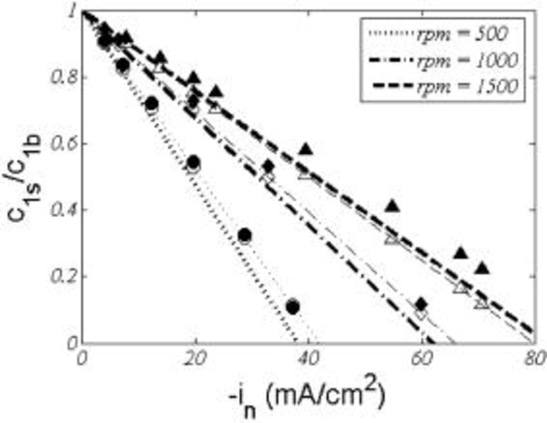
Figure 4 compares surface concentration for  as a function of current density calculated from experimental data of Stojak and Talbot2 for electrocodeposition with a particle loading of
 using Eq. 4 and predicted from the analytical solutions from Eq. 17. The surface concentration of
 is linear up to the limiting current density as determined from Eq. 4. The thin and thick lines for each set of data correspond to the surface concentration calculated from experimental limiting current density data2 and from
 using the diffusion layer thickness in Table I. At a low rotational speed of
 , the theoretical predictions agree well with experimental results. At the higher rotational rate, the values from the asymptotic approximation are somewhat higher than the experimental results. This difference may be due to the absence of particles and convection in determining the surface concentration from the analytical solution of Eq. 17.



Before discussing the results of the particle incorporation model for the RCE of Eq. 16, the two transport parameters  and
 as defined in Eq. 9, which represent the effect of the centrifugal force and the mass transport of the particle, respectively, are discussed. Figure 5 illustrates the magnitude of
 and
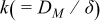
 as a function of particle radius. For comparison, the lines at the top-right corner in Fig. 6 denote the mass transfer coefficient,
 , for
 . The difference between
 and
 is due to the difference between the two diffusion boundary layer thicknesses and diffusivities for the reactive ion
 and a particle
 , as shown in Table I and II. Thus, the effect of mass transfer for the reactive species is larger than that for the particle. The reason is that a reactive ion has a higher diffusivity than a particle, even if
 is less than δ. The ratio
 is then always larger than unity and approaches a constant value as the particle radius increases. Increasing the speed of the rotating cylinder has a larger effect on
 than on
 , because
 is proportional to
 , while
 is proportional to
 by Eq. 5. Below a particle radius of
 depending on the RCE rotational rate, the effect of mass transfer is more dominant. Above this particle radius, the centrifugal force is more pronounced as
 and
 are proportional to
 and
 , respectively. Therefore, it is expected that a thin boundary layer and a small particle size would result in an increased particle incorporation in the deposit.
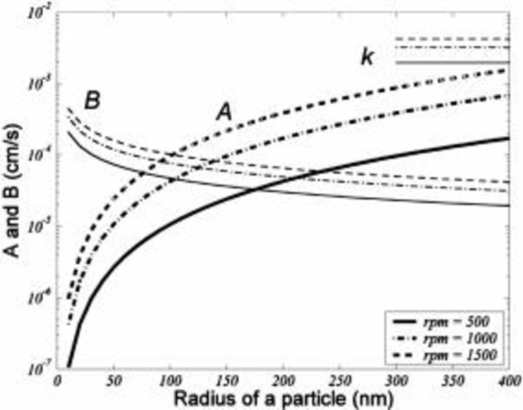
Figure 5. Comparison of model parameters  and
 as a function of particle radius for various rotational speeds with
 ,
 ,
 ,
 , and
 . The thick and thin lines correspond to
 and
 , respectively. The lines at the top-right corner show the mass transfer coefficient
 for
 .
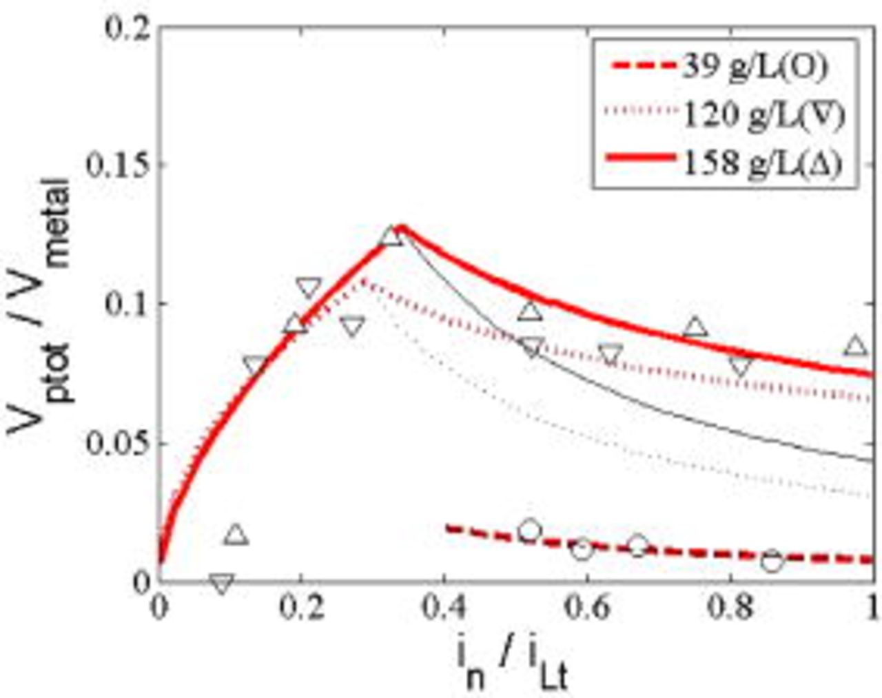
Figure 6. (Color online) The ratio of particle volume  to metal volume
 in the composites at the rotating speed of
 . The dashed, dotted, and solid lines correspond to a particle loading of
 ,
 , and
 , respectively, whereas the symbols are experimental data.
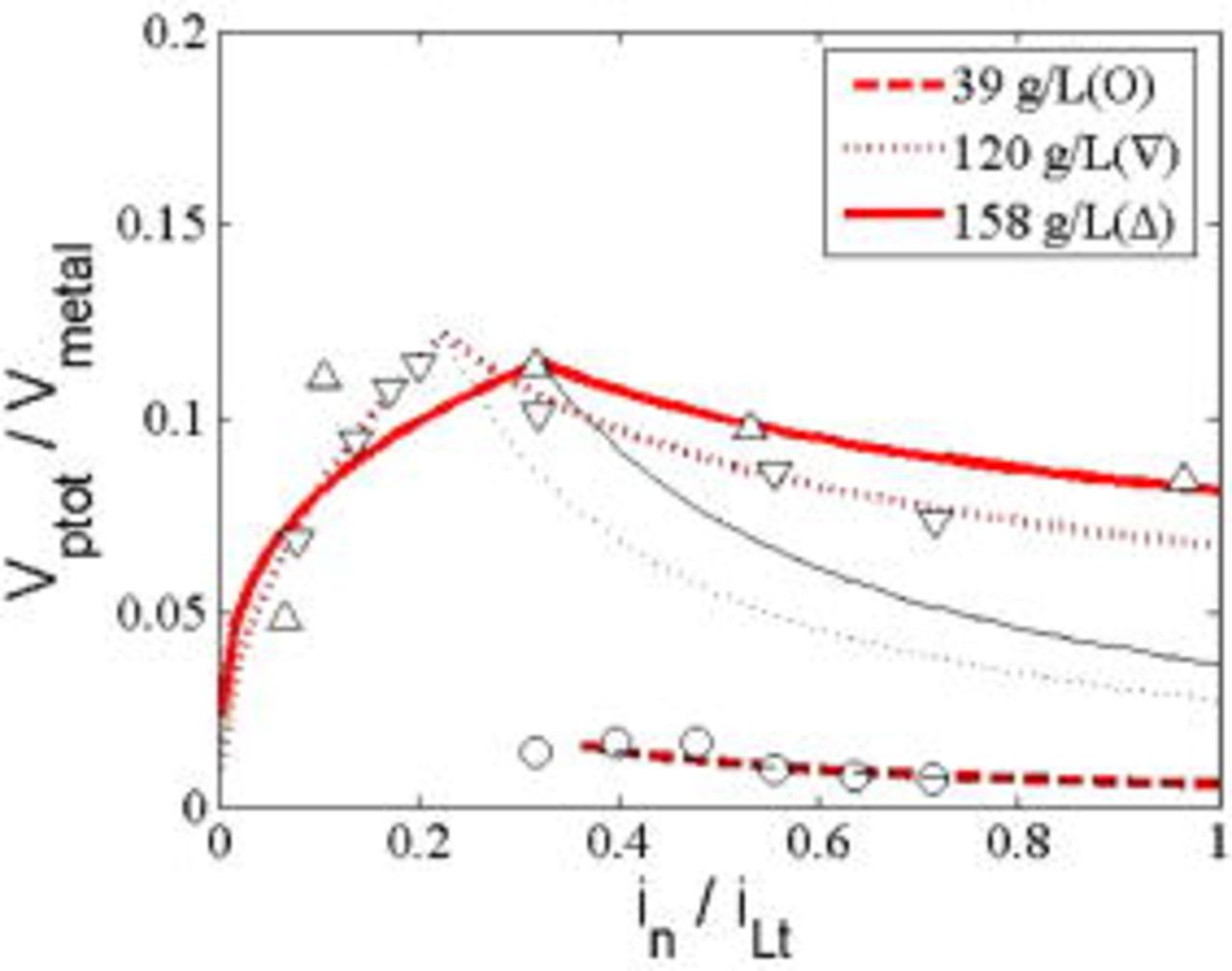
Figure 7. (Color online) The ratio of particle volume  to metal volume
 in the composites at the rotating speed of
 . The dashed, dotted, and solid lines correspond to a particle loading of
 ,
 , and
 , respectively, whereas the symbols are experimental data.
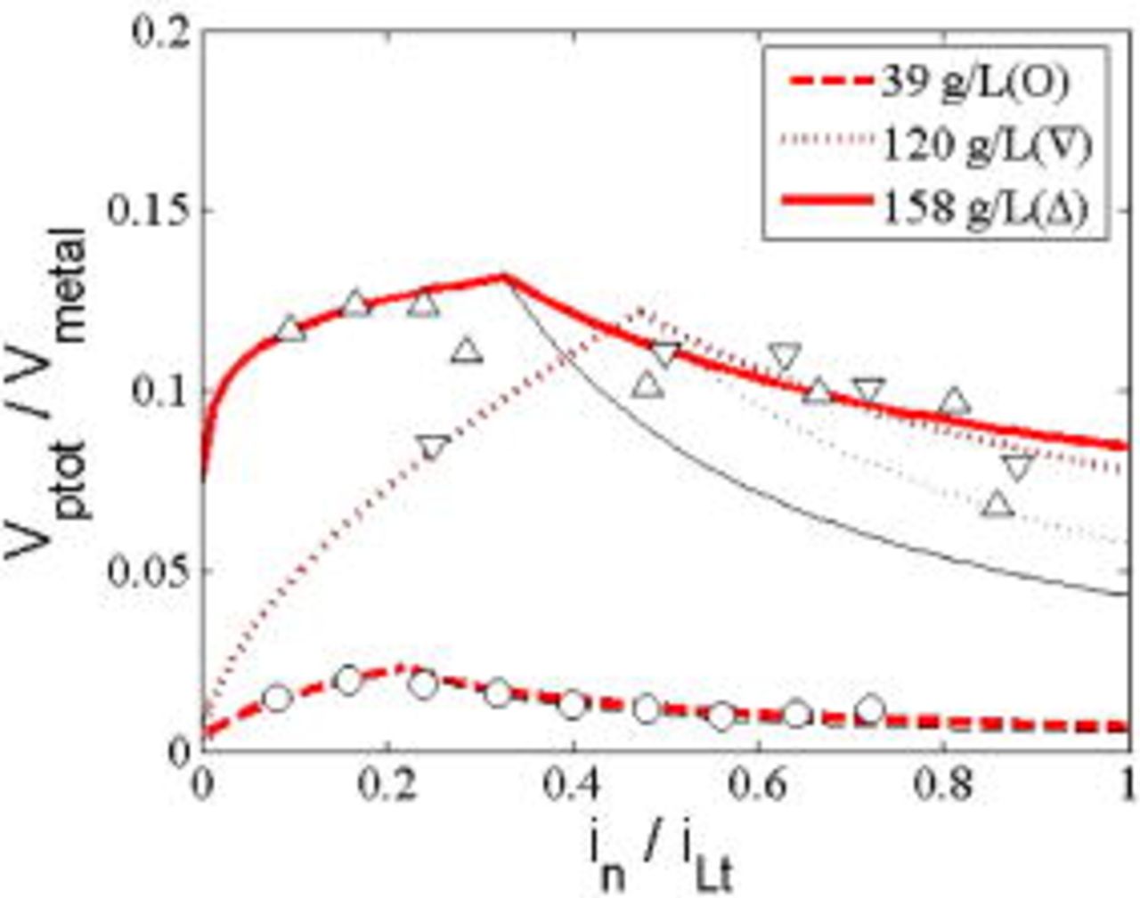
Figure 8. (Color online) The ratio of particle volume  to metal volume
 in the composites at the rotating speed of
 . The dashed, dotted, and solid lines corresponds for a particle loading of
 ,
 , and
 , respectively, whereas the symbols are experimental data.
In order to approximate the surface concentration of particles, Eq. 9 can be rewritten as follows
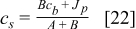
where the order of magnitude of the particle mass flux  is
 as calculated from Eq. 14 using experimental results,2 which is much less than
 , which is
 . This is due to the very thin diffusion boundary layer thickness and the low particle mass flux. However, for our case of
 ,
 and the probability
 is equal to
 . The estimated probabilities
 at each rotational speed shown in Table III are independent of particle loading, and these results were used to predict the volume ratio in Eq. 14. The probability
 is thus dependent upon the transport parameters of the system,
 and
 . With
 , i.e., the particle radius is very small as shown in Table IV and Fig. 5, the surface concentration is very close to the bulk concentration, i.e.,
 . Thus, nearly all of the particles at the surface become incorporated into the deposit.
Table III. The probability  and the theoretical limiting current density for a rotational speed for a particle diameter of
 .
| Rotational rate (rpm) |

|
 
|
 
|
 
|
|---|---|---|---|---|
| 500 | 0.9942 | 0.67 | 1.16 | 38 |
| 1000 | 0.9858 | 2.71 | 1.88 | 62 |
| 1500 | 0.9762 | 6.10 | 2.50 | 82 |
Table IV. The fitting parameters for the RCE electrocodeposition model.
| Particle loading (g/L) | Rotational speed (rpm) |

|

|

|
|---|---|---|---|---|
| 39 | 500 | 0 | N/A | 0.39 |
| 1000 | 0 | N/A | 0.35 | |
| 1500 | 0.2 | 1.5 | 0.22 | |
| 120 | 500 | 0.6 | 1.5 | 0.29 |
| 1000 | 0.6 | 1.5 | 0.23 | |
| 1500 | 0.4 | 1.6 | 0.47 | |
| 158 | 500 | 0.5 | 1.6 | 0.34 |
| 1000 | 0.7 | 1.3 | 0.32 | |
| 1500 | 0.6 | 1.1 | 0.33 | |
| Average value |

|

|

|
Stojak and Talbot2 investigated extensively electrocodeposition using an RCE system, where the deposition conditions ranged from kinetically limited to mass transfer limited regions. Their experimental data were compared with the theoretical prediction from Eq. 16 of the ratio of particle volume to metal volume in the film, 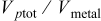 . The best fit of the model to the experimental data was made by adjusting the parameters α and
 . As discussed, the value for α was chosen to be less than unity when
 ; the volume ratio decreases as the current density increases in the mass transfer limited region. Celis et al.19 plotted the weight percentage of incorporated particles versus average current density, where
 was the maximum value which represents the transition from the kinetic limited region to the mass transfer limited region. In this study,
 was chosen to adjust the magnitude of the volume ratio.
The experimental data of Stojak and Talbot2 were measured at three electrode rotational rates (500, 1000, and  ) and three particle loadings (39, 120, and
 ). The volume ratio vs the current density normalized by the limiting current density,
 (as listed in Table III) for these nine sets of data is compared with the model results in Fig. 6, 7 and 8 for each rotational rate. The fitting parameters are summarized in Table IV. As no data were available at small current densities at a particle loading of
 at 500 and
 ,
 could not be determined.
As shown in Fig. 6, 7 and 8, the model agrees well with the experimental results for data both below and above the transition current density. For 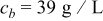 and a low level of particle incorporation (a volume ratio less than 0.02), the
 equals 0 at low rotational rates and 0.2 at
 . As the particle loading increased to
 and
 , the model prediction with
 shows a large deviation from experimental results. Although the value of
 appears to slightly increase with particle loading (with an average value of 0.5), the values of
 and
 are nearly constant for all the data sets with average values of 1.4 and 0.33, respectively.
The difference between our results and those of the Celis model19 is that the curve for  is not a straight line;
 is not equal to 2. The main concept of the Celis model is the competition of diffusion rate between particles and ions across the diffusion layer; the parameter α compensates for the relative diffusion speed of the particles. It was assumed that in the kinetically controlled region the diffusion speed for particles and ions was the same, so that the relationship was linear
 . However, the experimental data from Stojak and Talbot show that the rate of particle incorporation is larger than that of deposited ions under kinetic control, i.e.,
 . In the mass transfer controlled region the reactive ion deposition rate is faster than that of particles, and the diffusion of particles becomes the controlling step. At a higher current density, this distinction is more obvious. This results in a positive value of
 .
Conclusions
A model for electrocodeposition on an RCE was developed to predict the particle incorporation volume ratio which agrees well with experimental data. The asymptotic solution for the concentration profiles for ions within the diffusion boundary layer showed that diffusion of the reactive species in a supporting electrolyte solution is the dominant process to carry the current at the cathodic surface; the contribution of electromigration is negligible. The ratio of the total volume of particles to that of the deposited metal was expressed as a function of two transport parameters, current density, a probability  , and two experimental fitting parameters (
 and α). The model can be used easily to predict the volume ratio in the kinetically and mass transfer limited region of electrocodeposition with only few experimental data points.
University of California, San Diego, assisted in meeting the publication costs of this article.
List of Symbols

| transport parameter for centrifugal force |

| particle radius, m |

| concentration of  , 
|

| concentration of  , 
|

| average mass transfer coefficient for particles |

| concentration of particles, 
|

| concentration of  species, 
|

| normalized concentration of  species by 
|

| particle diameter, m |

| diameter of the inner cylinder, m |

| minimum distance between a particle and an electrode, m |

| diffusivity, 
|

| Faraday’s constant,  . |

| gravitation acceleration rate, 
|

| current density, 
|

| normalized current density by 
|

| limiting current density, 
|

| transition current density, 
|

| mass flux of particles on an electrode surface, 
|

| mass flux of deposited atoms on an electrode surface, 
|

| mass transfer coefficient  , m/s |

| Boltzmann’s constant |

| single particle mass, kg |

| mass of the displaced fluid  , kg |

| unit normal vector pointing out an electrolyte solution |

| number of moles of particles in a deposited film |

| number of moles of metal atoms in a deposited film |

| Avogadro’s number |

| probability of particle being at the surface |

| gas constant, 
|

| coordinate perpendicular to an electrode surface |

| inner cylinder radius, m |

| Reynolds number |

| Schmidt number |

| Sherwood number |

| temperature, K |

| velocity vector of a fluid, m/s |

| peripheral velocity at  , m/s |

| fluid velocity at the center of a particle, m/s |

| molar volume of a deposited film |

| volume of a particle, 
|

| mobility of  species defined by 
|

| coordinate defined as 
|

| charge number |
Greek letters
| α | model fitting parameter |

| model fitting parameter when 
|

| model fitting parameter when 
|
| β | friction coefficient 
|
| δ | ionic boundary layer thickness, m |

| viscous sublayer boundary layer thickness, m |

| boundary layer thickness for particles, m |
| ε |

|

| density of the cathodic deposit, 
|

| density of a particle, 
|

| density of the electrolyte solution, 
|
| μ | viscosity of the electrolyte, 
|
| ν | kinematic viscosity of the electrolyte, 
|
| ω | electrode rotational rate, rad/s |
| ϕ | electrical potential, 
|
| Φ | normalized electrical potential by 
|
| ξ | normalized coordinate 
|

| volume fraction of inert particles incorporated in a composite film |
Subscripts

| bulk solution |

| deposited species |

| particle |

| electrode surface |
: Appendix
The Nernst-Planck equation for the molar flux of the  th species is

where  is the mobility,
 is the charge number,
 is Faraday’s constant,
 is concentration,
 is diffusivity,
 is the gas constant,
 is the absolute temperature,
 is the velocity field of the fluid, and ϕ is the electrostatic potential function.29 The first, second, and third terms on the right-hand side of Eq. 1 are the contributions of the flux due to migration in an electric field, the diffusion due to a concentration gradient, and convection from the velocity of the fluid, respectively. For convenience, the subscripts
 correspond to
 ,
 , and
 , respectively. For an acidic copper sulfate plating bath,
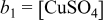 and
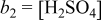 , such that
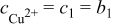 ,
 , and
 in the bulk region, where
 is much larger than
 . An electrolytic solution is governed by the electroneutrality condition

except in the thin regions near charged boundaries. The mass balance for each species with no reaction requires

where the fluid is incompressible. Because the boundary layer thickness δ is usually much smaller than the inner cylinder radius  , the distribution of ionic concentrations only in the direction of
 in rectangular coordinates is considered. When it is assumed that the fluid flows perpendicular to the
 plane, the convection term on the left-hand side of Eq. 3 vanishes for the two-dimensional analysis.
The following dimensionless variables are introduced to simplify the governing equation Eq. 3

The governing equations at steady state can be written as

The boundary conditions on the surface of an electrode  are

and at the diffusion boundary layer 

where ε is a small parameter defined by  and is assumed to be much less than 1
 . We approximate the solutions of
 and Φ in a series expansion as

where the subscripts  denote the
 th order of magnitude. Note that
 for the expansion of
 . By substituting these relations into Eq. A-5 through A-7, we obtain


The equations of order of magnitude of  from Eq. 5 are

The boundary conditions at  are

and at the boundary layer 

The solutions for  can be easily obtained by

The first-order equations to  from Eq. 5 are

The boundary conditions at  are

where the flux of  species is balanced by the applied current density and the fluxes of
 and
 are zero due to a no-penetration condition. Because
 is zero,
 is linear from Eq. 15. At the boundary layer
 , the concentrations are those of the bulk

The solution for  is obtained using the boundary conditions of Eq. 16 and Eq. 17. The equation for the electrostatic potential
 is derived by summing Eq. 15 for all species and using the electroneutrality condition, i.e.,
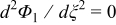 . One integration gives
 , where
 is an arbitrary constant and is determined from the electroneutrality condition. The solutions for
 and
 are obtained from Eq. 11 using the boundary conditions of Eq. 16, 17. The first-order solutions by simple algebra are



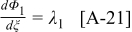
Because  from Eq. 15,
 .
At  ,
 . Substituting
 and arranging the resultant equation, the arbitrary constant
 is then given by
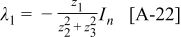
In a similar way, the second-order equations to  are determined from Eq. 5

The boundary conditions at  are

and at 

The procedure to obtain the solutions is the same as that of the first-order case. The second-order solutions are




where



Therefore, the solutions up to the second order of magnitude are




Therefore, the solutions of  and
 can be rewritten by the dimensionless variables defined by Eq. 4.
