


Abstract
A global 2 °C climate target is projected to generate significant economic benefits. However, the presence of fossil fuel assets that are stranded as a consequence of climate change mitigation could complicate cost-benefit considerations at the country level. Here, we quantify the spatial distribution of stranded asset costs (SAC) together with that of the GDP benefits of climate mitigation (BCM). Under a 2 °C scenario, global total SAC is $19 trillion while global BCM is $63 trillion by 2050. At the country level, the sign of a country's net benefit, the difference between BCM and SAC, is largely determined by the sign of its BCM. Net benefits are broadly positive across subtropical and tropical countries where high baseline temperatures imply GDP damage from climate change and negative across temperate countries where low baseline temperatures imply GDP gains. Notably, even major fossil fuel producers such as India, China, USA, and Saudi Arabia are projected to receive positive net benefits from a 2 °C scenario by 2050. Overall, 95% of global net benefit will be borne by low and lower-middle income countries. These results could inform the geopolitics of global climate change cooperation in the decades to come.
Export citation and abstract BibTeX RIS

Original content from this work may be used under the terms of the Creative Commons Attribution 4.0 licence. Any further distribution of this work must maintain attribution to the author(s) and the title of the work, journal citation and DOI.
1. Introduction
Climate change mitigation will yield substantial global benefits. Avoided losses in global gross domestic product (GDP), a component of total potential benefits, are estimated to range from $100 to $400 trillion by 2100 under the 2 °C global climate target compared to a business-as-usual scenario before the Paris Agreement [1, 2]. At the same time, the dramatic decarbonization required to achieve such a target will incur a variety of costs [3], prompting trade-offs across other economic and social priorities. One class of cost for many countries is the lost value of their fossil fuel assets [4, 5], estimated to be $4 trillion between 2016–2035 [6] and $12 trillion between 2011–2100 [7]. These 'stranded asset' costs (SAC) have received increasing attention, as exemplified in the political opposition against language to 'phase down' fossil fuels during the Glasgow meetings under the United Nations Framework Convention on Climate Change [8, 9].
SACs are unevenly distributed across countries, and depend on a country's endowment of fossil fuel reserves and extraction costs [10–12]. The GDP benefits of climate mitigation (BCM) may also be highly heterogeneous in part because the nonlinear GDP-temperature relationship implies economic losses in hotter locations while colder locations experience economic gains [13, 14]. This prompts a series of questions. Are the same countries with high SAC also those with high BCM? For which countries do BCM exceed SAC? How do these spatial patterns change over time horizons as country-level SAC and BCM evolve dynamically? Such dynamics are of interest as fossil fuel reserves deplete over time and marginal GDP losses grow for hotter locations as temperatures increase. We address these questions by conducting a joint analysis of country-level SAC and BCM. While SAC and BCM are incomplete measures of total climate policy costs and benefits, which itself may not fully explain climate policy adoption, our analysis may nonetheless shed light on existing barriers to international climate policy cooperation and how they could evolve in the decades to come.
This study quantifies SACs associated with the value of fossil fuels that a country forgoes from reduced fossil fuel production under a global 2 °C target [15]. Following van der Ploeg et al [16], we define SAC as the foregone discounted net present profits from fossil fuel production for a country under a 2 °C target relative to a pre-Paris Agreement business-as-usual (BAU) scenario between 2020–2050. Country-level BCM is the country-level avoided GDP loss of a 2 °C global target, based on an econometrically estimated GDP-temperature damage function [17]. We combine these two measures, showing how the net benefits from these two measures are distributed across countries and according to countries' income groups. To examine how net benefits evolve over time, we present net present values for both 2020–2030 and 2020–2050 time horizons as well as show payback periods.
2. Methods and materials
Temperature projections follow Representative Concentration Pathways (RCPs), and GDP and population trajectories come from the Shared Socioeconomic pathways (SSPs) [18]. RCP6.0 is used as our 'business-as-usual' or pre-Paris Agreement scenario (i.e., BAU scenario) [19, 20], while RCP 2.6 is used as the scenario (i.e., 2 °C scenario) whereby global mean temperature increase is capped below 2 °C (table S1). Socioeconomic assumptions follow SSP2.
The total cost of climate change mitigation is composed of (a) the change in profits for producers and (b) the change in welfare for consumers due to climate policy. Producers include both firms in sectors that use fossil fuels and those in sectors that use non-fossil (e.g., renewable) fuels. In this paper, we focus on the forgone profits of fossil fuel producers, calculated as the forgone net present profits from fossil fuel production under a global 2 °C relative to business-as-usual. As such, we consider an incomplete measure of the total cost of climate policy while omitting profit changes to non-fossil fuel production and welfare changes in consumers, both of which may play a role in determining support for climate policy. As is standard in non-renewable resource settings, a country's stranded asset profit is the sum of resource rents across its fossil fuel deposits. A deposit's resource rents, in turn, are determined by its resource grade and scarcity [21, 22]. The stranded asset costs are only those associated with forgone profits for fossil fuel extraction and not any resulting local environmental changes due to lowered fossil fuel extraction.
Our analysis of fossil fuel profits is at the country level. This implicitly assumes countries own property rights to their fossil fuel resources, which indeed is the case for 90% of global fossil fuel reserves [23]. Furthermore, we assume either (a) countries are also fossil fuel extractors or (b) the global market to extract fossil fuel resources is perfectly competitive, as a country receives all profits in either case. In particular, under perfect competition, profits are zero for the fossil fuel extractor, such that revenue less extraction cost for an extracting firm equals the royalty lease paid to the country. Failure of either assumption would not affect our estimate of forgone profits but rather how that profit is split between countries that own the fossil fuel reserve and the fossil fuel extractor. In that case, one could view our forgone profit estimate as that associated with fossil fuel reserves owned by a particular country rather than that actually received by the country.
Forgone profits are calculated using projected fossil fuel prices and production generated by Integrated Assessment Models (IAMs) in the ADVANCE database under SSP2 [24, 25]. We obtain projected country-level fossil fuel price and production for each scenario and IAM (i.e., AIM/CGE, IMAGE, POLES, WITCH) from the IPCC AR6 library [26] in the ADVANCE database (table S2). We use ADVANCE's 'Reference' and '2020 WB2C' scenarios as our BAU and 2 °C scenarios, respectively. All projected price and production data are normalized to observed 2018 values from the World Bank [27] and the U.S. Energy Information Agency [28], respectively, to ensure continuous time series trajectories. Data on fossil fuel reserves come from the Federal Institute for Geosciences and Natural Resources (BGR) [29]. Data on reserve-level extraction costs for oil and natural gas come from the Rystad database [30, 31], and for coal from Welsby et al [11]. We perform analyses for the following 12 countries/regions: Brazil, China, India, Japan, Russia, USA, European Union, Latin America, Middle East and Africa, rest-of-Asia, rest-of-OECD, rest-of-Reforming Economies. For multi-country regions, we assume that countries in that region follow the same fossil fuel price and production path. We classify countries into high, upper-middle, lower-middle and low income groups, following definitions provided by the World Bank [32].
The benefits of climate change mitigation are measured in terms of avoided GDP losses using a historically-estimated econometric relationship between GDP and temperature from Burke et al [17]. This too is an incomplete measure of climate policy benefits, notably missing non-market benefits such as health impacts. The code and data used in our study are compiled from Ricke et al [33]. In the main text, we use a 3% discount rate to calculate values, presented in 2018 dollars. Our main focus is the 2020–2050 time horizon, though we also present net present values for the 2020–2030 horizon.
2.1. Calculating SAC
The global carbon budget is estimated to be 980−1420 gigatons (Gt) of CO2 if the global economy is to limit the global mean temperature increase to below 2 °C at a two-thirds probability [34]. By contrast, global total economic reserves of fossil energy resources would emit 2900−3500 Gt of CO2e if combusted [10, 35]. Thus, in the absence of large-scale carbon capture and storage, a substantial share of global fossil fuel reserves must remain underground [10, 25]. We translate this reduced global demand for fossil fuel onto country-level fossil fuel production using established mitigation scenarios from IAMs. To calculate country-level foregone profit, or SAC, we construct country-level fossil fuel supply curves using deposit-level extraction cost data, and determine the change in country-level profits between BAU (or pre-Paris Agreement) and 2 °C scenarios due to loss in production from marginal deposits according to extraction cost.
Specifically, for each country/region i, fossil fuel k, year t, and scenario s ∈{BAU, 2 C}, each IAM model generates endogenous fossil fuel price, ps ikt, and total production, qs ikt. Each country has deposit d for fossil fuel k with heterogeneous reserves, rikdt, and constant extraction costs, cikdt. Deposits enter production in the order from low to high extraction cost until total production, qs ikt, is met. Denote the set of deposits in production for country i, fuel k, in year t as Ds ikt. We define the deposit-weighted country-level extraction cost as
The discounted profit between 2020–2050 from extracting fuel k for country i is
where δ = 0.03 is the discount rate. Finally, we define SAC for country i as the difference in discounted profit, summed across fuels, between the BAU and 2 °C scenarios
In a few countries, the domestic fossil fuel production may increase slightly to offset increased global fossil fuel price increases as large fossil fuel producers decrease production. For these countries, the SAC may be negative, which occurs for 3 out of the 169 countries analyzed. Our benchmark country-level SAC is the median value across AIM/CGE, IMAGE, POLES, and WITCH IAMs. We also present SAC values for each IAM.
2.2. Calculating BCM
Following Burke et al [17] the functional relationship between country i's growth rate in Gross Domestic Product (GDP) per capita and its average surface temperature in year t is
where the parameters  and
and  are econometrically estimated using historical data by Burke et al, 2015 [26] and
  is projected population-weighted country-year temperature under scenario s, also obtained from Burke et al [1]. Next, define Δit as the additional effect of warming on GDP per capita growth in country i and year t compared to that country's average historical temperature,
Let  be the baseline growth rate of GDP per capita and
  be the population under SSP2, obtained from the International Institute for Applied System Analysis [36]. GDP under climate change is then


As with SAC, BCM is defined as the discounted net present GDP between the two scenarios
2.3. Robustness
Our main results are calculated over the 2020–2050 horizon. We also present results for the 2020–2030 horizon to examine how impacts over a longer horizon affect SAC and BCM values. We further conduct several robustness checks. First, calculate SAC by including the value of stranded fossil fuel infrastructure. Second, we replace our baseline 3% discount rate with a 5% discount rate. Third, we present SAC values under separate IAM projections. Fourth, we calculate BCM under alternative SSP scenarios. Fifth, we calculate the net benefits on a per capita basis. These results can also be found via our online tool https://climate-change.shinyapps.io/generation_gap/.
3. Results
For the 2020–2030 time horizon, the median value of total global SAC under a 2 °C target across IAMs is $3.8 trillion (in 2018 dollars), with a range of $2.3 trillion (AIM/CGE) to $13 trillion (WITCH) (figure 1(a)). This is on par in magnitude with the global BCM under SSP2 with a value of $4.8 trillion (figure 1(c)). There is little variation in global BCM across SSP scenarios due to the limited temperature variation across the scenarios by 2030 (figure 1(c)).
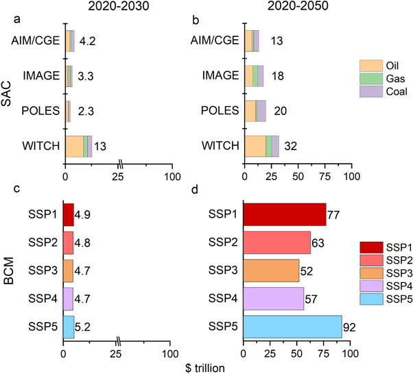
Figure 1. Global Stranded Asset Costs (SAC) and Benefits from Carbon Mitigation (BCM). (a) Global SAC across Integrated Assessment Models (IAMs) by fossil fuel for the 2020–2030 horizon. (b) Same as (a) for the 2020–2050 horizon. (c) Global GDP-based BCM across Shared Socioeconomic Pathways (SSP) for the 2020–2030 horizon. (d) Same as (c) for the 2020–2050 horizon.
Download figure:
Standard image High-resolution imageThe difference between global total BCM and SAC becomes more pronounced over the 2020–2050 horizon as marginal GDP damages increase with higher temperatures because of the nonlinear GDP-temperature damage function. Between 2020–2050, the median total SAC across IAMs is $19 trillion (in 2018 dollars), with a range of $13 trillion (AIM/CGE model) to $32 trillion (WITCH model) (figure 1(b)). By contrast, the global BCM under SSP2 is over three times larger at $63 trillion (figure 1(d)). There is now also greater variation in global BCM across SSP scenarios with a range of $52 trillion (SSP3) to $92 trillion (SSP5) (figure 1(d)).
Half of the 2020–2050 median global SAC comes from stranded oil reserves ($9 trillion), followed by stranded coal reserves ($6 trillion) and then stranded natural gas reserves ($4 trillion). When adding the cost of stranded fossil fuel infrastructure, the median 2020–2050 global SAC increase to $22 trillion (figures S1–S2). When we replace our benchmark 3% discount rate with a 5% discount rate, the range of global SAC across IAMs is $10–24 trillion (figures S3–S4). By comparison, Bauer et al23.estimate a global SAC of $12 trillion using the REMIND model and a 5% discount rate.
SACs are highly heterogeneous across countries and regions. Regionally, North America, Asia and Eastern Europe experience the largest SACs, while Western European, Latin American and Sub-Saharan African countries generally incur lower values (figures 2(a) and (b)). At the country level, Russia incurs the largest SAC ($2.6 trillion), closely followed by China ($2.6 trillion) and Saudi Arabia ($2.4 trillion) over 2020–2050. Iran incurs over $1 trillion in SAC while USA, Iraq, India, Canada, Qatar and Australia will experience over $0.5 trillion of SAC (table S3) over 2020–2050.

Figure 2. Distribution of SACs and BCMs across countries. (a) Country-level median SAC across IAM models for the 2020–2030 horizon. (c) Country-level BCM under SSP2 for the 2020–2030 horizon. (e) Country-level BCM (b) minus SAC (a) for the 2020–2030 horizon. (b), (d), (f). Same as panels (a), (c), (e) for the 2020–2050 horizon.
Download figure:
Standard image High-resolution imageLikewise, there is considerable heterogeneity in BCM across countries and years. Tropical and subtropical countries generally benefit from climate change mitigation. By contrast, some temperate countries incur smaller or even negative BCM because the quadratic GDP-temperature damage function exhibits a global optimum with temperate countries located on the cooler side of the optimum. This dispersion widens as the time horizon lengthens from 2020–2030 to 2020–2050 as marginal temperature-induced GDP losses become larger (figures 2(c) and (d)). Between 2020–2050, India is expected to receive the highest BCM at $24 trillion, while Russia incurs the lowest BCM at -$6 trillion (table S4).
Turning to net benefits, as measured by BCM minus SAC, countries typically fall in three categories, broadly defined by whether BCM or SAC determines the sign of a country's net benefit and why. The first category are countries with large positive BCMs and small SACs and thus positive net benefits. These countries tend to be in subtropical and tropical regions where baseline high temperatures imply large avoided GDP losses from climate policy but have few fossil fuel reserves. Between 2020–2030, net benefits of climate change mitigation are positive in many countries across Latin America, Africa, South Asia and Southeastern Asia (figure 2(e)). Net benefits become positive across almost all countries in these regions by 2050 (figure 2(f)).
The second category are countries with large negative BCMs which reinforces positive SAC values, resulting in negative net benefits. For these countries, primarily consisting of Europe, Canada, and Russia, net benefits are negative across both 2020–2030 and 2020–2050 horizons, largely because higher temperatures can increase economic activity in these colder locations [13, 17]. SAC values exacerbate the economic burden of climate change mitigation for these countries. Between 2020–2050, net benefits are -$9 trillion for Russia and -$3 trillion for Canada (figure 2(f)).
The last category consists of countries with large SACs but of which an even larger BCM still determines the sign of net benefits. These countries include India, China, USA, and Saudi Arabia, which are projected to experience net benefits of $23, $6, $2, and $0.4 trillion by 2050, respectively. A common feature unifies the countries across these three groups: the sign of their net benefit by 2050 is primarily determined by their BCM, not their SAC. There are three notable exceptions to this: Australia, Iran, and Iraq all experience negative net benefits because sizable fossil reserves imply a higher SAC and BCM.
We next consider total SAC, BCM, and BCM minus SAC by income group. In general, higher income countries experience larger SACs while lower income countries experience higher BCMs. Specifically, high and upper-middle income countries are projected to experience 88% and 89% of the global SAC by 2030 and 2050, respectively (figures 3(a) and (b)). It is notable that, except for India ($0.9 trillion), the countries that bear the top ten highest SACs over 2020–2050 are all high- and upper-middle-income countries (Table S3). The total SAC share borne by low income countries is under 1% for both 2030 and 2050 time horizons. By contrast, for BCM, about two-thirds of the global BCM is borne by low and lower-middle income countries by both 2030 and 2050 (figures 3(c) and (e)). Combining SAC and BCM values, by 2050, 95% of global net benefits of a 2 °C global target are projected to be experienced by low and lower-middle income countries, with largest values for lower-middle income countries at $40 trillion. By contrast, total net benefit by 2050 is negative for high-income countries -$5.7 trillion.
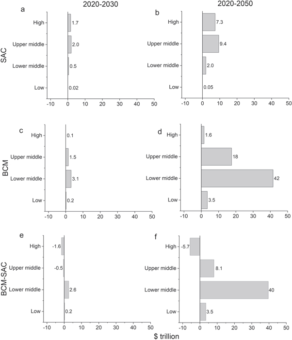
Figure 3. SACs and BCMs by income groups. (a) Income group-level total median SAC across IAM models for the 2020–2030 horizon. (c) Income group-level total BCM under SSP2 for the 2020–2030 horizon. (e) Income group-level total BCM (b) minus SAC (a) for the 2020–2030 horizon. (b), (d), (f). Same as panels (a), (c), (e) for the 2020–2050 horizon.
Download figure:
Standard image High-resolution imageFinally, we examine when contemporaneous annual (non-discounted) net benefits become positive over the 2020–2050 horizon, or the payback period. At the global level, the payback period for total net benefit is 5 years (figure 4(a)). Payback periods, however, vary substantially by income groups, consistent with income heterogeneity in total discounted net benefits. For lower-middle and low income countries, the payback period is 1 year (figures 4(d) and (c)). For upper-middle income countries, the payback period is 11 years. While for high income countries, payback never occurs (figure 4(b)).

Figure 4. Payback periods. (a) Annual (undiscounted) net benefit under median, minimum, and maximum SAC across IAM models and SSP2. (b)–(e) Reproduces panel (a) but separately for high, upper-middle, lower-middle, and low income country groups.
Download figure:
Standard image High-resolution image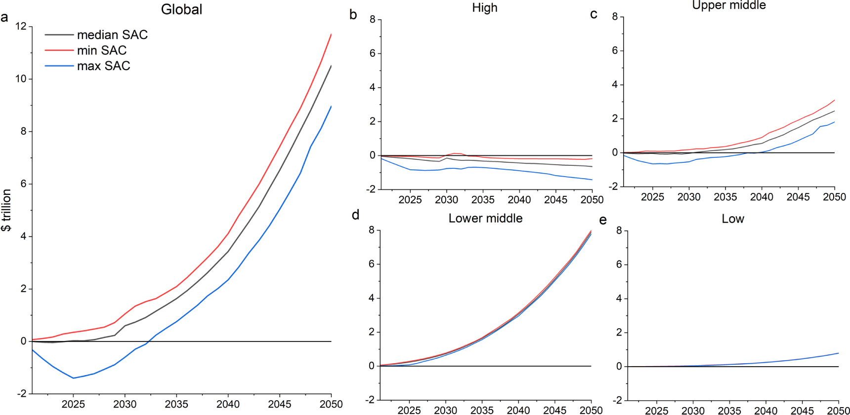
We subject our results to various additional sensitivity analyses by further adding the cost of stranded fossil fuel infrastructure (figures S1–S2); replacing our 3% discount rate with a 5% discount rate (figures S3–S4); examining specific IAM outputs that differ, among other features, by their endogenous fossil fuel price paths (figures S5–S10), considering different SSPs (figures S11–S12). We also analyze the distribution of net benefits on a per capita basis (figure S12). These analyses reaffirm our main conclusions: while important in the next decade, BCMs, not SACs, largely determine the sign of a country's net benefit over a 2020–2050 horizon.
4. Discussion
Although SAC is only a component of a country's total climate policy costs, which themselves may not reflect the particular concentration of political interests that influence a country's climate policy, a large SAC may partly explain the reluctance to support climate policy by countries with substantial fossil fuel reserves. The unequal distribution of costs from stranded assets and climate mitigation benefits may also speak to arguments for climate policy based on historical cumulative GHG emissions and the fairness principle. Higher income countries are responsible for nearly 90% of historical cumulative emissions (figure. S13). However, compared to lower income countries, higher income countries may also receive lower net benefits from joining a global 2 °C target. For example, the SAC for Iran, Russia, and Australia overweigh their BCM. It is notable that the NDCs of these nations also fall short in meeting the 2 °C target under the Paris Agreement [37], despite their large cumulative historical emissions. By contrast, the NDCs submitted by Morocco, Ethiopia, Kenya and Philippines reflect more ambitious goals in greenhouse gas emissions despite their smaller historical cumulative emissions.
Future work can extend our analysis along several dimensions. First, our analysis assumes all fossil profits accrue to a country. While 90% of reserves are indeed owned by countries, some of the total profits from fossil fuels may accrue to foreign operating companies that extract the fuel, affecting the distribution of SAC across countries [38]. Second, our SAC measure does not include the cost of stranded fossil fuel infrastructure, provided that this cost is not sunk. Although there are studies that quantify the stranded infrastructure cost of coal power plants [39–41], it is unknown how much of the other fossil fuel infrastructure (e.g., oil wells, refineries, and pipelines) will be stranded globally under a global 2 °C target. As a robustness check, we added stranded infrastructure cost into our SAC measure by assuming energy companies lose all their infrastructure assets (figures S1–S2). We find that adding infrastructure cost does not qualitatively change the overall spatial pattern of net benefits across countries.
Finally, as noted already, many other political and social determinants affect a country's adoption of climate policy besides economic costs and benefits. For example, decarbonization policies that target new capital stocks in the energy sector may help offset stranded asset costs, reshaping the influence of fossil fuels in global climate negotiations [42]. Likewise, policies that alter political access should also be considered as fossil fuel companies with high SACs may be more effective in lobbying over climate policies, undermining such policies' benefits to society [43]. Other social impacts of the climate policy, e.g., the unemployment from the stranded fossil fuel reserves, also play an important role in the design of a climate policy [44].
Even within an economic perspective, our measure of SAC and BCM misses important components of total costs and benefits. On the cost side, this includes how climate policy alters profits for non-fossil fuel producers and welfare for consumers. On the benefits side, this includes everything omitted from GDP, which notably includes potential health benefits of climate policy [45]. Furthermore, even within our narrow SAC measure, there are nuances to whether a high SAC necessarily implies opposition to particular forms of climate policy. For example, a fossil fuel-rich country with high benefits from climate policy may nonetheless support climate policy that favors carbon capture and storage technology which enables reduced net GHG emissions with continued fossil fuel production. Future research should incorporate how the results from this study along with these other considerations alter the prospects of international climate policy cooperation.
Acknowledgments
We acknowledge the Chancellor's Fellowship from the University of California, Santa Barbara. We appreciate the helpful feedback from Jing Meng, Yang Qiu and Jiajia Zheng.
Data availability statement
All data that support the findings of this study are included within the article (and any supplementary files).
Competing interests
The authors declare no competing interests.
Supporting information (5.2 MB DOCX)
source data for figures (3.5 MB XLSX)