ABSTRACT
We propose a generalization of Becker's cloud model (BCM): an embedded cloud model (ECM)—for the inversion of the core of the Hα line spectrum of a plasma feature either lying high above the forest of chromospheric features or partly embedded in the outermost part of this forest. The fundamental assumption of the ECM is that the background light incident on the bottom of the feature from below is equal to the ensemble-average light at the same height. This light is related to the observed ensemble-average light via the radiative transfer that is described by the four parameters newly introduced in addition to the original four parameters of the BCM. Three of these new parameters are independently determined from the observed rms contrast profile of the ensemble. We use the constrained χ2 fitting technique to determine the five free parameters. We find that the ECM leads to the fairly good fitting of the observed line profiles and the reasonable inference of physical parameters in quiet regions where the BCM cannot. Our first application of this model to a quiet region of the Sun indicates that the model can produce the complete velocity map and Doppler width map of the region.
Export citation and abstract BibTeX RIS
1. INTRODUCTION
The Sun seen through the core of the Hα line displays a variety of plasma features that appear in absorption against the solar disk. The best-known examples are filaments and mottles in quiet regions and fibrils, arch filaments, and surges in active regions. These features lie high above the forest of other chromospheric features and scatter the Hα light incident on them, like clouds in the sky of the Earth.
The cloud model (Beckers 1964) describes the effect of a cloud-like feature on the radiative transfer of the Hα line. This model of spectral inversion yields the values of the four parameters: Doppler shift, Doppler width, optical thickness, and source function. It is simple and hence has been frequently used in various features such as dark mottles (Grossmann-Doerth & von Uexküll 1971, 1973; Bray 1973; Tsiropoula & Schmieder 1997), as recently reviewed by Tziotziou (2007). Beckers' cloud model (hereafter BCM) has been generalized into several variants such as the variable-source-function cloud models (Mein et al. 1996; Tsiropoula et al. 1999), differential cloud models (Mein & Mein 1988), and multi-cloud models (Heinzel & Schmieder 1994; Gu et al. 1996; Chae et al. 2007).
In some chromospheric features, however, the BCM as well as the other variants of the cloud model breaks down. Grossmann-Doerth & von Uexküll (1973, 1977) found that the contrast profiles of network features are usually fitted by the BCM, which they categorized into the cloud or C-type, but most contrast profile in internetwork regions cannot. The cloud-type contrast profiles appear in absorption at all wavelengths or, if any, in emission near the core only. The other contrast profiles of showing emission in the wings, which were categorized into the X-type, cannot be fitted by the BCM. A good example is Hα dark grains, small dot-like features in internetwork regions that appear dark in the blue wing of the Hα line (Beckers 1968). In the red wing, however, they usually appear in emission against the background (Lee et al. 2000), which cannot be described by the BCM. Such contrast profiles with wing emission often occur in network regions and active regions as well, which may be the reason why the maps of BCM parameters have been presented in the incomplete form (e.g., Alissandrakis et al. 1990; Tsiropoula et al. 1993).
It is very likely that the contrast profiles with wing emission originate from low-lying features embedded in the chromospheric forest. By solving the non-LTE equation of radiative transfer with constant absorption profile, Durrant (1975) found that low-lying features display contrast profiles with both emission and absorption, while high-lying features show absorption only. This theoretical result is consistent with the earlier observations of Bray (1969) indicating that bright mottles are phenomena of the lower (≲3300 km) chromosphere while dark mottles are those of the upper (5000–7600 km) chromosphere.
The recognition that the BCM fails to account for contrast profiles of low-lying features showing wing emission led Steinitz et al. (1977) to introduce a new model of the contrast profile called an embedded feature model. This model is independent of the cloud model and attributes the emission characteristic to the difference in the optical thickness profile between the feature and the surrounding undisturbed atmosphere. By introducing the ratios of Doppler width and absorption strength and the optical thickness of the background atmosphere, the model successfully produced a variety of theoretical contrast profiles, including the one with absorption at all wavelengths, the one with core emission, the one with wing emission, and so on. Regrettably, however, this model was never applied to real observations as far as we know.
We propose an embedded cloud model (ECM), which is a generalization of the BCM. An embedded cloud in our model refers to a cloud-like structure of plasma the bottom of which is rooted in the upper chromosphere. The implicit but critical assumption of the BCM is that the profile of background light incident on the feature of interest from below is the same as the reference intensity profile which is usually taken by averaging many spectral profiles over the reference regions. This assumption is based on the belief that the bottom side of the feature lies higher than these reference regions, and the space between the feature and the reference regions is transparent to the light. In embedded clouds, however, the first condition above is not satisfied, and hence, the background intensity profile may differ from the reference profile. The essence of the ECM is to relate the two profiles using the radiative transfer of the ensemble average light as we shall show. The ECM is applicable to features in the upper chromosphere. This outermost layer mainly affects the core part of the Hα line with its vertical extent varying from feature to feature.
Our paper is organized as follows. In Section 2, we describe the spectral data to be used, and four representative chromospheric features seen in the data: two network features and two internetwork features. The methods of the spectral inversion are given in Section 3 together with the illustration using the four selected features. It is shown that the BCM is inadequate in some features, and then the formulation of the ECM is presented as well as the implementation of the model fitting. In Section 4, we apply the new technique of the spectral inversion to the whole area of the observed quiet region to produce its maps of optical thickness, line-of-sight velocity, Doppler width, source function, and so on. Based on the analysis of these maps, we discuss the characteristics of the ECM and deal with some critical issues.
2. OBSERVATION
The observation was done with the Fast Imaging Solar Spectrograph (FISS) of the 1.6 m New Solar Telescope at Big Bear Solar Observatory. The FISS is a dual band Echélle spectrograph that can record high resolution spectra of the Hα line and the Ca ii 854.2 nm on two different cameras simultaneously (Chae et al. 2013a). It does imaging by the fast scanning of the slit over the field of view. The early-run performance of the FISS as well as basic data processing is described by Chae et al. (2013a).
With the FISS, we observed a small quiet region on 2011 July 13. This set of data was previously used by Chae et al. (2013b) for the study of Doppler shifts in the quiet Sun. Only the Hα line data are used in the present work. Each Hα spectrogram (slit image) consists of 256 spectral profiles that represent the spatial variation along the slit with sampling of 0 16, and each spectral profile, of 512 data points that cover 0.97 nm (9.7 Å) with sampling of 1.9 pm (19 mÅ). The net spectral resolution was estimated to be 4.5 pm (45 mÅ) by Chae et al. (2013a). The position of the slit on the image plane was successively shifted with step size of 016, and one raster scan comprising 100 steps covered a 16'' × 41'' area inside the field of view. The raster scan was repeated every 18 s for half an hour.
We specifically define a spectral feature as the plasma structure emitting the light with Iλ, obs that is different from the reference line profile Rλ, obs. The observed contrast profile of a feature defined by

hence is to have non-zero values at least at some wavelengths. According to this definition, practically every observed contrast profile turns out to correspond to a feature.
Reasonably constructing the reference profile Rλ, obs from the observation is an important step for data fitting. Generally speaking, for each Iλ, obs, all the spectral profiles satisfying the priorly specified criteria are assembled into the reference ensemble, the set of all the profiles selected for the reference. The average of this reference ensemble is naturally adopted as the reference profile Rλ, obs. In principle, the reference ensemble and the reference profile can be constructed for every Iλ, obs, which is very time-consuming when the number of the observed profiles is big.
To save the computing time, we adopt a simple method in the present work. We form the reference ensemble and the reference profile using all the spectral profiles in internetwork regions (free from prominent network features), as in previous works (e.g., Grossmann-Doerth & von Uexküll 1973). This is done only once. For each Iλ, obs, this reference profile is slightly adjusted with a constant multiplication factor so that the contrast vanishes at the far wings and continua. This multiplication factor is very close to unity, so its effect on the contrast is insignificant in the core that is of our interest.
Figure 1 presents a set of monochromatic maps of the observed region constructed at several wavelengths of the Hα line and some examples of Iλ, obs, Rλ, obs and Dλ. Even though small, the observed area displays both the network region and the internetwork region. We have selected four features for demonstration. Features 1 and 2 are network features and features 3 and 4 are internetwork ones.

Figure 1. Top: monochromatic maps of a small quiet region constructed at the wavelengths of −400, −80, −40,0, +40, +80 pm measured from the center of the Hα line. Middle: Hα line intensity profiles of the four features (1–4 from left to right). The green symbols are the observed line profiles of the features of interest, and the blue curves are the corresponding reference profiles. Bottom: contrast profiles of the features against the corresponding reference profiles.
Download figure:
Standard image High-resolution imageFeature 1 represents a fine mottle a little away from the center of the rosette. It appears in absorption at every wavelength. This corresponds to the C-type contrast of Grossmann-Doerth & von Uexküll (1977). Feature 2 is located near bright network points in the rosette center. It appears in strong absorption at the red wing but in emission in the core. Thus, this is neither a dark mottle nor a bright mottle, illustrating that bright mottles and dark mottles are not clearly separable from each other (Grossmann-Doerth & von Uexküll 1973). This contrast profile is similar to the X3 type of Grossmann-Doerth & von Uexküll (1977).
Feature 3 in the internetwork region is a good example of an Hα grain. According to Beckers (1968), grains are small dots that appear in the blue wing of the Hα line. They have been thought to be the Hα counterpart of bright Caii K2V cell grains which in turn is related to the passage of a shock (Rutten & Uitenbroek 1991). This Hα grain appears in absorption at the blue wing but in emission at the red wing (similar to X1 type). Feature 4 does not have any special name. As far as we know, there is no report of this kind of feature. We think that it may represent a specific phase of the three-minute oscillation or the passage of a shock prevailing in the internetwork regions. This feature appears in emission at all the wavelengths (similar to X8).
3. METHOD
3.1. Beckers' Cloud Model
We here review the formulation of the BCM because it is the basis of the ECM we propose. The absorption profile is assumed to be uniform inside the feature and to be subject to Doppler broadening only. Then the optical thickness profile is given by
where τ0 is the peak absorption optical thickness, λ1 is the peak absorption wavelength of the profile related to the line-of-sight velocity v and the rest wavelength λ0 via
and W is the Doppler width
that is determined by the temperature T, the speed of non-thermal motion or microturbulence ξ, and the atomic mass of the line-emitting element M. The source function S is assumed to be constant over wavelength and position inside the feature. The constancy of S over wavelength is a general property of lines formed under the complete frequency redistribution. The observed intensity profile of the line emergent out of the feature Iλ, obs is then determined by the intensity of light incident on the feature from the opposite side Iλ, in as well as S and τλ

With this solution, the contrast profile defined by

is modeled like

This BCM has four free parameters: S, τ0, λ1, and W.
The remaining question is how to reasonably specify Iλ, in. As mentioned above, the BCM usually adopts the assumption

as illustrated in Figure 2, which leads to the equality  . Even though not explicitly made, this assumption is a crucial component of the model, being applicable to features lying high above the chromospheric forest. The success of the cloud model often depends on the plausibility of this assumption.
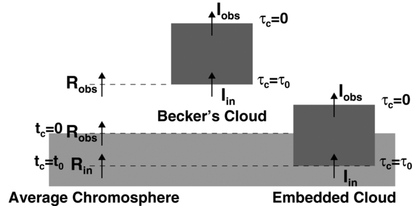
Figure 2. Illustrative drawing of the BCM and the ECM. The average chromosphere (or the chromospheric forest) is presented in light gray color and the features—a Becker's cloud and an embedded cloud—in dark gray color.
Download figure:
Standard image High-resolution imageFigure 3 shows the fitting of the BCM to the Hα spectral data of the four features, respectively. Note that the specific method of model fitting is described in Section 3.3. This model satisfactorily fits the Hα profile of feature 1 that appear in absorption at all the wavelengths against the reference, but fails to fit those of the other features that appear in emission at some wavelengths. The model profile looks similar to the observed profile of feature 2 but is not satisfactory at all. The fitting of features 3 and 4 are even worse.
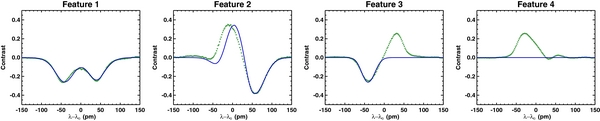
Figure 3. Hα contrast profiles (green) of the four features (1, ⋅⋅⋅, 4 from left to right) fitted by the BCM (blue).
Download figure:
Standard image High-resolution imageThis failure originates from the fact that the BCM rules out emission at wavelengths away from the center (Grossmann-Doerth & von Uexküll 1971). This can be easily understood with the help of Equation (7). The contrast Cλ becomes positive when S exceeds Rλ, in. In the upper chromosphere, however, S is usually lower than the minimum value of Iλ, in at the line center. Therefore, Cλ turns out to be usually negative. S can be larger than the minimum value of Iλ, in in some cases but still remains lower than the values of Iλ, in at wavelengths off the line center. This means that if there is any emission, it is likely to appear near the line center only, and not at off-center wavelengths.
3.2. Embedded Cloud Model
We have realized that the failure of the BCM should be attributed to the inadequacy of the assumption Equation (8). As already noted, this assumption easily breaks down when the feature of interest does not lie high above the reference features, especially when the feature of interest is embedded in the chromospheric forest (see Figure 2). Hence we propose to replace the assumption by a new one which holds in more general,

where Rλ, in is the average intensity of light at the same atmospheric height as Iλ, in. Note that Iλ, obs and Rλ, obs are observable, but Iλ, in and Rλ, in are not.
To relate the non-observable Rλ, in to the observed reference profile Rλ, obs, we formulate the radiative transfer for the ensemble average light in the following way. We first consider the radiative transfer along each ray, indexed by k, in the reference ensemble as expressed in

and
that have the same form as Equations (5) and (2). Introducing the ensemble-average quantities:

and defining tλ as in
we can reduce the ensemble average of Equation (10) to the form

For the tractability of the model, we adopt the assumption that tλ depends on λ in the same form as Equation (2)
with the three new parameters: t0, λ2, and w.
Note that the observed contrast profile Dλ defined in Equation (1) is now distinct from Cλ defined in Equation (6) because  any longer. Combining Equations (1), (5), (9), and (14), we obtain the ECM equation of the observed contrast profile

with the abbreviations Δτλ ≡ τλ − tλ and ΔS ≡ S − s. This equation indicates that the non-zero contrast of a spectral feature is attributed to either Δτλ or ΔS. Note that positive Δτλ leads to negative contrast while positive value ΔS, to positive one. Note that in the limit tλ → 0, the ECM is reduced to the BCM.
3.3. Model Fitting
To determine the parameters, we use the constrained fitting of the model (Chae et al. 1998) that minimizes the functional

where the "reduced" chi-square χ2 defined as
is to make the model  as get close to the data
  as possible,—where N is the number of wavelength points and σD is the standard error of each data value—and the constraint Π defined as
is to regularize each parameter pj by constraining it to its default value pj, d within the extent defined by σ(pj), the standard deviation of pj from the default value. Note that in the limit σ(pj) → ∞ the parameter pj behaves as an unconstrained free parameter independent of the default value, and in the other limit σ(pj) → 0, as a fixed parameter equal to the default value. By adopting an appropriate value of σ(pj) in the intermediate range, we can also constrain pj to the default value either loosely or tightly.
The ECM has eight parameters: τ0, λ1, W, S, t0, λ2, w, and s. Among these, we regard the four parameters τ0, λ1, W, S only as unconstrained free parameters, and t0 as a free parameter loosely constrained to 0 with σ(t0) = 1. We fix the other parameters λ2, w, and s to the default values: −1.8 pm, 35 pm, and 0.12Ic, which we obtained from the analysis of root-mean-square (rms) contrast profiles of intensity in the reference ensemble as described in Appendix A.
Our model fitting consists of three stages. First, we construct a number of model profiles  for every set of parameters in the parameter space. In this space, each of [τ0, W, S, t0] has five different values, and λ1 have 11 different values, the other parameters are fixed to the default values, so the total number of synthetic profiles in the archive is 6875. Next, the observed contrast profile is compared with all of these profiles in the archive, and the closest matching profile is selected, and the parameter values of this selected profile is used as the initial guess for the nonlinear least-square fitting. Finally, the iteration of the parameters is done with the Marquardt's gradient-expansion algorithm that is implemented in the standard procedure curvefit" of the Interactive Data Language.
The value of σD needs to be specified for the calculation of χ2. The smaller σD is, the bigger χ2 is. After a few trials, we have adopted a value for σD ensuring that the median of χ2 values in the observed quiet region is close to 1. Then, with this choice of σD, χ2 = 1 represents a typical goodness of fitting in the quiet region.
4. RESULTS
4.1. Examples
The top panels of Figure 4 show the result of the ECM fitting. We find that the new model fitting is no better than the BCM in feature 1. However, it is much better in feature 2 and is excellent in features 3 and 4. Note that the contrast profiles of features 3 and 4 cannot be fitted by the BCM at all (see Figure 3).

Figure 4. Top: Hα contrast profiles (green symbols) of the four features Dλ fitted by the ECM (red curves). Middle: variations of χ2 (blue), Π (red), and H (black) with t0. Each asterisk shows the values of t0 and χ2 at the H minimum. Bottom: profiles of Rλ, in (red) obtained from the model fitting compared with the profiles of Iλ, obs (green) and Rλ, obs (blue).
Download figure:
Standard image High-resolution imageThe strength of the new model originates from the newly introduced parameter t0. The uniqueness and role of this parameter in the model can be inferred from the plots of χ2 as a function of t0 presented in the middle panels of Figure 4. Note that with each given value of t0, the other parameters have been chosen to ensure the minimum of χ2, and the special case of t0 = 0 corresponds to the BCM.
There exist different patterns in the variation of χ2. In the case of feature 1, χ2 is fairly small for t0 = 0, slowly decreases with t0, and displays a shallow minimum at t0 > 1. The profiles of this type can be adequately fitted by the BCM as well, and t0 of the ECM remains ill-determined unless the constraint is used. The role of the imposed constraint Π is thus crucial in this type. It forces the minimum of H to occur at t0 as small as possible, making the solution be close enough to the BCM. The second type is well represented by the other features. In this type, χ2 at t0 = 0 is very big, implying the inadequacy of the BCM. The minimum occurs at t0 ∼ 1. If the minimum is deep (e.g., features 2 and 4), the effect of the constraint on the solution is minor. If not (e.g., feature 3), the constraint becomes significant, forcing t0 to be as small as possible.
The bottom panels of Figure 4 show the inferred Rλ, in in comparison with Rλ, obs and Iλ, obs. The bigger t0 is, the more Rλ, in deviates from Rλ, obs. Note that Rλ, in is higher than Iλ, obs at every wavelength in all the features. It implies that with the choice of  , Cλ is negative at all the wavelengths and can be well fitted by the BCM. We also note that a big value of t0 is not preferred. If t0 is too big, then Rλ, in deviates too much from Rλ, obs and might deviate much from the real as well.
Table 1 presents the determined values of the parameters with their probable standard errors estimated using the bootstrap method. With these values, we can understand the emission/absorption characteristic seen in each contrast profile. The absorption at all the wavelengths in feature 1 is mostly due to Δτλ > 0. The emission in the red wing in feature 2 is the combined effect of ΔS > 0 and the large redshift of τλ that leads to Δτλ < 0 (hence emission) in the blue wing. The absorption/emission characteristic of feature 3 originates from the blueshift of τλ (upward moving plasma) causing Δτλ > 0 (hence absorption) in the blue wing and Δτλ < 0 (hence emission) in the red wing. Finally, the physical origin of emission characteristic of feature 4 is a little hard to understand. It appears that the emission characteristic is mainly due to W < w which leads to Δτλ < 0 at all the wavelengths. The redshift of τλ is in charge of the blue-red asymmetry; it causes the significant negative value of Δτλ (hence strong emission) in the blue wing, and the insignificant negative value of Δτλ (hence week emission) in the red wing.
Table 1. Parameters of the Embedded Cloud Model Determined from the Fitting
| Feature | τ0 | v | W | S/Ic | t0 | χ2 |
|---|---|---|---|---|---|---|
| (km s−1) | (pm) | |||||
| Feature 1 | 1.27 ± 0.13 | −1.1 ± 0.1 | 48.2 ± 1.1 | 0.13 ± 0.00 | 0.22 ± 0.19 | 1.30 |
| Feature 2 | 1.88 ± 0.10 | +8.9 ± 0.7 | 50.0 ± 0.9 | 0.18 ± 0.01 | 1.62 ± 0.14 | 3.61 |
| Feature 3 | 1.65 ± 0.17 | −8.2 ± 0.7 | 31.8 ± 0.8 | 0.12 ± 0.00 | 1.44 ± 0.12 | 0.91 |
| Feature 4 | 1.33 ± 0.13 | +4.4 ± 0.3 | 25.6 ± 0.3 | 0.16 ± 0.00 | 1.05 ± 0.05 | 0.32 |
Download table as: ASCIITypeset image
4.2. Parameters of the Observed Region
The ECM is superior to the BCM in that it can produce the complete parameter maps of the observed region on the quiet Sun as is demonstrated in Figure 5. Thanks to the flexibility associated with a new free parameter t0, the ECM can be applied not only to network features, but also to internetwork features, and hence to all the quiet region features. The χ2 map indicates that the ECM fit is excellent in the internetwork region. In the network region, χ2 is bigger, but the goodness of fit is still satisfactory at most points as illustrated in the fits of features 1 and 2 (see Figure 4). These fits are no worse than any of cloud model fits published so far, e.g., Figure 4 of Grossmann-Doerth & von Uexküll (1971) and Figure 2 of Tsiropoula et al. (1999).
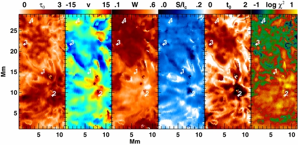
Figure 5. Parameter maps of the observed region.
Download figure:
Standard image High-resolution imageIn contrast, recalling that the ECM in the limit t0 → 0 is reduced to the BCM, we find from Figure 5 that the applicability of the BCM is limited. The white-colored (t0 = 0) area of t0-map where the BCM is applicable excludes most of the internetwork region and a significant portion of the area near the center of the rosette structure. This limited applicability of the BCM explains why the maps of parameters in a rosette previously obtained using the BCM (e.g., Tsiropoula et al. 1993) were left unfilled in many places.
Figure 5 shows a few spatial patterns of the parameters. First, the central part of the rosette is redshifted whereas its outer part is blueshifted. Even inside an individual fibril (say the one including feature 1, the inner (or lower) part is redshifted, and the outer (upper) part, blueshifted, which confirms the earlier studies (e.g., Tsiropoula et al. 1993). Second, bright mottles and dark mottles are distinguished by the source function, quite in line with the previous study of Bray (1973) and Heinzel & Schmieder (1994). In addition, the different appearance of dark mottle contrast in the red wing and blue wing is due to the Doppler shift. Finally, W in the network region is systematically larger than in the internetwork region, confirming the result of Cauzzi et al. (2009). In fact, we find from Figure 6 that the number distribution of W in the quiet region is bimodal. The peak around 30 pm represents the internetwork region, and the one around 46 pm the network region. If ξ does not differ much between these regions, the difference in W reflects difference in T. With the choice of, for example, ξ = 8 km s−1, these Doppler widths yield the estimates T = 7500 K and 23,000 K, respectively.
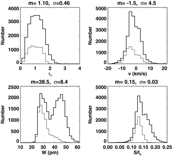
Figure 6. Number distributions of the ECM parameters in the quiet region. The top of each plot indicates the mean and standard deviation. Thin histograms represent the number distributions in the internetwork region.
Download figure:
Standard image High-resolution imageFigure 7 compares the inferred line-of-sight velocities between the lambdameter method and the ECM method. The lambdameter method fits a horizontal chord (lambdameter) of width 2Δλ into the observed line profile. The wavelength corresponding to the center of the lambdameter is adopted as the measured wavelength of the line, and hence a measure of Doppler shift. Since this method works without failure as long as the Hα line appears in absorption, it has been often used to produce the complete Doppler shift map of the observed region (e.g., Chae et al. 2013b). As expected, the figure shows that the ECM velocities are strongly correlated with the lambdameter velocities. The Peterson coefficient is found to be 0.87. Note, however, that there is a big difference in velocity magnitude between the two methods: the standard deviation of the lambdameter velocities is 1.3 km s−1 and that of the ECM velocities, 4.5 km s−1. Supposing that the ECM velocities are close to the real, we find that the lambdameter velocities are seriously underestimated, on average, by a factor of 3 to 4, which was well-known from previous studies (e.g., Alissandrakis et al. 1990; Tsiropoula et al. 1993). More serious is that despite the strong correlation, the one-to-one correspondence between lambdameter velocities and the ECM velocities is far from unique. For example, the lambdameter velocity of 2 km s−1 corresponds not to a single value of the ECM velocity but to its broad range from 3 km s−1 to 15 km s−1.
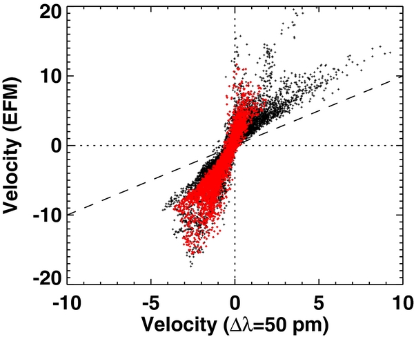
Figure 7. Scatter plot of line-of-sight velocity determined with the lambdameter method (Δλ = 50 pm) and velocity determined with the ECM. The black dots are from the network region, and the red ones are from the internetwork region.
Download figure:
Standard image High-resolution image5. DISCUSSION
5.1. Characteristics of the ECM
We have introduced the ECM for the spectral inversion of the Hα line for a plasma feature in the upper layer of the chromosphere. Like the Beckes' cloud model (BCM), the ECM assumes that the absorption profile (characterized by Doppler width W and line-of-sight velocity v) and the source function S are uniform inside the feature of optical thickness τ0. The ECM, however, differs from the BCM in the way of adopting Iλ, in. As illustrated in Figure 2, Iλ, in is identified with Rλ, obs in the BCM, but it is identified with Rλ, in in the ECM. We have proposed to relate between Rλ, obs and Rλ, in via the radiative transfer of ensemble-average light across the average chromospheric layer, which is parameterized by optical thickness t0, source function s and Doppler width w. The ECM has practically one additional free parameter t0 with the other additional parameters being either fixed or tightly constrained to the default values. With the flexibility associated with t0, the ECM can fit all the intensity profiles of the observed quiet region and produce the complete maps of line-of-sight velocity, Doppler width, optical thickness, source function, and so on.
In determining line-of-sight velocity the ECM is superior either to the lambdameter method or to the BCM in two aspects. The lambdameter method can give us some qualitative information such as the spatial distribution of redshift and blueshift, but cannot produce reasonable velocities for a quantitative analysis. For this purpose, the BCM is preferred to the lambdameter method. The BCM, however, is limited in its applicability; there are many regions where the BCM cannot be applied. The ECM has no such limitation; it can produce not only the complete velocity map of the observed region, but also it can produce reasonable velocity values suited for quantitative studies.
The critical parameter in the ECM, t0, has a clear physical meaning. It refers to the atmospheric level where the bottom of the feature is located. If t0 is much smaller than 1, the feature lies high above the chromospheric forest, like a cloud. If t0 becomes comparable to or larger than 1, the bottom of the feature is embedded inside the chromospheric forest. Thus, t0 provides us with some information on the geometric height. Roughly speaking, the feature with bigger t0 extends down to a deeper level than the one with smaller t0. By constraining t0 to be as small as possible, we aim to infer the physical parameters of features in the outer layer of the chromosphere.
Our ECM can be used to chromospheric features in other environments as well if the reference ensemble is well established. The reference ensemble we used in the present study consists of the spectral profiles extracted from the internetwork region. It provided us with the observed reference profile Rλ, obs and the default parameters of λ2, w, and s. With these data, the spectral profiles of the internetwork features were excellently fitted by the model. Those of the network features were fitted by the model a little worse than the internetwork features. We do not know the main reason for the degraded goodness of fitting in the network features, but we suspect that the poorer fitting may be partly because the reference ensemble is not from the network environment itself, but from the internetwork environment. Nevertheless, we think the radiation field may not be much different between the two environments because the model fitting of network features is still good enough. Each environment of active regions such as sunspot umbrae, sunspot penumbrae, and plages may be quite different from that of the quiet Sun. Therefore, it would not be reasonable to use Rλ, obs, λ2, w, and s obtained here for the study of features in the above environments, and it is necessary to establish a new set of these data for each environment.
The ECM may be compared with other variants of the cloud model introduced for the same purpose: to overcome the difficulty of finding the suitable Iλ, in. Assuming Iλ, in is symmetric, Liu & Ding (2001) applied the fitting to the profile of intensity difference between the blue side and the red one where Iλ, in disappears. This method is good when the observed line profile is significantly asymmetric so that it highly deviates from the supposed Iλ, in. Some asymmetric line profiles in the quiet region may be fitted with this method, but there are many features in the quiet Sun displaying line profiles that are little asymmetric, where the method is not effective. Another interesting approach is to adopt the theoretical reference profile constructed by using the non-LTE profile synthesis. Bostanci & Al Erdoğan (2010) found that the synthetic profile computed from the Kurucz radiative-equilibrium model is the best choice as Iλ, in for the cloud modeling of Hα features in the quiet Sun. With this choice almost all the profiles were fitted by the BCM, and the determined cloud model parameters were in good agreement with the VAL-C atmospheric model. This approach of Bostanci & Al Erdoğan (2010) is similar to the ECM in that it admits  , but it differs from the ECM in that it uses one synthetic profile as an input Iλ, in for all the features while the ECM uses Rλ, obs as an input for all the features and yields Iλ, in as an output for each individual feature.
5.2. Some Critical Issues
5.2.1. Can the Source Function be Assumed to be Constant Inside Each Embedded Cloud?
Like the BCM, the ECM assumes the constancy of the source function S inside the feature and in the ensemble average chromosphere, which is the basis of Equations (5) and (14). The assumption of constant S holds most satisfactorily in an optically thin homogeneous cloud lying high over the chromosphere where the BCM can be successfully applied. Generally speaking, however, S is likely to vary with position.
Since S of the Hα line is mostly determined by the angle-averaged mean intensity in the upper atmosphere, and the contribution of lateral illumination and hence the mean intensity increase with depth, it is likely that S increases with optical depth both inside the feature and in the average chromosphere. In fact, Mein et al. (1996)'s non-LTE models of a horizontal slab irradiated from below indicates that the source function increases with optical depth inside the slab in all the models, even for optically thin slab models. Mein et al. (1996) also suggested a variant of the cloud model which makes use of this result of model computations. The variation of S over optical depth is approximated by a quadratic function of optical depth the coefficients of which are fully specified by the optical thickness of the slab.
The variation of the source function in a stratified mean atmosphere can be inferred from the values of hydrogen population given in the Table 17 of Vernazza et al. (1981). Using Equation (A9), we have calculated s/Ic as a function of height in the VAL Model C, and found that at height ⩽2000 km, s/Ic monotonically increases with depth. A noticeable feature of the model is that s/Ic varies too slowly from 0.073 to 0.085 with depth at heights between 1400 and 2000 km, representing the upper chromosphere, so that it can be assumed constant (∼0.08) in this range.
Note that the ECM deals with not the whole chromosphere of large range of optical depth but with the embedded cloud and the outermost layer of the average chromosphere whose optical thickness in the Hα center is order of unity. We expect the variation of the source function within this range to be small enough to be well described by low order polynomials of optical depth. The approach we adopt in the present study is to keep only the lowest order term, that is, the constant term. If this choice of approximation leads to a successful reproduction of the observed spectral profiles, we can be satisfied with it; if the model too much deviates from the data, then we may have to make the model more sophisticated by including the first order term or even the second order term. In Appendix B, we have presented the generalization of the ECM that takes into account the first order term of the source function δS as well.
As a matter of fact, we have fitted the contrast profiles of the four features with this generalized ECM and compared the results with the ECM with a constant source function. In features 3 and 4, δS is practically zero, and there is no significant difference in the value of the parameters between the two models. In feature 1, the ECM with variable source function yields S/Ic = 0.14 and δS/Ic = 0.14, which are significantly different from the ECM with constant source function S/Ic = 0.13 and δS/Ic = 0. There is little difference, however, in the values of other parameters and χ2 between the two models. The biggest difference between the two models occurs in feature 2. As shown in Figure 8, the model with the variable source function (S/Ic = 0.28 and δS/Ic = 0.51) better fits the observed profile than the one with the constant source function S/Ic = 0.18. We find that the inclusion of the δS term in the model affected the value t0 the most, changing it from 1.6 to 0.90, and then the value of τ0, changing it from 1.9 to 2.1. The other parameters λ1 and W changed little. From these comparisons, we conclude that the ECM with the variable source function can better fit the observed line profiles at the network regions where the ECM fitting with constant source function is poorer.

Figure 8. Comparison of model fitting between the model with a constant source function (left) and the one with a variable source function (right) in feature 2.
Download figure:
Standard image High-resolution image5.2.2. Can the Incident Radiation be the Same at Every Point in the Lower Parts of the Features?
One assumption of the ECM is that Iλ, in is the same at every point in the horizontal plane tc = t0 as expressed in Figure 2 and Equation (9) or, practically speaking, Iλ, in varies much less in the horizontal plane than Iλ, obs does. This assumption is reasonable in a couple of ways. We first note that the specific form of Iλ, in originates from the low atmosphere tc > t0 while that of Iλ, obs is determined by the whole atmosphere tc > 0 that includes the above low atmosphere. As a consequence, the horizontal variation of Iλ, in reflects the inhomogeneity of the low atmosphere only, but that of Iλ, obs does not only this inhomogeneity but also the inhomogeneity of the outermost layer 0 < tc < t0. Moreover, the inhomogeneity of plasma increases with height in the solar atmosphere because the dynamic and thermal interaction of plasma across field lines is more and more inhibited as the plasma β decreases with height, and velocity fluctuation usually increases with height. Thus, the inhomogeneity of the outermost layer may be much stronger than that of the low atmosphere. As a matter of fact, observations indicate that the rms contrast of a quiet region is much bigger in the core—that mostly originates from the outermost layer of the atmosphere, rather than in the wings, which is what it does from the lower atmosphere (see Figure 9). For these reasons, we neglect the spatial variation of Iλ, in, and we set it equal to Rλ, in, which makes the model simple and tractable.

Figure 9. Observed rms contrast profile (green) of the reference ensemble Gλ and the model fitting (red).
Download figure:
Standard image High-resolution image
There is a situation, however, when the assumption  is not valid. For example, when more than one chromospheric feature lies along the line of sight, Iλ, in incident on the outermost feature originates not only from the low atmosphere but also from the other lower-lying chromospheric features, so that it differs much from Rλ, in inferred from Rλ, out of a large area of the internetwork region. In this case, the BCM appears to be a better choice since the average of the rays over a small local area nearby containing similar chromospheric features can be reasonably used as the background profile for the BCM.
5.2.3. How do We have to Interpret the Maps of Parameters?
The maps of model parameters shown in Figure 5 could be complete because all the profiles in the observed region were reasonably fitted by the ECM. But how do we have to interpret these maps? Roughly speaking, they show the two-dimensional distributions of the parameters in the upper chromosphere sensed through the line core. Note, however, that these maps are not displaying parameters at the same geometrical height; the bottom of the upper chromosphere, as measured by t0, in fact, varies from feature to feature in the observed region. This implied unevenness of the upper chromosphere is definitely an intrinsic property of the solar chromosphere, since it is not an artifact of a model.
5.2.4. How can the ECM Inversion be Compared with the Forward MHD and Non-LTE Modeling?
The forward modeling based on radiation-MHD simulations and three-dimensional non-LTE radiative transfer computations is very useful in understanding of the formation of the Hα line throughout the solar chromosphere. It can describe the variation of source function over height, specify the formation height for each wavelength, and provide synthetic line profiles that can be compared with, e.g., the average of the observed line profiles. The recent study of Leenaarts et al. (2012) provided a set of meaningful results based on the state-of-the-art forward modeling. It is particularly interesting that the simulation successfully reproduced chromospheric fibril-like structures in synthetic observables for the first time.
In contrast, the ECM inversion is intended to extract empirical information from data, that is, a large number of individually observed line profiles. The tractability crucial for the processing of large data in the inversion is achieved by adopting several simplifying assumptions. It then always remains a problem whether these assumptions are reasonably good or not. Moreover, the interpretation of the results of inversion should be also carefully done as we mentioned above.
The forward modeling is complementary to the ECM inversion, in that it is quite helpful in examining the assumptions of the ECM inversion and in interpreting the inversion results. For example, Figure 4 of Leenaarts et al. (2012) indicates that the source function is independent of local temperature and fairly uniform in the formation heights of the Hα line center. This supports the assumption of the constancy of the source function introduced for the ECM inversion. Leenaarts et al. (2012) also suggests that the formation height of the line core is between 1 Mm and 2 Mm above average optical depth unity at 500 nm, and varies much from region to region. This information should be taken into account in interpreting the results of the ECM inversion.
The ECM inversion can be complementary to the forward modeling as well. For example, the inversion provides empirical information on the velocity and temperature of plasmas in the upper chromosphere, and this information would serve as the reference data for the forward modeling. So far, the forward modeling itself has rarely been used to fit individual observed line profiles to infer the atmospheric structure.
6. CONCLUSION
It is encouraging that the ECM can satisfactorily fit most of observed Hα contrast profiles in the quiet Sun, particularly X-type contrast profiles in internetwork regions that cannot be fitted at all by the BCM (Grossmann-Doerth & von Uexküll 1973, 1977). The ECM inversion can be used to infer physical parameters of an individual feature in the outermost layer of the quiet chromosphere, such as line-of-sight velocity, Doppler width, and source function, as well as optical thickness. We expect the ECM to serve as a useful tool for the investigation of the physical property and dynamical processes of the upper chromosphere in the quiet Sun, particularly in internetwork regions. It will be interesting to investigate in the future whether and, if so, how the ECM can be applied to other spectral lines as well, such as the Ca ii line at 854.2 nm, and to other regions as well, such as sunspots and plage regions.
We are grateful to the referee for the careful reading of the manuscript and a number of constructive comments. This work was supported by the National Research Foundation of Korea (NRF-2011-0028102 and NRF-2012R1A2A1A03670387).
APPENDIX A: DETERMINATION OF λ2, w, s
Combining Equations (9), (10), and (14), we obtain the ECM equation of the observed contrast profile along each ray indexed by k in the reference ensemble
with the abbreviations  and ΔSk ≡ Sk − s. This equation is of the same form as Equation (16).
We determine the default values of λ2, w, and s from the rms contrast profile of the reference ensemble defined by
which is a spectrum of intensity fluctuation in the ensemble. With the above formulation, the intensity fluctuation is attributed to the variations of the parameters— ,
,  , Wk, and Sk—inside the ensemble as well as due to a statistical noise σ0. Supposing that the ensemble averages of these parameters are equal to t0, λ2, w, and s, and their deviations from these averages are small, we can apply a linear analysis of perturbation propagation to obtain the increments


and Gλ
where
The model of Equation (A5) is to be fitted with nine parameters: λ2, w, s, t0,  , σ(λ1), σ(Wk), σ(Sk), and σ0. The careful examination of Equation (A5) reveals that the dependence of the model on t0 appears only in t0σ(λ1), t0σ(Wk), and [1 − exp (− tλ)]σ(Sk). Under the approximation 1 − exp (− tλ) ≈ tλ, this last term also turns out to be proportional to t0σ(Sk). Therefore, under the assumption of small t0, the model practically has eight free parameters: λ2, w, s,
  , t0σ(λ1), t0σ(Wk), t0σ(Sk), and σ0, among which only the first three parameters are needed for the fitting of Equation (16).
Figure 9 shows the rms contrast profiles of Gλ constructed from the reference ensemble representing the internetwork region. This rms contrast profile is very similar to the one reported by Grossmann-Doerth & von Uexküll (1973) in shape, but its peak value 0.13 is higher than the old measurement 0.09. We find that the model fitting is excellent. The inferred parameters are λ2 = −1.8 pm, w = 0.35 pm, s = 0.12Ic,  , t0σ(λ1) = 6.9 pm, t0σ(Wk) = 1.1 pm, t0σ(Sk) = 0.007Ic, and σ0 = 0.066Ic, respectively, where Ic is the intensity of the continuum near the Hα line at the disk center.
The inferred value of s/Ic = 0.12 can be compared with the table of level populations of the VAL Model C (Vernazza et al. 1981). Note that the value is directly related to the value of n3/n2 via the equation
where n2 and n3 are the density of n = 2 and n = 3 level population of neutral hydrogen, respectively, g2 and g3 are the statistical weights, and Tc = 6100 K is the color temperature of the continuum. Table 17 of Vernazza et al. (1981) indicates that n3/n2 ranges from 0.0047 to 0.011 in the heights from 2090 to 2200 km—where T increases from 8440 K to 24,000 K, resulting in s/Ic = 0.074 to 0.17. The height where the VAL Model C produces the value of s/Ic the closest to the inferred value is 2115 km where T = 21, 000 K. We conclude that the inferred value of s/Ic is consistent with the physical condition of the outermost chromospheric layer of the VAL Model C.
APPENDIX B: THE ECM WITH A VARIABLE SOURCE FUNCTION
We allow the source function to vary inside the cloud but not in the background chromosphere. The simplest form of a variable source function is a first order polynomial of optical depth. We denote the average value of the source function inside the cloud by S, and its variation across the cloud by δS: S − δS/2 at the top and S + δS/2 at the bottom. The effect of non-zero δS can be incorporated into the ECM by adding to the right hand side of Equation (16) a new term that is proportional to δS as follows: