
Abstract
The description of the lateral resolution criterion for profile and areal surface topography measuring instruments is still under discussion in the international standardization. Several studies have examined the different methods proposed in the standardization individually. We describe a comprehensive examination and comparison of the different methods proposed by the standard. In doing so, the star-shaped grooves material measure (type ASG of ISO 25178-70) and the chirped standard are compared by using different measuring instruments and principles. In order to benchmark the results, they are compared to a third method for the transfer function determination which uses an Rk-calibrated material measure and is based on time series modeling. The results illustrate that both described methods have their specific advantages and disadvantages and are well-suited for individual fields of application.
Export citation and abstract BibTeX RIS

Original content from this work may be used under the terms of the Creative Commons Attribution 3.0 licence. Any further distribution of this work must maintain attribution to the author(s) and the title of the work, journal citation and DOI.
1. Introduction and state of the art
Describing the resolution limit can be important for the benchmarking of surface topography measuring instruments. This property is one metrological characteristic that can assist in describing the capabilities of measuring instruments [1]. The determination of the metrological characteristics is the foundation for the calibration of surface topography measuring instruments. The calibration of areal surface topography measuring instruments is not yet standardized, however, an according standard is currently under preparation [2]. Besides the already available standards for material measures [3] and the metrological characteristics [1], the −700 series of ISO 25178-700 will be the third pillar for the calibration of topography measuring instruments.
Because the general transfer characteristics of a measuring instrument contain important information, their determination has been extensively researched. Foreman et al provided a detailed overview considering the transfer function determination [4].
A measurement is for example possible with a rectangular grating [5], the chirped standard [6, 7] or the super-fine roughness standards [8]. The author proposed a calibration artifact that was specifically designed to image certain frequency-dependent properties for a calibration of transfer properties [9]. Su et al used a small sphere for the determination of transfer functions [10]. Leach et al give an overview of samples which have been utilized to measure the transfer characteristics [11].
Besides the measurement of transfer properties, virtual measurements have been examined for their determination [12–15]. Also the determination based on theoretical models like the instrument transfer function have been proposed [16, 17]. Yashchuck et al used a pseudo-random grating for the measurement of the modulation transfer function [18].
Also the current ISO standardization addresses the topic of transfer characteristics estimation. The ISO 25178-600 series proposes multiple approaches: firstly, the response function of an axis can be determined [1] which is usually characterized by the amplification coefficient and linearity deviation of the corresponding axis and can be measured for example with step height artifacts or gratings [19].
Additionally, to determine the frequency-dependent properties of an axis, there are several ways to determine the lateral resolution limit based on the topography fidelity and the topographic spatial resolution [1]. Although the basic concepts are universally applicable, for the evaluation of each of the two criteria there is as well at least one corresponding material measure: the Siemens Star or star-shaped grooves material measure (Type ASG) in ISO 25178-70 provides a measure that corresponds with the lateral period limit [20, 21]. The concept of the topography fidelity is generally applicable for arbitrary target geometries. However, in practice the chirped standard [6] has been proposed and examined for the evaluation of this criterion [22].
Both approaches have advantages: the measurement and evaluation of the chirped standard is applicable and comparable for different measuring principles, whereas the type ASG material measure allows a stepless calibration. The utilization of the two material measures for itself has been examined previously. The objective of our study is a systematic and comprehensive comparison of the two methods. Additionally, the measured results for the transfer functions are compared towards a model-based approach which is based on a time series description [23].
2. Experimental setup
In order to perform a comprehensive description of the lateral resolution limit determination, four different instruments were used. Table 1 gives an overview regarding the different utilized measuring principles.
Table 1. Utilized measuring principles for the described study.
| No. | Measuring principle | Resulting topography |
|---|---|---|
| 1 | Confocal Microscope (CM) | Areal |
| 2 | White Light Interferometer (WLI) | Areal |
| 3 | Stylus Instrument (SI) | Profile |
| 4 | Chromatic Confocal Microscope (CCM) | Profile |
The devices were applied to determine their transfer behavior or their lateral resolution limit respectively. In doing so, four different samples were used that were manufactured with two different methods:
- (1)As a first examination, Siemens Stars (ASG) in different scales that were manufactured with the aid of direct laser writing (DLW) (see [24, 25]) were measured with all areal instruments in different configurations. In previous examinations, it was possible to show that this additive manufacturing technology [26] is a suitable approach for the manufacturing of profile and areal material measures [24, 25, 27, 28]. Figure 1(a) illustrates an example of direct laser written material measures. In the microscope image different samples that feature a size of 100 μm × 100 μm each are shown which illustrate the capabilities of the manufacturing principle to reliably generate different topographic structures in the micrometre-range. The examined Siemens Stars have sizes of 100 μm × 100 μm, 200 μm × 200 μm, 400 μm × 400 μm and 800 μm × 800 μm and feature 16 pairs of petals with a nominal step height of 3 μm. The samples are made out of a polymer that is coated with a 30 nm layer of Iridium in order to enhance their reflectivity [25].
- (2)
- (3)A well-known method for the manufacturing of profile material measures is the application of ultra-precision turning [9, 29]. Thus, another chirped standard that was manufactured from brass (CuZn40Pb2) with this method was additionally examined. The chirped profile features a nominal amplitude of 400 nm which is decreased for shorter wavelengths in order to enable the mapping of these high spatial frequencies with the applied tool geometry. This second chirped standard (CIN-UPT) that was manufactured with the use of ultra-precision turning features a wider set of wavelengths than the previously mentioned DLW samples [23]. Figure 1(b) illustrates a typical material measure which was manufactured with the method of ultra-precision turning. With this technology, deterministic rough patterns can be imaged onto a surface.
- (4)The Rk-standard (RKS) is the fourth examined type of sample and represents an actual component surface and is used to characterize the measurement of functional surface characteristics [30]. In previous examinations it was demonstrated that this specific geometry can describe the transfer behaviour of different measuring instruments precisely based on time series modeling [23]. The examined sample was manufactured by ultra-precision turning of a nickel-phosphorus coated workpiece.

Figure 1. Examples for the manufacturing of material measures with direct laser writing (a) and with ultra-precision turning (b).
Download figure:
Standard image High-resolution imageThe instruments CM and WLI were applied with different magnification values leading to the set of measurements described in table 2. In order to benchmark the evaluated transfer properties according to the ISO 25178-600 series [1], the determined transfer functions based on the Rk-standard were used. All measurements with the confocal microscope were evaluated with a centre-of-gravity evaluation in order to determine the measured topography height values. The WLI features a Mirau configuration and the topography height values were calculated with a phase-evaluation.
Table 2. Overview of the measurements of the samples (a)–(d) with the described instruments (1)–(4).
| Measuring setup | (a) ASG | (b) CIN-DLW | (c) CIN-UPT | (d) RKS |
|---|---|---|---|---|
| 1(a) CM 20× NA = 0.45 | x | x | x | x |
| 1(b) CM 50×, NA = 0.5 | x | x | x | x |
| 1(c) CM 100×, NA = 0.95 | x | x | x | x |
| 2(a) WLI 20×, NA = 0.4 | x | x | x | x |
| 2(b) WLI 50×, NA = 0.55 | x | x | x | x |
| 2(c) WLI 100×, NA = 0.85 | x | x | x | x |
| (3) SI, rtip = 5 μm | — | — | x | x |
| (4) CCM, NA = 0.7 | — | — | x | x |
Figure 2 summarizes the target geometries of the four samples. Figure 2(a) shows the target geometry of the star-shaped grooves artifact (type ASG) featuring a size of 100 μm × 100 μm, figure 2(b) the according chirped standard. Both target geometries were manufactured with DLW. The DLW samples are scaled with different factors in order to enable a calibration of varying microscope magnifications. Thus, for smaller magnification values, the larger samples with a size of 200 μm × 200 μm, 400 μm × 400 μm and 800 μm × 800 μm were measured.

Figure 2. Chosen test samples for transfer characteristics determination. Target geometries used for the manufacturing of the test samples.
Download figure:
Standard image High-resolution imageThe second chirped standard in figure 2(c) which features a broader range of wavelengths was manufactured with ultra-precision turning just as well as the Rk-standard in figure 2(d).
3. Evaluation and results
3.1. ASG material measure
The star-shaped groove material measure was evaluated with the following routine: the inner 80% of the functional area were extracted and a plane-fit was applied for the alignment of the extracted surface. The subsequent evaluation of the lateral period limit was performed as described by Giusca and Leach by extracting profiles through neighbouring upper and lower petals [20]. The entire transfer functions of the different instrument setups were determined by assigning the transferred amplitude coefficients of the various spatial frequencies that were measured. In doing so, it is possible to assign every position on the Siemens star surface a spatial frequency f that is directly based on the distance to the centre r (see [20]):

where N is the number of petals. The height difference  between the two extracted profiles through the lower and upper petals is divided by the nominal amplitude A of the petals and leads to the transfer function TF that represents the relative amplitude
  as a function of the spatial frequency:

Corresponding to the discretization of the measured topography dataset, an almost continuous determination of the transfer function is possible. The difference profile between the two initial profiles represents directly the transferred height difference. Based on the transfer function, the lateral period limit is subsequently determined. Its definition is similarly as in the definition of linear filters the spatial frequency which is transferred with 50% of the original amplitude. For the different instruments and microscope configurations, multiple repetitive measurements were obtained.
The results for the CM and WLI measuring instruments are summarized for different magnifications in figure 3. For every setup, four repetitions of the measurement were performed whose results are imaged in the figure. With the CM 50× setup, eight measurement results are imaged as both samples featuring a size of 200 μm × 200 μm and 400 μm × 400 μm were measured four times each. The results show that with increasing magnification, the lateral period limit decreases for both instruments. Additionally, the repeatability improves due to the increasing resolution capabilities. Similar values for both examined surface topography measuring instruments can be calculated. The lateral period limit values are all smaller than 11 μm which means that geometric structures down to this size can be adequately resolved. This shows that both instruments feature a high precision. Because one pair of points in the topography represents every spatial frequency in the measured datasets, there is some scattering of the results and a significant effect of single outliers on the transfer functions. However, with the ASG geometry, a large range of spatial frequencies can be imaged and used to determine the instruments transfer characteristics.
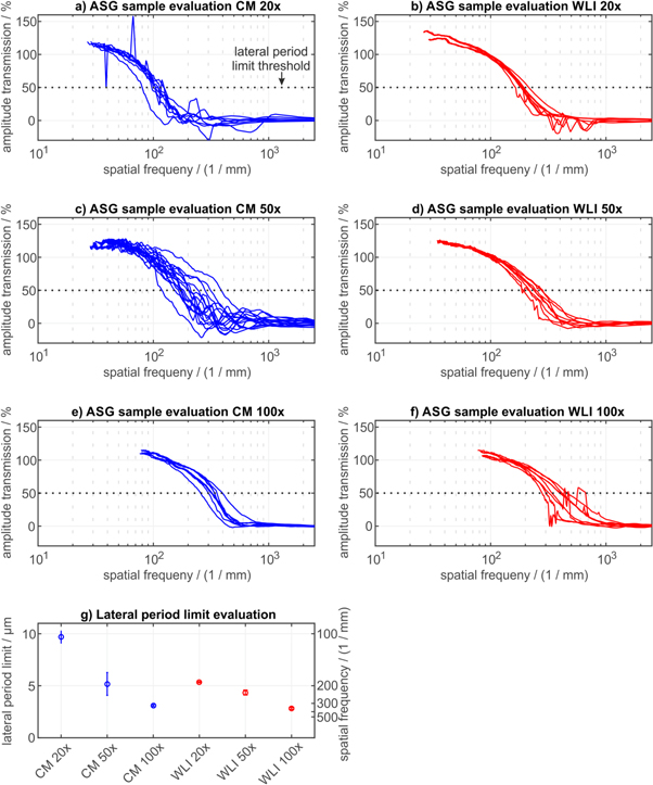
Figure 3. Results of the measurements of the ASG sample—determined transfer functions of the areal instruments CM and WLI (a)–(f) and resulting lateral period limit determination (g).
Download figure:
Standard image High-resolution image3.2. CIN-DLW material measure
The chirped standard that was manufactured by DLW was also only measured and evaluated for the areal surface topography measuring instruments. The pre-processing of the topography dataset by applying an F-operator for alignment was identical to the previously described evaluation of the ASG material measure. After this, a central profile of the 3D-topography was used to apply the small scale fidelity evaluation (see [22]). An example for this evaluation is shown in figure 4. Multiple sinusodial waves are fitted into the measured dataset and the amplitudes and wavelengths of the individual fits are calculated. The transfer function of the instrument can be calculated when all transferred amplitudes were divided by the nominal amplitude in order to obtain the transfer characteristics for varying spatial frequencies. As the chirped standard features a limited number of sinusoidal waves, there is a finite number of spatial test frequencies for this kind of transfer function determination. For example, the PTB chirped standard features 24 wavelengths ranging from 91 μm to 10 μm [6]. Additionally to the transfer function, for each measurement the small scale fidelity limit was determined which is defined as the shortest wavelength which is transferred within a certain threshold value for the deviation of the amplitude transmission. In the example of figure 4, the nominal amplitude of the chirped standard equals 400 nm. When a maximum amplitude deviation of ±25% is applied, the smallest wavelength which features a fitted amplitude between 300 nm and 500 nm is considered as the small scale fidelity limit. In the given example, the small scale fidelity limit equals 29.87 μm.

Figure 4. Example for a small-scale-fidelity evaluation [31]. Measured topography of a confocal microscope and fitted sinusoidal functions. Determination of the small scale fidelity limit.
Download figure:
Standard image High-resolution imageFor the specific evaluation the threshold for the small scale fidelity limit was chosen to ±50% of the original amplitude in order to ensure the best possible comparability to the results of the type ASG sample. Also, the amplitude transmission for all fitted wavelengths was calculated in order to characterize the transfer functions of the various measuring instruments and measuring configurations. The results of all chirp evaluations are shown in figure 5. There, the resulting points of the sinusoidal fits are shown for the CM and WLI measuring instruments for the varying magnification values 20×, 50× and 100×. The amplitudes of the different sinusodial fits from multiple measurements are summarized for each optical configuration. When the separate points of the various transfer functions are interpreted, the following conclusions can be drawn: just as with the results from the type ASG measurements, the transfer capabilities improve with higher magnification and the entire transfer function is shifted towards higher frequencies. Also the scattering of the transferred amplitudes is reduced with increasing magnifications—leading to more reproducible results. For the CM 50× measurements however, the determination of suitable illumination parameters was challenging due to optical artefacts that occur in regions with high frequencies when the illumination is set too large or too small. Four measurements for every setup were evaluated.
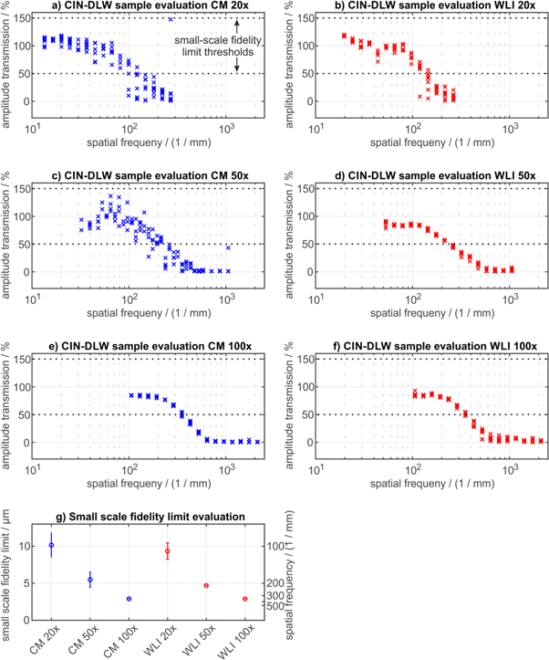
Figure 5. Results of the measurement of the CIN-DLW sample—determined transfer functions of the areal instruments CM and WLI (a)–(f) and resulting small scale fidelity limit (g).
Download figure:
Standard image High-resolution imageAdditionally, it should be noticed that with the CIN-DLW sample only a limited number of frequencies can be imaged within the samples that feature a lateral length between 100 μm and 800 μm. Thus, also the ultra-precision turned sample CIN-UPT was measured which represents a larger number of spatial frequencies and can additionally be measured with the profile measuring devices. The CIN-DLW material measure can fulfil its design purpose to determine reproducible transfer functions for areal surface topography measuring instruments.
3.3. CIN-UPT material measure
The evaluation of the CIN-UPT sample was performed identical as for the CIN-DLW sample in the previous section. For all confocal setups, profiles of two areal topography measurements were evaluated, otherwise four repetitions were performed and evaluated. The results of the transfer functions of the four different measuring instruments just as well as their determined small scale fidelity limit are summarized in figure 6. Similar results to the previous sample can be observed and similar small scale fidelity limit values in the micrometre-range were determined. However, for the areal instruments CM and WLI one phenomenon can be observed: because stitching is required to measure the entire set of different wavelength the results tend to scatter more significantly already for lower frequencies. The overall sample has a length of several millimetres. The results for the cut-off frequencies of the different measuring instruments which are again represented by the small scale fidelity limit are similar to the previously described sample CIN-DLW. For the two profile sensors SI and CCM, good results with small scale fidelity limits in the micrometre-range can be identified—these measuring systems are designed to acquire larger measuring lengths and no stitching is required. Thus, it can be concluded that the chirped sample which features larger structures is more suitable for the calibration of profile measuring instruments due to the required sampling length which is larger than for the CIN-DLW sample. The CIN-DLW samples are more suitable for areal measuring instruments because all frequencies can be imaged within a typical field of view.
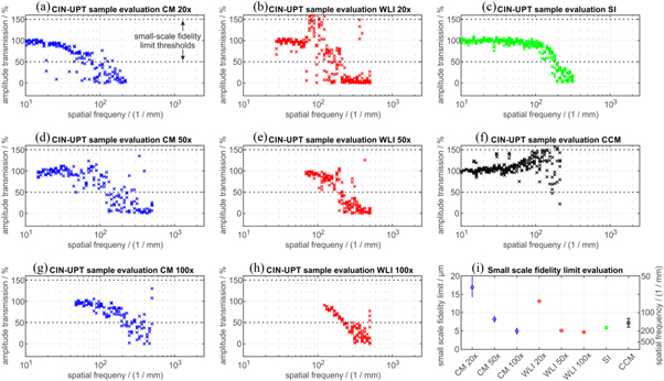
Figure 6. Results of the measurement of the CIN-UPT sample—determined transfer functions of the areal instruments CM, WLI, SI and CCM (a)–(h) and resulting small scale fidelity limit (i). Outliers that feature an amplitude transmission >160% are not displayed.
Download figure:
Standard image High-resolution image3.4. Rk-Standard—comparison to transfer behaviour based on time series modeling
The three previously described samples are specifically designed for the transfer function determination and it was shown that each of them has a specific field of application. In order to benchmark the results, they are compared with a different approach that was suggested by the authors and is based on time series modeling [23]. The approach is based on an autoregressive-moving-average (ARMA) model. When the time series ![$u\left[h\right],h=1,\,2,\,\mathrm{...},\,N$](https://content.cld.iop.org/journals/2051-672X/7/1/015024/revision2/stmpab0dc6ieqn3.gif) is considered as input signal, the output dataset z can be determined based on an ARMA model with the coefficients
is considered as input signal, the output dataset z can be determined based on an ARMA model with the coefficients ![$a[k]$](https://content.cld.iop.org/journals/2051-672X/7/1/015024/revision2/stmpab0dc6ieqn4.gif) and
and ![$b[l]$](https://content.cld.iop.org/journals/2051-672X/7/1/015024/revision2/stmpab0dc6ieqn5.gif) [32]:
[32]:
The mathematical term ![$\displaystyle {\sum }_{k=1}^{p}a[k]\cdot z[n-k]$](https://content.cld.iop.org/journals/2051-672X/7/1/015024/revision2/stmpab0dc6ieqn6.gif) describes the auto-regressive part with the degree p and
describes the auto-regressive part with the degree p and ![$\displaystyle {\sum }_{l=0}^{q}b[l]\cdot u\left[n-l\right]$](https://content.cld.iop.org/journals/2051-672X/7/1/015024/revision2/stmpab0dc6ieqn7.gif) the moving-average part with the degree q. When the corresponding model is interpreted in a way that the control dataset for the ultra-precision manufacturing of a certain deterministic rough surface is the input data u of the measuring instrument and the measured data represents the output data z of the model, the ARMA-coefficients describe the transfer behavior of the measuring instrument. Thus, when equation (3) is transformed into the frequency domain, and an algebraic fit of the model coefficients
the moving-average part with the degree q. When the corresponding model is interpreted in a way that the control dataset for the ultra-precision manufacturing of a certain deterministic rough surface is the input data u of the measuring instrument and the measured data represents the output data z of the model, the ARMA-coefficients describe the transfer behavior of the measuring instrument. Thus, when equation (3) is transformed into the frequency domain, and an algebraic fit of the model coefficients ![$a[k]$](https://content.cld.iop.org/journals/2051-672X/7/1/015024/revision2/stmpab0dc6ieqn8.gif) and
and ![$b[l]$](https://content.cld.iop.org/journals/2051-672X/7/1/015024/revision2/stmpab0dc6ieqn9.gif) is executed, the frequency-dependent transfer behavior of the measuring instrument can be determined based on its input and output data. This was investigated and proven for different surfaces (see [23]). In doing so, it was shown that the Rk-standard, whose nominal geometry for manufacturing is based on an actual component surface and known precisely, can lead to the most precise determination of the transfer function for different measuring instruments. The virtual manufacturing dataset is considered as the input and the measured data of a topography measuring instrument as the output of a time series. Thus, with the fit of a model for the transfer behaviour determination, additional information for comparison can be obtained based on this fourth sample.
is executed, the frequency-dependent transfer behavior of the measuring instrument can be determined based on its input and output data. This was investigated and proven for different surfaces (see [23]). In doing so, it was shown that the Rk-standard, whose nominal geometry for manufacturing is based on an actual component surface and known precisely, can lead to the most precise determination of the transfer function for different measuring instruments. The virtual manufacturing dataset is considered as the input and the measured data of a topography measuring instrument as the output of a time series. Thus, with the fit of a model for the transfer behaviour determination, additional information for comparison can be obtained based on this fourth sample.
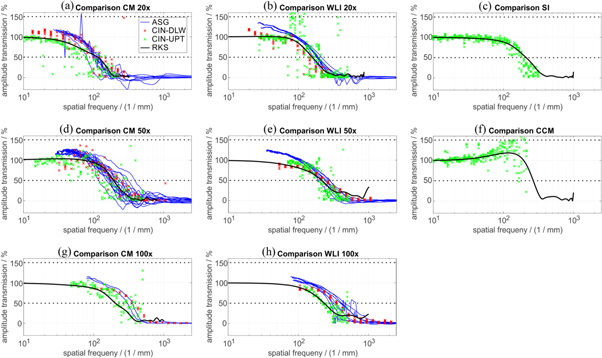
The Rk-standard was measured once with every areal topography measuring setup and four repetitions with the two profile measuring instruments were performed. Based on the obtained measured data, a time series model was determined based on only one profile per measuring configuration which provides a linear approximation of the instruments transfer behaviour. It is examined whether this approach is more universally applicable than the previously described samples. In doing so, the benchmark displayed in figure 7 was determined where all transfer functions that were determined with the numerous methods are displayed. This includes as well the transfer functions that were determined based on the fit of the ARMA-model.
Figure 7. Comparison of all obtained transfer functions based on the different methods ASG, CIN-DLW, CIN-UPT and RKS. Outliers that feature an amplitude transmission >160% are not displayed.
Download figure:
Standard image High-resolution image
It can be observed that the transfer functions based on the ARMA-approach do well agree with the other transfer functions and realistic results can be generated. The cut-off frequencies of the different approaches do agree well for all instrument setups. Only for high frequencies the approach based on the ARMA-model leads to deviations if the sampling theorem is violated. Thus, the transfer functions were calculated to a maximum frequency of  Generally, it can be shown that the approach of time series modeling with the Rk-Standard is a universally applicable method for the transfer function determination of different profile and areal surface topography measuring instruments. However, one limitation of the model should be considered: as a linear model, the time series model cannot image some physical effects that have non-linear characteristics.
One particular example for physical effects that can be imaged with the ARMA-model can however be observed for the CCM measurement. It can be assumed that curvature depending effects at large spatial frequencies lead to an increase of the amplitude transmission when the CIN-UPT sample is measured. Mauch et al described this effect [33]. This effect would be also expected for the confocal microscope but can only be observed for the CCM measurement. This effect can also be imaged with the transfer function of the ARMA-model. However, all measuring instruments feature non-linear effects that cannot be considered by the model. As the agreement between the measured transfer functions and the transfer functions of the ARMA-model is high, it can be concluded that these effects do not have a major influence on the transfer behaviour.
4. Conclusion
For the determination of the lateral resolution limit, there are the two approaches of the star-shaped grooves material measure and the chirped standard described in the current ISO standardization. The described study carried out a comprehensive comparison of these two methods and benchmarked them against another method for transfer function determination which is based on time series modeling.
Four different instruments were applied for measurements and their results of the different samples were evaluated and compared. Those measuring instruments that could measure all samples could also achieve comparable results for both material measures. Besides this, the following advantages and disadvantages of the two methods could be determined:
The star-shaped grooves sample (ASG) provides stepless frequencies and allows a measurement of these frequencies without any stitching in one field of view. Also large spatial frequencies can be imaged with the sample. However, the sample is only applicable for areal instruments and the rectangular test structures are not compliant to a realistic measuring task. Additionally, due to the fact that the evaluation is based on two extracted profiles, every test frequency is only represented by one pair of points in each profile, leading to a large impact of single outliers on the measurement result. This is visible in the results, where also negative values for the amplitude transmission occur due to the described evaluation method. The evaluation also considers only deviations in the amplitude transmission in one direction as a threshold value of 50% amplitude transmission is applied for the lateral period limit determination.
The chirped standard in contrast works for both profile and areal measuring principles and provides more realistic test structures. Due to the different requirements, it was observed that some chirped standards are more suitable for areal and some for profile measuring instruments. Because one point in the transfer function is determined by an entire sinusodial wave the approach is more robust when single outliers in the dataset are present as the fitted amplitude is relevant to determine the amplitude transmission. The disadvantages are that only discrete frequency values are provided by the sample and no stepless calibration is possible. Additionally, due to the high contrast of the surface and the steep angles, the illumination properties of the applied microscope are more challenging to determine than for the ASG sample. In order to image enough frequencies also stitching can be required which introduces additional deviations. Thus, it is recommended to apply the ASG sample when only the lateral period limit is of interest. When however, the entire transfer function should be determined, the chirped standard is suitable both for profile and areal surface topography measuring instruments and can provide reproducible results. The small scale fidelity limit also considers deviations in the amplitude transmission both in the positive and negative direction.
When all results were compared to transfer functions determined by a time series model approach that uses measurement data of the Rk-standard, a high agreement could be achieved. Thus, this approach was proven to be universally applicable for various measuring instruments. However, some non-linear effects that occur during the measurement are not considered by the linear ARMA-model.
The described methods can be applied to calibrate surface topography measuring instruments for arbitrary applications. For every precision measurement it needs to be ensured that the transfer characteristics of the applied instrument match the requirements. It was shown that different measuring principles can be characterized with the material measures for the determination of transfer characteristics. In future work, the time series model approach will be further examined.
Acknowledgments
This research is funded by the Deutsche Forschungsgemeinschaft (DFG, German Research Foundation)—252408385—IRTG 2057. We thank AMETEK Germany GmbH (BU Zygo) for the possibility to obtain measurements at their laboratory.