

Abstract
In this paper, we will review the development and use of an ISO standardised framework to allow calibration of surface topography measuring instruments. We will draw on previous work to present the state of the art in the field in terms of employed methods for calibration and uncertainty estimation based on a fixed set of metrological characteristics. The resulting standards will define the metrological characteristics and present default methods and material measures for their determination—the paper will summarise this work and point out areas where there is still some work to do. An example uncertainty estimation is given for an optical topography measuring instrument, where the effect of topography fidelity is considered.
Export citation and abstract BibTeX RIS

Original content from this work may be used under the terms of the Creative Commons Attribution 4.0 license. Any further distribution of this work must maintain attribution to the author(s) and the title of the work, journal citation and DOI.
1. Introduction
In 2018, the first international specification standard was published that goes some way towards establishing a framework for calibration of areal surface topography measuring instruments, including those employing optical techniques [1]. The work that led up to the development of the ISO 25178 part 600 is summarised elsewhere [2–5]; this review will present what has been achieved since and discuss some remaining research.
The optics and semiconductor manufacturing industries have well-established calibration infrastructures for optical measurements of surface topography, albeit for very specific surface types [6–8]. However, these infrastructures are less well developed for many precision manufacturing industries that rely on machining of complex surface geometries [9–11]. The highly complex freeform geometries and textures as found, for example, in the automotive, aerospace and medical parts industries, mean that many of the established calibration techniques for optical surface measurements may not be directly relevant. In addition, with the industrial uptake of additive manufacturing techniques, the complexity of the resulting surfaces is leading to new measurement challenges [12–14].
When manufacturing surfaces with complex topography, industrial instrument users rely on well-established techniques to demonstrate that a process is under control and that the response of an instrument is not changing significantly with time. Examples found in common practice include statistical process control, gauge R&R studies and measurement system analysis. Whilst these approaches are mature and clearly allow manufacturing to continue and advance, they do not lead to a culture of uncertainty estimation in manufacturing and, hence, tolerancing of complex surfaces is difficult and geometrical product specification principles cannot always be applied.
Looking from a different perspective, it is commonplace in many manufacturing industries to hear users expressing alarm about the incompatibility of optical instruments with contact methods of measuring surface topography, and these concerns are often borne out in formal comparisons (for example, [15–17]). In many cases, the difference between the results from optical and contact instruments can be explained after critical assessment of the measurement conditions and sample geometries [18–20], but there is still an undercurrent of concern in some industries. One of the reasons for differences between the results from optical and contact instruments with complex surfaces is the lack of a calibration framework for optical instruments. The crux of the issue is that, while it is relatively simple to understand and model the physical interaction of a contact probe tip with a surface (see, for example, [21–23]), it is not so simple to model the equivalent optical interaction [24, 25]. The complexity of optical instrument measurement models (see, [20, 26–28], for recent research to establish optical instrument models), especially with complex surfaces, means that a first-principles uncertainty budget calculation based on establishing an appropriately accurate measurement model is a highly complex task (if possible at all in some cases) and, to the authors' knowledge, has only been realised in the optical manufacturing sector (for example, see [29–35]).
The ISO framework being developed attempts to simplify the calibration process by introducing a number of common or instrument-independent metrological characteristics—parameters that can be determined with a suitable material measure (or in some cases, the object being measured) and procedure; and the resulting parameter values (after suitable scaling to account for their statistical distribution) can then be propagated through a measurement model to give an estimate of measurement uncertainty. The framework only applies if certain well-defined assumptions about the measurement scenario are adhered to, but it is a solid start and will hopefully enhance the kudos of optical instruments in the manufacturing industry. In section 2, we will summarise the framework, building on the previous publications [2, 4, 36], in section 3, we will present the recent development of material measures and in section 4, we will give an example uncertainty estimation using the metrological characteristics framework. It is highly recommended that these previous publications [2, 4] are consulted prior to reading this review.
2. The ISO metrological characteristics framework
The metrological characteristics that have now been published in ISO 25178 part 600 [1], are presented in table 1. Note that, since the publication of Leach and Giusca [2, 3, 36], the metrological characteristic of perpendicularity has been renamed x-y mapping deviation. Also, while topography fidelity was not covered in Leach and Giusca [2], there is a short overview of the characteristic in Leach et al [3], and it is covered in detail in section 2.7.
Table 1. List of metrological characteristics in 1.
| Main potential | ||
|---|---|---|
| Metrological characteristic | Symbol | error along |
| Amplification coefficient | αx , αy , αz | x, y, z |
| Linearity deviation | lx, ly, lz | x, y, z |
| Flatness deviation | zFLT | Z |
| Measurement noise | NM | Z |
| Topographic spatial resolution | WR | Z |
| x-y mapping deviations | Δx (x, y), Δy (x, y) | x, y |
| Topography fidelity | TFi | x, y, z |
The definition of metrological characteristic as it is written in ISO 25178 part 600 is given below.
Metrological characteristic: <measuring equipment> Characteristic of measuring equipment, which can influence the results of measurement.
Note 1 to entry: Calibration of metrological characteristics is often necessary.
Note 2 to entry: The metrological characteristics have an immediate contribution to measurement uncertainty.
In other fields (for example, coordinate metrology), the term metrological characteristic is used for any characteristic that affects a measurement result and its uncertainty. However, one of the central themes of ISO 25178 part 600, is that the definition should only be applied to the characteristics listed in table 1. These metrological characteristics are designed to capture all of the factors that can influence a measurement result (often called influence quantities or influence factors) and, after their probability density function and resulting statistical values are established, can be propagated appropriately through a specific measurement model to estimate measurement uncertainty. The ISO 25178 series also includes the so-called parts 60X [3] which are specific to a number of common instrument types and define instrument terms and some basic theory of operation. However, the 60X parts also list influence quantities (note that current drafts for updates to the parts 60X move the influence quantities from the normative to the informative sections but, at the time of writing, this move has not been agreed by ISO Technical Committee 213). These influence quantities are only given to show how they affect the metrological characteristics—it is not expected that they would be used to estimate uncertainty. Estimating measurement uncertainty for a surface topography measurement (and a texture parameter calculation using the measured data) is highly complex (see examples in Haitjema [36–40]) and the metrological characteristics have been explicitly defined so as to make this process simpler to apply in industry. A number of example uncertainty budgets using metrological characteristics have been published [4, 36, 41–44] but the publication of more examples is required to build up the database and promote industrial adoption. The distinction between influence quantities and metrological characteristics are made in figure 1. The metrological characteristics framework provides an approximation of the measurement uncertainty (albeit, it will always overestimate), as it may use some influence quantities more than once, but it is designed to be feasible to employ in industry and to improve the comparability of results from different instruments.
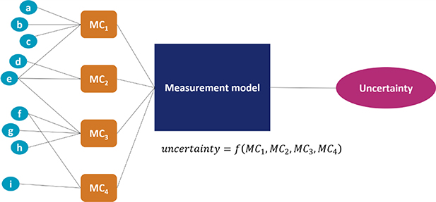
Figure 1. Illustration of the metrological characteristics framework to estimate measurement uncertainty. a to i are influence quantities and MC1 to MC4 are metrological characteristics.
Download figure:
Standard image High-resolution imageNote that there is an important distinction between two types of metrological characteristics that is not made explicitly clear in the ISO 25178 documents, particularly that some metrological characteristics can be determined irrespective of the surface type. These are amplification coefficient, linearity deviation (see section 2.2), flatness deviation (see section 2.3), x-y mapping (see section 2.5) and topographic spatial resolution (see section 2.6). These metrological characteristics are properties of the instrument and its environment and can be determined and used in an uncertainty estimation independent of the measured topography. On the contrary, some metrological characteristics are dependent on the surface being measured. These characteristics are measurement noise (see section 2.4) and topography fidelity (see section 2.7). To quantify these object-dependent metrological characteristics requires the surface topographic properties to be understood or procedures to be put in place that capture enough information about the surface to allow its effect on the measurement to be taken into account. These issues are discussed in the relevant sections in this paper, but how they should be quantified and used in uncertainty estimation are still open research questions [25].
Whilst ISO 25178 part 600 lists and defines the metrological characteristics, ISO 25178 part 700 will describe default procedures and material measures to determine them. It is expected that part 700 will be published in late 2020 or early 2021. It is not the purpose of this review to repeat all the material in the standards—many of the default procedures are based on those described in Leach and Giusca [2], but some recent additions are presented. There are also published good practice guides on determination of the metrological characteristics for stylus instruments [41], interferometric microscopes [42] and imaging confocal microscopes [43]. Furthermore, there are publications on the determination of the metrological characteristics for focus variation microscopes [45, 46], point autofocus instruments [47, 48] and confocal microscopes [49].
2.1. Amplification coefficient and linearity deviation
The following definitions are from ISO 25178 part 600 and their general use is described elsewhere [3, 4, 50, 51].
Amplification coefficient: Slope of the linear regression line obtained from the response function
Linearity deviation: Maximum local difference between the line from which the amplification coefficient is derived and the response function
An example of the determination of the amplification coefficient and the linearity deviation is given in figure 2. Note that the amplification coefficient is characterised by a single number; its deviation from unity, and its uncertainty, are input quantities for an uncertainty evaluation. The linearity deviation is given as a function of the z-axis coordinate. The default method to determine both the amplification coefficient and linearity deviation in the axial direction (z-axis) that will be described in ISO 25178 part 700 is to use a series of step height material measures (see [3, 4]). However, there have been a number of recent advances that are described below (there are also several older, but still relevant, examples of step height measurement uncertainty estimation, for example [52–55]).
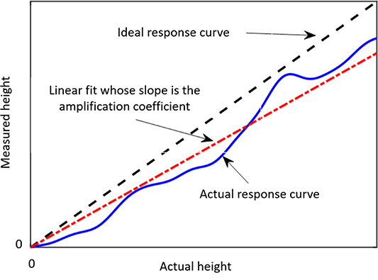
Figure 2. Illustration of the derivation of the amplification coefficient and linearity deviation.
Download figure:
Standard image High-resolution imageA relatively simple procedure to determine the amplification coefficient and linearity deviation for long z-axis range instruments has been recently reported and will likely be included in ISO 25178 part 700 [56]. The procedure employs a material measure containing a number of step heights (positive or negative) and stitches together segments of the response function. For each segment, the heights on the artefact are measured and compared against the calibration values. Since the steps have one common reference plane, they can be regarded as belonging to a common scale and used to build up the segments of the response function. Measurements of as many segments as necessary to cover the z-axis range can be performed without the need for accurate positioning; for example, a series of thin blocks could be used.
Referring to figure 3, for each segment of the response function, an interpolating function is fitted to the discrete set of pairs of height values, for example, a parabola. The following is an example for negative (grooved) steps but can be easily converted to positive steps. The absolute position of the reference point remains unknown and is set equal to the measured value. The pairs of depth values of the highest position are used for the first segment. An interpolating function for the first segment, which uses the calibration values as the dependent variables and the measured (indicated) values as the independent variables, is used to determine the actual position of the next segment. This function is related to a segment of the inverse response function. Using the interpolation function of the first position, the actual position of the next segment's starting point is the function value of the measured position of the reference plane of the second position. Interpolating the pairs of height values of the second position, the third position's starting point can be obtained, and so on until the axial range is covered.

Figure 3. Construction of a response curve by stitching curve segments determined by measurements on a material measure with grooves representing a set of differing height values on one artefact with one common reference plane. The abscissa represents the indicated values of the instrument (zi ) and the ordinate the calibrated values (za ) (from [56]).
Download figure:
Standard image High-resolution imageMeasuring a tilted flat is an efficient and appropriate method to asses z-axis linearity deviation. The obvious advantage of using a tilted flat is that the linearity curve from the lowest to the highest measured point is measured continuously instead of being interpolated from the limited number of discrete points on the calibration curve that are assessed using discrete steps. Assuming a negligible flatness deviation of the flat surface used, zero instrument flatness deviation and ideal linearity of the instrument in the x-y direction, the profile deviations from a fitted flat plane can be taken directly as the linearity deviation (see also [57]). The flatness deviations can be eliminated to a major extent by measuring the flat surface in the levelled position and taking the difference with the tilted position. This method's usefulness for this purpose was already described in ISO 12179 [58], and in a reference specimen design [59]. Because of the rotation, amplification and x- and y-linearity deviations may still have some influence; a detailed treatment of this is given elsewhere [60]. A further reduction—and a simplification of the calculations—can be achieved by a reversal method: the flat measured at two tilt positions—one over the desired angle (dependent on the z-axis range that is being assessed), measurement A, and one where the flat is tilted over exactly the opposite angle, measurement B. The difference between these two measurements, (A–B), gives the linearity deviation, where the flatness deviations of both the flat specimen and the instrument are eliminated. A further reduction is possible by taking the difference (B–A), rotating this result 180° (around the z-axis) and averaging this result with the (A–B) result. Figure 4 illustrates this procedure. A final result is obtained by averaging over the y-coordinates.

Figure 4. Illustration of the reversal method for determining the linearity deviation lz. A is the measurement result of a tilted optical flat; B is the result of the measurement where the flat is tilted opposite to the tilt in A. The difference (A–B) gives a basis for the linearity deviation, where the difference (B–A), denoted by (B–A)' as it is rotated 180° around the z-axis, gives another independent linearity deviation estimation. The final linearity deviation is calculated by averaging the calculated flats over all y-coordinates and removing a least-squares line. As both determinations (A–B) and (B–A) give twice the linearity, the sum must be divided by four. This gives the linearity deviation as indicated in the lower graph, resulting in 0.2 µm linearity deviation over 80 µm height difference, measured in some 1000 small steps.
Download figure:
Standard image High-resolution imageFor optical measurement of relatively large step height artefacts or those with narrow grooves, the lateral and axial responses may be coupled in regions near groove edges. This coupling effect, mainly caused by beam shadowing, results in an accuracy loss or incorrect result. The limited energy loss (LEL) method has been proposed to model the coupling effect at the edge of a groove and clearly demonstrates the measurement areas for height evaluation [61]. The LEL method determines the most effective measurement areas for height evaluation using the theoretical relationship between groove geometry and the optical instrument parameters. The LEL method suggests changes to the measurement procedure outlined for step height analysis in ISO 5436 part 1 [62], and proposed in ISO 25178 part 700. The LEL criteria is briefly mentioned in part 700 and included in the Chinese national specification standard [63].
The default method to determine both the amplification coefficient and linearity deviation in the lateral directions (x- and y-axes) that will be described in ISO 27178 part 700 is to use grid type material measures (see [3, 4]).
2.2. Flatness deviation
The following definition is from ISO 25178 part 600 and its general use is described elsewhere [3, 4].
Flatness deviation: Deviation of the measured topography from an ideal plane
In this definition, the flatness deviation is understood as the flatness deviation of the instrument's flatness reference; it is the flatness deviation that the instrument would output if a perfectly flat specimen were measured. The default method to determine flatness deviation that will be described in ISO 27178 part 700 is to use an optical flat material measure (see [3, 4, 106]). The effect of the optical flat itself and the effect of the instrument noise (see section 2.4) can be reduced by measuring different areas on the optical flat and averaging the topography values [64]. This averaging procedure principally reduces all flatness components of the optical flat except for the sphericity, cylindricity and torque: if both the instrument and the optical flat have one of these form deviations, they will not be reduced by averaging. However, these effects will be small in practice. Rotating the optical flat 90° for half of the measurements will reduce the effect of joint torque and some cylindricity.
2.3. Measurement noise
The following definitions are from ISO 25178 part 600 and their general use is described elsewhere [3, 4].
Instrument noise: Internal noise added to the output signal caused by the instrument if ideally placed in a noise-free environment.
Measurement noise: Noise added to the output signal occurring during the normal use of the instrument.
The instrument noise is only used for specification purposes—it will be the best achievable noise value and the default material measure is an optical flat. Clearly, this value should not be used when estimating measurement uncertainty (unless the measurand is a flat surface under ideal conditions). For this, the measurement noise should be used. Instrument noise refers to the internal noise added to the output signal caused by the instrument if ideally placed in a noise-free environment, whereas measurement noise refers more generally to noise added to the output signal occurring during the normal use of the instrument. The instrument noise is, therefore, approximated by the minimum achievable measurement noise under the most ideal circumstances.
There is no default material measure for measurement noise, as it will vary significantly with different surface topography types (see [20, 65]). As such, measurement noise should be determined using the surface being measured, or at least, a surface that is representative of the type of surfaces being measured.
In order to be reproducible and comparable to other results, the measurement (and instrument) noise values should be stated with the relevant data acquisition time, the number of independent data points and any default filtering of the surface topography [66].
In general, noise will make subsequent measurements vary, depending on the surface topography and the surface parameter considered. Also, noise may cause a systematic deviation for certain parameters. For example, amplitude parameters, such as Sa, Sq and Sz, will in general show an increase when more noise is present, which is not revealed by repeated measurements. This effect is known as 'noise bias' and has been described by several authors [64, 67, 68]. Noise bias limits the usefulness of 'rms noise repeatability' as a measure for measurement noise [69].
2.4. X-y mapping deviation
The following definition is from ISO 25178 part 600 and its general use is described elsewhere [3, 4].
X-y mapping deviation: Gridded image of x- and y-deviations of actual coordinate positions on a surface from their nominal positions
The default method to determine the x-y mapping deviation that will be described in ISO 27178 part 700 is to use grid type material measures (see [3, 4]).
2.5. Topographic spatial resolution
The following definition is from ISO 25178 part 600 and its general use is described elsewhere [3, 4, 70].
Topographic spatial resolution: <surface topography> Metrological characteristic describing the ability of a surface topography measuring instrument to distinguish closely spaced surface features.
The choice of criterion to quantify the topographic spatial resolution is left to the user, as it will be dependent on the instrument and surface types, and especially the measurement model. The examples listed in ISO 25178 part 600 are given below.
- lateral period limit—spatial period of a sinusoidal profile at which the height response of the instrument transfer function falls to 50% [71, 72];
- stylus tip radius [73];
- lateral resolution—smallest distance between two features which can be recognised;
- width limit for full height transmission—width of the narrowest rectangular groove whose step height is measured within a given tolerance;
- small scale fidelity limit (see section 2.7);
- Rayleigh criterion—quantity characterising the optical lateral resolution given by the separation of two point sources at which the first diffraction minimum of the intensity image of one point source coincides with the maximum of the other;
- Sparrow criterion—quantity characterising the optical lateral resolution given by the separation of two point sources at which the second derivative of the intensity distribution vanishes between the two imaged points; and
- Abbe resolution limit—quantity characterising the optical lateral resolution given by the smallest diffraction grating pitch that can be detected by the optical system.
The first edition of ISO 25178 part 700 will not contain default material measures for topographic spatial resolution—the subject matter is not considered mature enough to standardise yet and the type of material measure will be dependent on the criterion used [106]. Periodic, chirped [74, 75] and star-shaped material measures are given as example material measures. There has been a recent paper analysing the stability of various methods to determine the lateral period limit using star-shaped material measures [76].
An example calibration for topographic spatial resolution is the determination of the instrument transfer function (ITF), from which several of the parameters in the list above can be determined. The ITF is defined as the square root of the ratio of the measured power spectral density of a surface structure to its known or independently determined power spectral density. In essence, the ITF quantifies the response of a topography-measuring instrument to specific spatial frequencies in the surface geometry (figure 5, [70]). The ITF is widely used in the testing of optical components, such as lenses and mirrors, and can be calibrated using a variety of available artefacts, including small step features etched into glass. However, it is understood that the range of applicability of the ITF is limited, particularly for surfaces with rough or complex textures or high slope angles. It is also not clear how an ITF evaluation can be incorporated into an uncertainty budget. Consequently, although the ITF concept is defined in the draft ISO 25178 part 700 document, methods of ITF calibration remain informative rather than normative [106].
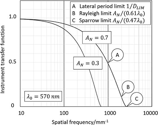
Figure 5. Instrument transfer function of a coherence scanning interferometer instrument in terms of spatial frequency for incoherent illumination at a wavelength λ0 = 570 nm. This is a theoretical result for the effects of optical filtering only, in the limit of small surface height variations, courtesy of Prof. Peter de Groot (ZYGO).
Download figure:
Standard image High-resolution imageISO 25187 part 600 suggests that the methods outlined in VDI/VDE 2655 part 1.3 [77], can be used to determine topographic spatial resolution. VDI/VDE 2655 part 1.3 recommends the use of material measures with multiple gratings, with multiple periods; each with rectangular cross-section and having the same amplitude (these are commercially available). Such a material measure does not need to be calibrated as a low spatial frequency part of the grating (i.e. one where the amplitude transmission is assumed to be 100%) can be used as the reference. However, the response to a rectangular structure with a certain size does not necessarily predict the response to other sizes or shapes, so care should be taken when using rectangular cross-section topographies with optical instruments, especially when approaching an instrument's linear operating range (see section 2.7 and [27, 78, 79]).
Topographic spatial resolution in the z-axis is not defined in ISO 25178 part 600 or the draft of part 700 (but see [80]).
2.6. Topography fidelity
The metrological characteristic topography fidelity has been introduced into the ISO 25178 calibration framework as a kind of miscellaneous category for all contributions to the uncertainty budget—including a broad range of surface-dependent errors—that are not captured by the more well-known calibrations described in sections 2.2–2.6 (see [25], for a discussion on the current status). Common issues that are reported include outliers, missing points and other unexpected topographic features (see, for example, [17, 81–83]); whilst these effects may be clear when measuring a simple topography, they may not be evident at all for a complex topography, although a well-designed material measure for topography fidelity should highlight and, hopefully, quantify these issues. The following definitions are from ISO 25178 part 600.
Topography fidelity: <line profiling> <areal topography> Closeness of agreement between a measured surface profile or measured topography and one whose uncertainties are insignificant by comparison.
Small scale fidelity limit: Smallest lateral surface feature for which the reported topography parameters deviate from accepted values by less than specified amounts.
Proposed methods for calibrating topography fidelity are sparse but a common theme is to use a material measure having a shape that is close to the measurand, and that has been calibrated independently and/or or manufactured in such a way that the real geometry is known. Measuring this artefact using the instrument to be evaluated may give quantitative information about the deviations that can be used in an uncertainty budget (see example in section 4).
Artefacts are under development that include a multitude of established difficult-to-measure features such as steep steps and grooves of various spacings and depths. Example artefacts under development include chirp artefacts [74, 75] that are comprised of sinusoidal waves of varying wavelengths and amplitudes, and an artefact (in fact a collection of artefacts on a single substrate) ([84], section 3) that contains a multitude of surface structures within a limited area. Recently, circular chirped artefacts with several lateral sizes have been developed [85, 86]. Figure 6 shows a coherence scanning interferometry (CSI) measurement of the circular chirped artefact—the features that can be seen in the measured data above the nominal height of the square wave features are exactly those that the topography fidelity metrological characteristic is designed to represent. Although there have been proposals for metrics or measures of agreement to allow for reporting and specifying of topography fidelity [87], nothing is agreed at the time of writing. How to use the data from figure 6 in an uncertainty budget for a different topography remains an open question, although it would be highly relevant data for gauge R&R studies or measurement system analysis.
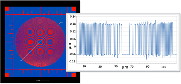
Figure 6. CSI measurement of the PTB circular chirped artefact [85]. Left: Plan view of the artefact showing the extracted profile trajectory. Right: Profile of the artefact. Both figures courtesy of Dr Martin Fay (ZYGO).
Download figure:
Standard image High-resolution imageIt seems, however, unrealistic to suppose that a single artefact can be designed to determine topography fidelity that includes all possible surface structures. For less defined structures than the reference specimen, estimates of the uncertainties are not sufficiently reliable. A further issue is that many of these proposed structures have sharp edges or other features that result in measurement outliers, missing data, false data or, with interferometry, fringe-order errors that are not easily summarised as statistical variations for the purpose of an uncertainty budget. Finally, for many of these proposed material measures, not much more can be done than to take deviations for granted and to try to quantify these without a solid understanding as to the origins of the errors (see example in section 4). Clearly, there needs to be more research to try to find appropriate methods and material measures for determining topography fidelity, and especially on how to apply the concept in uncertainty budgets [25].
The small scale fidelity limit is related to topographic resolution, but includes effects that are not captured by conventional transfer function approaches to resolution. Notes to the definition in ISO 25178 part 600 state that the limit can be positive or negative, that a practical maximum deviation could be 10% (this value is of course arbitrary and case dependent) and that it depends on the type of topography being measured. In VDI/VDE 2655 part 1.3, it is suggested that chirp artefacts should be used to determine the small scale fidelity limit [75, 84–86], but it is not clear how the resulting measurement value could be used in an uncertainty budget.
3. Material measures
The default material measures used to determine the metrological characteristics will feature in ISO 25178 part 700 [106] and were reviewed in Leach et al [3], updated in Carmignato et al [88], and their specifications are given in ISO 25178 part 70 [89]. Note the use of the term 'default' material measures—the standard does not mandate the use of these material measures—the user is free to use any appropriate material measure, but they must state what has been used. Defaults are what is assumed if details are not included with a particular measurement outcome, although it is good practice to always include all relevant details, whether default or not. Alternative calibration techniques with clear traceability paths are equally acceptable, depending on the capabilities of the instrumentation. Example techniques include those based on an independent realisation of the metre using a natural emission wavelength, the value for which has been established with a known uncertainty [90, 91].
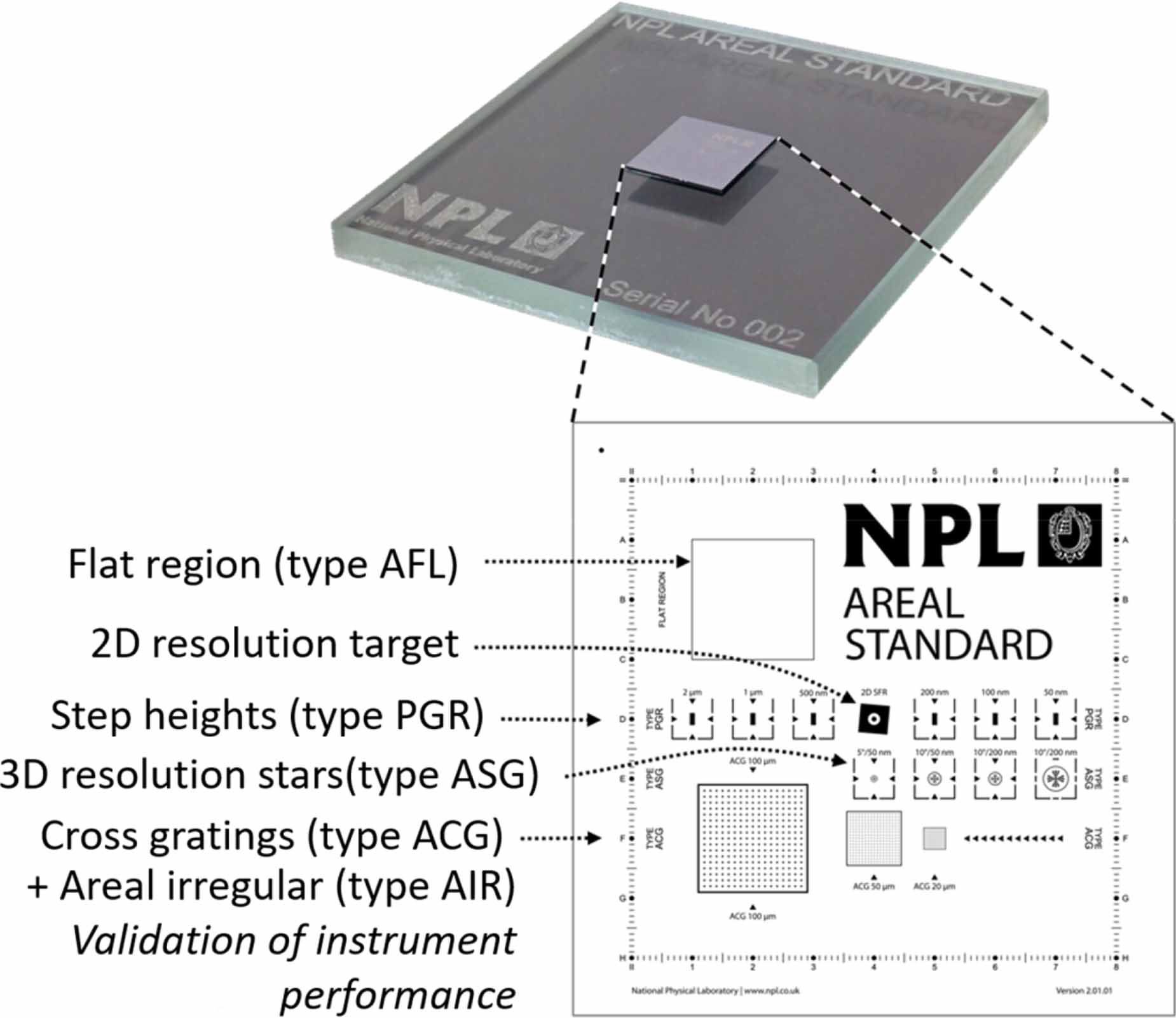
The National Physical Laboratory (NPL) ([92], figure 7) and the University of Kaiserslautern ([57, 84], figure 8) have both developed single-substrate artefacts that include all the measures required to determine the metrological characteristics (with the exception of topography fidelity in the NPL artefact).

Figure 7. The NPL Areal Standard for areal topography measuring instruments, featuring a range of areal material measures intended to enable application of ISO 25178 part 700. The (10 mm)2 multifunction silicon artefact is shown mounted on a precision glass substrate. ©National Physical Laboratory, used with permission [92].
Download figure:
Standard image High-resolution image
Figure 8. The Universal Calibration Artefact from University of Kaiserslautern, courtesy of Dr Matthias Eifler (University of Kaiserslautern, from [84]).
Download figure:
Standard image High-resolution image4. Example with CSI
As already discussed, model functions differ in complexity from one measurement application to another. Examples of uncertainty estimations using metrological characteristics are given elsewhere [4, 36, 41–44], but these examples do not include the topography fidelity contribution. In the example given here, a simple procedure to estimate the contribution of areal topography fidelity is included, based on recommendations in VDI/VDE 2655 part 1.3 [77].
The combined standard measurement uncertainty is calculated as a combination of type A and type B standard measurement uncertainty components. It is assumed that the reader is familiar with conventional methods for uncertainty estimation based on the Guide to Expression of Uncertainty in Measurement [93, 94]. Specific to uncertainty estimations according to the GUM are the sensitivity coefficients associated with each relevant metrological characteristic, which are derived from the model function and hence, affected by the way the measurement is performed.
In the example, a CSI was used as the instrument under test [95, 96]. Following the measurement of a sinusoidal material measure (a nickel artefact with nominal wavelength of 100 µm and nominal amplitude of 1.5 µm, shown in figure 9), the uncertainty associated with the calculation of the Sq parameter (root mean square height of the scale limited surface), is used as an example. The CSI measurements were performed with a 5.5 × magnification objective at 1 × zoom setting (with a numerical aperture of 0.15, a field of view of 1.6 mm × 1.6 mm and a sample spacing of 1.47 µm), and the data were levelled by least-squares plane removal, a Gaussian convolution S-filter with a nesting index of 2.5 µm was applied and an area of 0.8 mm × 0.8 mm (544 × 544 pixels) was extracted to give an S-F surface using the default values from ISO 25178 part 3 [72].
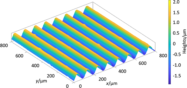
Figure 9. Example CSI measurement of the sinusoidal material measure.
Download figure:
Standard image High-resolution imageA method of uncertainty estimation that can be applied to any parameter was given by Haitjema [36], and involves a re-calculation of the full topography while varying the metrological characteristics and considering the variation in the calculated parameters. As access to all raw measurement data, manipulation of this data and access to filtering and parameter algorithms are rarely feasible for most users, an example is given for the Sq parameter that is well defined and for which some effects can be calculated without the need for knowing the topography.
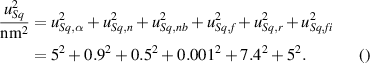
The analysis is restricted to the most relevant metrological characteristics for which the uncertainty can be estimated. For example, the non-linearity in z (lz) and the amplifications and non-linearities in x and y (αx, αy, lx and ly ) are expected to have no significant effect on the Sq parameter. Following the good practice guidelines outlined elsewhere [42], the total standard measurement uncertainty is given by

where  is the contribution to the uncertainty of Sq due to the amplification coefficient,
  is the contribution due to measurement noise,
  is the contribution due to the systematic bias on the Sq value due to noise,
  is the contribution due to the flatness deviation,
  is the contribution due to the limited topographic spatial resolution and
  is that due to topography fidelity.
Note that the Sq parameter, assuming all z-axis coordinates are given as S-F surface topography coordinates, is given by
and the equation for propagation of uncertainty is given by [97]
where N is the number of measured height values,  are the measured height coordinates and
  is the uncertainty in the height coordinates due to the metrological characteristic p, as given in equation (1). The various components in equation (1) will now be discussed in detail.
The z-axis scale for the CSI instrument was calibrated using traceable step height samples and the  term is found using the approach presented elsewhere [42]. In equation (3), the
  values are proportional to
  , so
, so  giving
Equation (4) implies that the relative uncertainty in Sq is equal to the uncertainty in  In this example, uα
= 0.004, giving
In this example, uα
= 0.004, giving  = 5 nm.
The measurement noise contribution is propagated in the form of a normal distribution that has an expectation equal to zero and a variance equal to the square of the value of the measurement noise. As this noise is independent of the measured z-axis values, equation (3) can be written as
where  is the expected variance in every z-axis coordinate due to the noise when measurements are repeated and was found using the difference method to be
  . Using equation (5), and taking for N the number of pixels, a value of
  of 63 pm is found. In practice the measured repeatability of Sq was determined directly from five repeated measurements, giving a standard deviation in Sq of 0.9 nm, which is consistent with the estimation using equation (5), assuming that the number of effective independent measurements N in equation (5) is smaller than the number of pixels because of, for example, filtering effects [98]. Therefore,
  = 0.9 nm is taken as the contribution of instrument noise to the uncertainty in Sq.
As the noise is independent of the measured z-axis coordinates, it combines quadratically with the Sq value of the surface itself and will increase its value (see [68]). For  ≪ Sq, the following approximation can be applied
With  = 34 nm and Sq = 1.090 µm (the measured value),
  = 0.5 nm.
The residual flatness contribution is propagated in the form of a rectangular distribution that has a standard uncertainty equal to  , where
  is the value of
  surface texture parameter resulting from the flatness deviation test [42]. The value of
  was determined using an optical flat to be 5 nm. Inserting this value into equation (6), gives a value for
  of 1 pm, which is negligible.
The values of uSq,r
and  have been determined following the guidelines give in VDI/VDE 2655 part 1.3 [77]. A representative profile has been measured with a traceable stylus instrument (tip radius 2 µm) over the same area as that measured using the CSI. The stylus profile was aligned as well as possible with a profile extracted from the CSI data (this was done in Mountains Map 8). Coarse alignment was carried out using an edge of the surface as a fiducial, then fine (computational) alignment was done using levelling by rotation around the fast motion stylus axis and shifting of the profiles relative to one another along the slow motion stylus axis (i.e. profiles were aligned in x and z). Alignment along the fast motion axis (i.e. the y axis) was approximate, but alignment errors are assumed to be negligible because of the prismatic nature of the sinusoidal artefact. The pair of profiles were then optimally shifted and the S-filter with nesting index of 2.5 µm was applied. Figure 10 shows the pair of profiles after alignment, levelling and filtering. The high spatial frequency marks on the stylus data at profile peaks and valleys are primarily due to diamond turning marks that seem to be effectively filtered by the optical response of the CSI instrument. The numerical aperture of 0.15 gives an approximately 4 µm spatial wavelength cut-off, that is already close to the 5 µm separation of the turning marks (see section 2.6). This, combined with a default (3 × 3) smoothing filter and slope effects [27], appears to limit the lateral resolution to approximately 8 µm. The resulting deviation is quantified by taking the difference in the Sq value of the stylus profile when filtered using a Gaussian filter with an S-nesting index of 2.5 µm and 8 µm respectively, giving uSq,r
= 7.4 nm.
have been determined following the guidelines give in VDI/VDE 2655 part 1.3 [77]. A representative profile has been measured with a traceable stylus instrument (tip radius 2 µm) over the same area as that measured using the CSI. The stylus profile was aligned as well as possible with a profile extracted from the CSI data (this was done in Mountains Map 8). Coarse alignment was carried out using an edge of the surface as a fiducial, then fine (computational) alignment was done using levelling by rotation around the fast motion stylus axis and shifting of the profiles relative to one another along the slow motion stylus axis (i.e. profiles were aligned in x and z). Alignment along the fast motion axis (i.e. the y axis) was approximate, but alignment errors are assumed to be negligible because of the prismatic nature of the sinusoidal artefact. The pair of profiles were then optimally shifted and the S-filter with nesting index of 2.5 µm was applied. Figure 10 shows the pair of profiles after alignment, levelling and filtering. The high spatial frequency marks on the stylus data at profile peaks and valleys are primarily due to diamond turning marks that seem to be effectively filtered by the optical response of the CSI instrument. The numerical aperture of 0.15 gives an approximately 4 µm spatial wavelength cut-off, that is already close to the 5 µm separation of the turning marks (see section 2.6). This, combined with a default (3 × 3) smoothing filter and slope effects [27], appears to limit the lateral resolution to approximately 8 µm. The resulting deviation is quantified by taking the difference in the Sq value of the stylus profile when filtered using a Gaussian filter with an S-nesting index of 2.5 µm and 8 µm respectively, giving uSq,r
= 7.4 nm.
Figure 10. CSI and stylus profiles after alignment, levelling and filtering.
Download figure:
Standard image High-resolution image
The profile fidelity contribution is estimated, excluding the lateral resolution effect, i.e. the profiles of the stylus and CSI measurements are both filtered using an S-filter nesting index of 8 µm and compared. Amplification differences are reduced by re-scaling the stylus profile to have the same Sq value as the CSI profile. These profiles are subtracted to obtain a quantitative profile that represents the profile fidelity. This difference profile is added to the CSI profile and the change in Sq value is considered. This gives an estimation of  = 5 nm. In this evaluation, the deviating sixth peak from the left in figure 10 was disregarded as this appeared to be a deviation of the stylus instrument. Still, in this analysis, some effects are 'double counted' such as the noise in both measurements, and differences in lateral coordinates. The stylus measurement is considered as a reference while it may have its own issues regarding profile fidelity, although erosion of the stylus profile with the stylus diameter did not give different results. Although these effects do not affect Sq value directly, a difference in x-amplification αx
would cause profile differences that would be regarded as fidelity issues in this analysis, but this seems not to give a significant effect here.
= 5 nm. In this evaluation, the deviating sixth peak from the left in figure 10 was disregarded as this appeared to be a deviation of the stylus instrument. Still, in this analysis, some effects are 'double counted' such as the noise in both measurements, and differences in lateral coordinates. The stylus measurement is considered as a reference while it may have its own issues regarding profile fidelity, although erosion of the stylus profile with the stylus diameter did not give different results. Although these effects do not affect Sq value directly, a difference in x-amplification αx
would cause profile differences that would be regarded as fidelity issues in this analysis, but this seems not to give a significant effect here.
In this specific case, obviously more work could be done to find the cause of the discrepancies between the stylus and CSI measurements. For measurements with a higher lateral resolution/magnification, a CSI may be able to achieve a better lateral resolution than a stylus instrument and an independent comparison with, for example, an atomic force microscope could be made (for example, see [17]). Therefore, this example is intended more as an illustration than a general rule of how this should be done.
The standard uncertainty in Sq due to the sources discussed above is found by combining the contributions in equation (1), giving
This process can be summarised in an uncertainty budget as given in table 2.
Table 2. Uncertainty budget for the Sq parameter. See text for a discussion of the various contributions.
| Uncertainty/ | Effect on | |
|---|---|---|
| Source of uncertainty | deviation | Sq/nm |
| z-amplification coefficient | 0.4% | 5 |
| noise (repeatability) | 0.9 nm | 0.9 |
| noise bias | 34 nm noise | 0.5 |
| flatness deviation | 5 nm | 0.001 |
| lateral resolution | 5.5 µm in λs | 7.4 |
| profile fidelity | difference with stylus | 5 |
| standard uncertainty in Sq | 10.3 |
The expanded uncertainty is found by multiplying the standard uncertainty by a coverage factor (see [93], for how to do this based on the degrees of freedom); for this example, we will assume the coverage factor representing a confidence level of 95% is two and the expanded uncertainty is given by Sq = 1.090 µm ± 0.021 µm. In the case that Sq is defined using a smaller spatial bandwidth characterised by an S-nesting index of 8 µm instead of 2.5 µm, the  is reduced to a negligible amount and the Sq value and its uncertainty become somewhat smaller: Sq = 1.083 ± 0.014 µm.
5. Summary
In this review, we have presented the latest advances in the development of a calibration infrastructure for areal surface topography measurements based on the determination of a series of standardised metrological characteristics. Whilst this infrastructure is a significant advance in the field, there are still open questions. These questions are focused around how to incorporate areal topographic resolution and topography fidelity into uncertainty budgets, in a simply enough manner that they can be accepted into standard industrial practice. Often the effect of resolution can be minimised by choosing an appropriate lower spatial frequency filter nesting index, but the same cannot be said of fidelity. An example of how to incorporate fidelity into an uncertainty budget has been given here, but it required a prior measurement of the artefact by a stylus instrument and relatively complex alignment and bandwidth matching procedures. This in turn, requires an uncertainty statement for the stylus instrument. Although there is some published material on how to achieve this (see [36, 41, 99]), this dependence results in some double counting of uncertainty sources while the CSI instrument may actually perform better, so this is an upper limit. It is also worth noting that it is common practice to report just the type A contribution to uncertainty when measuring surface topography—in this example, this approach would only be the  of 0.9 nm and this would significantly underestimate the combined uncertainty. Until further guidance on the use of fidelity in uncertainty budgets is published, it is expected that a conservative estimate for its value will be used, and this is of course a valid implementation of the GUM, although a less biased method to quantify this estimate would be beneficial.
Of course, the metrological characteristics infrastructure is only one approach to uncertainty estimation. Another approach to uncertainty estimation, common in the coordinate metrology world, is to use a virtual instrument. A so-called virtual measurement system considers the various influence factors and simulates the measurement using an accurate model that mimics the real measurement process. The influence factors can be varied based on appropriate stochastic models using, for example, a Monte Carlo method [93], and a large number of simulated measurements can be generated for estimating the combined measurement uncertainty. With complex objects, virtual coordinate measurement machines (CMMs) [100, 101] are often the only way to estimate task-specific uncertainty for tactile CMMs, although such methods are still not available for non-contact coordinate measuring systems (but see recent work of Gayton et al [102, 103]). The virtual CMM technique is outlined in ISO/TS 15530 part 4 [104] and has been adopted by industry using commercially available software. There has been limited work on the development of virtual instruments for contact stylus surface measurement [99, 105], but the virtual instrument is not yet available in the context of optical surface metrology, due to the complexity of optical measurement and the large variety of surface types. However, there is research with this aim in mind in a small number of groups (see, for example, [26, 28]).
It is unfortunately still rare to see uncertainty quoted alongside a surface topography measurement result and we assert here that this is due to the complexity of the subject matter. But we now have the groundwork for a simplified, standardised framework, hope to address the remaining questions and then build up the database of industrial case studies where the framework has been applied. In many cases—at least with relatively simple surface topographies—an uncertainty analysis based on the existing ISO metrological characteristics will yield a realistic evaluation of uncertainty. The next step will be to enhance our ability to incorporate the contributions to uncertainty from topographic resolution and topography fidelity. This would round off the ISO metrological characteristics approach and, in our opinion, be a big step forward in terms of the ability to evaluate uncertainty for surface topography measurements in industry. There is also activities towards virtual instruments approaches which will add to this armoury and, perhaps one day in the not-so-distant future, make it normal practice to include uncertainty with a surface topography measurement.
Acknowledgments
Thanks to Professor Jörg Seewig and Dr Matthias Eifler (University of Kaiserlautern), Dr Christopher Jones (National Physical Laboratory), Dr Claudiu Giusca (Cranfield University), Dr Dorothee Hüser (Physikalisch-Technische Bundesanstalt), Professor Peter de Groot (ZYGO) and Professor Jian Liu (Harbin Institute of Technology) for contributions and comments. We would like to thank the Engineering and Physical Science Research Council (EPSRC, Grant No. EP/M008983/1) for funding this work.