

Abstract
Compound dry and hot extremes (CDHE) will have an adverse impact on socioeconomic factors during the Indian summer monsoon, and a future exacerbation is anticipated. The occurrence of CDHE is influenced by teleconnections, which play a crucial role in determining its likelihood on a seasonal scale. Despite the importance, there is a lack of studies unraveling the teleconnections of CDHE in India. Previous investigations specifically focused on the teleconnections between precipitation or temperature and climate indices. Hence, there is a need to unravel the teleconnections of CDHE. In this study, we present a framework that combines event coincidence analysis (ECA) with complexity science. ECA evaluates the synchronization between CDHE and climate indices. Subsequently, complexity science is utilized to construct a driver-CDHE network to identify the key drivers of CDHE. To evaluate the effectiveness of the proposed drivers, a logistic regression model is employed. The occurrence of CDHE exhibits distinct patterns from July to September when considering intra-seasonal variability. Our findings contribute to the identification of drivers associated with CDHE. The primary driver for Eastern, Western India and Central India is the indices in the Pacific Ocean and Atlantic Ocean, respectively, followed by the indices in the Indian Ocean. These identified drivers outperform the traditional Niño 3.4-based predictions. Overall, our results demonstrate the effectiveness of integrating ECA and complexity science to enhance the prediction of CDHE occurrences.
Export citation and abstract BibTeX RIS

Original content from this work may be used under the terms of the Creative Commons Attribution 4.0 license. Any further distribution of this work must maintain attribution to the author(s) and the title of the work, journal citation and DOI.
1. Introduction
Compound dry and hot extremes (CDHE) is the occurrence of dry and hot conditions simultaneously in a particular region. This combination has significant ecological implications (Das et al 2022a). CDHE poses a more severe threat to global economic and social progress compared to individual events like droughts or heatwaves (Ganguli 2023). CDHE over India (Rajeev et al 2022, Guntu et al 2023) reveal a strong interdependence between dry and hot conditions. Scientific evidence indicates a significant increase in CDHE events across India, impacting various regions (Guntu and Agarwal 2021). Furthermore, the positive radiation feedback in the Anthropocene is expected to exacerbate this trend (Mishra et al 2020). Considering the amplified impacts and projected rise in CDHE events in India, timely prediction of their likelihood becomes crucial for effective disaster mitigation and loss reduction.
In recent years, there has been a growing interest in understanding the drivers of CDHE, with teleconnection patterns identified as the dominant external forcing (Hao et al 2019). Studies have investigated the influence of various teleconnections such as El Niño Southern Oscillation (ENSO), Atlantic Meridional Oscillation (AMO), Dipole Mode Index (DMI), Pacific Decadal Oscillation (PDO), among others, on the development of CDHE in different regions across the world. For instance, Hao et al (2020) found that ENSO could be used as a predictor for areas of Australia, northern South America, South Africa, and Southeast Asia during the warm season. Meanwhile, Mukherjee et al (2020) also showed that ENSO was the most influential teleconnection of the CDHE in tropical regions. On a global scale, Feng and Hao (2021) reported a significant dependence between ENSO and CDHE, especially in tropical and subtropical areas. In comparison, some studies have identified non-ENSO teleconnection. Kang et al (2022) found AMO to have notable effects in larger portions of China and Inner Mongolia, respectively. However, investigation on the teleconnections of CDHE over India is limited.
Hao et al (2019) proposed a prediction model using ENSO phenomenon as a driver for CDHE prediction. ENSO has a relatively long memory and triggers large-scale teleconnections, where atmospheric anomalies propagate to distant regions (Kurths et al 2019). However, the model revealed shortcomings in regions where the influence of ENSO on CDHE was minimal (Wu et al 2021). To overcome this limitation, Mukherjee et al (2020) incorporated additional climate indices and proposed the use of a partial correlation technique to identify potential drivers. This technique measures the overall association between climate indices and precipitation/temperature, offering a vital way to comprehend the importance of these variables. However, it falls short of quantifying extreme dependence (Hao and Singh 2016) despite determining the overall association. event coincidence analysis (ECA) proposed by Donges et al (2016) has been employed in prior research to assess the coincidence rate between two event series. However, its utilization for identifying the predictors of CDHEs has not been previously proposed. Therefore, we employ ECA to identify the predictors on an event specific basis, rather than considering overall association.
Siegmund et al (2017) offered a comprehensive overview of the applicability of ECA in analyzing the interdependence between event series. These include, analyzing the spatiotemporal patterns of compound precipitation and soil moisture extremes (Manoj et al 2022), coupling between soil moisture and temperature (Guntu et al 2023), among others. ECA is resilient, non-parametric, and facilitates the investigation of dynamic interactions by accounting for timing between events and ensuring statistical association. Nonetheless, ECA has limitations in capturing the interactions between CDHEs and multiple climate indices. To address this limitation, we propose using complexity science to explore the combined effects of multiple climate indices on CDHE occurrence.
Complexity science has attracted significant attention in the prediction of extreme events. It describes complex flow systems that have multiple connected constituents (Agarwal et al 2022). It investigates the spatial characteristics of temporal interrelations among climate time series, providing insights into its potential as a predictor for extreme events. Boers et al (2014) introduced a complex networks approach to predict the extreme rainfall events in the eastern Central Andes and achieved 60% accuracy. Gupta et al (2021) detected the tropical cyclones in the north Indian Ocean and tropical north Atlantic Ocean based on the temporal evolution of mean sea level pressure patterns by utilizing complexity science. Additional applications include, revealing of the global influence of the ENSO phenomenon on local precipitation (Ekhtiari et al 2019), impact of the Atlantic Meridional Overturning Circulation on surface air temperature through teleconnections (Agarwal et al 2019), optimal design of stations in hydrological networks (Agarwal et al 2020), drought characterization (Rawat et al 2022), performance evaluation of circulation models (Deepthi and Sivakumar 2022), development of customized sea surface temperature indices (Ganapathy and Agarwal 2022) and more. However, the utilization of complexity science to identify the predictors of CDHE is unexplored.
In this study, we introduce a framework that combines ECA with complexity science to identify the potential predictors. The combination of ECA and complexity science is a methodological advancement, allowing us to utilize the strengths of both approaches. As an application, we have focused on the Indian Summer Monsoon (ISM: June–September). The prediction of CDHE occurrences during the ISM, while accounting for intra-seasonality has not been explored in previous studies. Our aim is to improve the predictability of CDHE compared to stand-alone Niño 3.4 prediction. Quantification and understanding of the predictors driving CDHE during the ISM is a matter of scientific interest and societal relevance.
2. Complexity science-based prediction framework
2.1. Definition of predictand and predictors
The definition of dry and hot extremes is based on the 25th and 75th percentile of monthly total precipitation and the average temperature, respectively, at each grid point for a given month. The predictand, CDHE, is defined as the simultaneous occurrence of dry extreme and hot extreme in the same month (see figure S2). The percentiles are calculated using the climate normal from 1991 to 2020, as advised by the World Meteorological Organization (WMO 2017). Predictor events are also defined based on the percentile approach. The index is positive if the 3 month average exceeds the 75th percentile and negative if it falls below the 25th percentile (Hao et al 2020). In our study, we attempted to enhance the severity of these conditions by considering the 10th and 90th percentiles. However, we found that the sample size was insufficient for statistical modeling and previous studies have reported a similar finding (Feng and Hao 2021, Hao et al 2021), highlighting the challenges of sample size restrictions.
2.2. ECA
ECA proposed by Donges et al (2016) calculates the interdependence between two event series. For a grid point on Land  , the time series of Temperature
  and Precipitation
  are converted into binary series. An event is represented by one, while the absence of an event is indicated by zero at each timestep. Similarly, for each oceanic index
  on Sea
  , the time series is converted into binary series. The time series of
  ,
,  and
and  are denoted by
  ,
,  and
and  , respectively. The observations are taken for each
 ![${t_i},{t_j},{t_k} \in \left[ {1,{ }T} \right]$](https://content.cld.iop.org/journals/1748-9326/18/12/124048/revision2/erlad0c0cieqn12.gif) , where
, where  represents the last timestep of the dataset. The event time series
  ,
,  and
and  are defined as:
The percentile cutoff values used for T and P are specific to each grid point, represented by a and b, respectively. Likewise, the percentile cutoff for the Index (I) is specific to each Index, denoted by c (see figure S3). The conditional precursor coincidence rate  quantifies the number of hot extremes coinciding with low precipitation, conditioned by SST anomaly. We conducted the analysis separately for positive and negative anomalies. The
  is calculated as follows (Siegmund et al
2017)
is calculated as follows (Siegmund et al
2017)
where  ,
,  and
and  are the number of events in the T, P and I event series, respectively, occurring at times
  ,
,  and
and  .
.  is the temporal tolerance between the timing of the events. We use an instantaneous coincidence
  for CDHE. The output of the indicator function
  and the Heaviside function
  are defined as follows:
The value of  ranges from zero to one. For example, considering positive anomalies, a value of zero implies that no hot extreme coincided with low precipitation preconditioned by a positive SST anomaly. Conversely, one indicates that all the hot extremes coincided with low precipitation preconditioned by positive SST anomalies. An ensemble of 100 shuffle surrogate event series is generated to assess statistical significance. A significance level of 0.05 is used to reject the null hypothesis that the observed coincidence is purely random (Manoj et al
2023, Singh Raghuvanshi and Agarwal 2023). For more details on ECA, the readers can refer Donges et al (2016).
ranges from zero to one. For example, considering positive anomalies, a value of zero implies that no hot extreme coincided with low precipitation preconditioned by a positive SST anomaly. Conversely, one indicates that all the hot extremes coincided with low precipitation preconditioned by positive SST anomalies. An ensemble of 100 shuffle surrogate event series is generated to assess statistical significance. A significance level of 0.05 is used to reject the null hypothesis that the observed coincidence is purely random (Manoj et al
2023, Singh Raghuvanshi and Agarwal 2023). For more details on ECA, the readers can refer Donges et al (2016).
2.3. CDHE-climate indices network
A network is a set of nodes connected by edges. Mathematically, a network with multiple variables is defined as  where
where  denotes the set of
  predictor nodes,
  is the set of
  predictand nodes, and
  is the set of edges. Two stages are involved in constructing a network: (1) development and (2) pruning. During the development stage, the
 ![${\left[ {C{P_{{\text{cr}}}}} \right]_{{X_i},{L_j}}}$](https://content.cld.iop.org/journals/1748-9326/18/12/124048/revision2/erlad0c0cieqn36.gif) is calculated between each predictor node
is calculated between each predictor node  and predictand node
  . The
. The ![${\left[ {C{P_{{\text{cr}}}}} \right]_{{X_i},{L_j}}}$](https://content.cld.iop.org/journals/1748-9326/18/12/124048/revision2/erlad0c0cieqn39.gif) is done separately for positive and negative anomalies of predictors (see figure 1). Next,
is done separately for positive and negative anomalies of predictors (see figure 1). Next, ![$C{P_{{\text{cr}}}} = [ {{{\left[ {C{P_{{\text{cr}}}}} \right]}_{{X_i},{L_j}}}^{{\text{ + ve}}}{ }{{\left[ {C{P_{{\text{cr}}}}} \right]}_{{X_i},{L_j}}}^{ - {\text{ve}}}} ]$](https://content.cld.iop.org/journals/1748-9326/18/12/124048/revision2/erlad0c0cieqn40.gif) is calculated. In pruning step, an edge-set threshold
is calculated. In pruning step, an edge-set threshold  is applied to filter out weaker connections. The output of the pruning process is represented by an adjacency matrix as (Gadhawe et al
2021)
is applied to filter out weaker connections. The output of the pruning process is represented by an adjacency matrix as (Gadhawe et al
2021)

Figure 1. Flow chart illustrating the steps in the methodology. Step − 1 shows the development of CDHE-Climate indices network. The extraction of CDHE events is illustrated in figure S3. The mathematical formulation of conditional precursor coincidence rate and adjacency matrix is given in sections 2.2 and 2.3, respectively. Step 2: The identified two most important predictors are then used for developing the prediction model, illustrated in sect 2.4.
Download figure:
Standard image High-resolution image
 is defined as the 75th percentile of
  and this selection is objective rather than subjective. The 75th percentile retains the top 25% connections in the network and creates a well-balanced network structure. Using adjacency matrix, we computed degree
  to measure the number of predictors linked to a given predictand node in the network.
  of each predictand node is defined as (Gadhawe et al
2021)
of each predictand node is defined as (Gadhawe et al
2021)
The range of  is 0 to the total number of predictors
  . A higher degree indicates that the predictand node is connected to multiple predictors, while a low value suggests that the predictand node has no predictor. The steps involved in the identification of predictors and development of a prediction is illustrated in figure 1.
2.4. Logistic regression model
The obtained predictors for each predictand node are tested for their skill in predicting the occurrence of CDHE using a logistic regression model. CDHE occurrence is a binary variable with two categories: ( for occurrence and
  for non-occurrence). Two models are used in this study as follows (Agresti 2007):
The right-hand side term is the logistic function that models the probability of the response variable  taking the value
  given the predictor variables
  .
.  is the intercept term, and
  are the regression coefficients. Equation (10) is used if the predictand has two predictors, while equation (9) is used for single predictor. The model estimates the regression coefficients by maximizing the likelihood and we use Bayesian Information Criterion (BIC) to prevent overfitting to obtain a parsimonious model (Ben-Ari et al
2018). The significance of the regression coefficients is tested using the Wald test at the 0.05 significance level. If
are the regression coefficients. Equation (10) is used if the predictand has two predictors, while equation (9) is used for single predictor. The model estimates the regression coefficients by maximizing the likelihood and we use Bayesian Information Criterion (BIC) to prevent overfitting to obtain a parsimonious model (Ben-Ari et al
2018). The significance of the regression coefficients is tested using the Wald test at the 0.05 significance level. If  , then there is a high probability that the CDHE may occur. Otherwise, the model predicts that CDHE will take the value 0, indicating the non-occurrence. This model is capable of modeling a binary variable and has been widely used in predicting CDHEs (Hao et al
2019, Mukherjee et al
2020). For more details on the model, the readers can refer to Agresti (2007).
, then there is a high probability that the CDHE may occur. Otherwise, the model predicts that CDHE will take the value 0, indicating the non-occurrence. This model is capable of modeling a binary variable and has been widely used in predicting CDHEs (Hao et al
2019, Mukherjee et al
2020). For more details on the model, the readers can refer to Agresti (2007).
10-fold cross-validation is chosen to assess the prediction skill (Gharib and Davies 2021). This scheme is recommended by Rodriguez et al (2010), which concluded that 5-fold or 10-fold is more effective than the leave-one-out approach. Importantly, the uncertainty bandwidth analysis (figure S4), shows that 10-fold results in reduced uncertainty bandwidth compared to 5-fold. To begin with, all samples are randomly shuffled and divided into ten groups. Subsequently, nine groups are used for training, while the hold-out group is used for testing. The process is repeated to ensure that each group is tested at least once. At last, evaluation scores obtained from all ten rounds are summarized and averaged (Yuan et al 2020). The skill is determined using the Brier Skill Score (BSS), and the accuracy of the forecasts are quantified using the using the Critical Succes Index (CSI), False alarm ratio (FAR). The procedure to calculate BSS, CSI, FAR is given in text S1. For more details on the skill assessment procedures the readers can refer Wilks (2011).
3. Results and discussion
3.1. Data
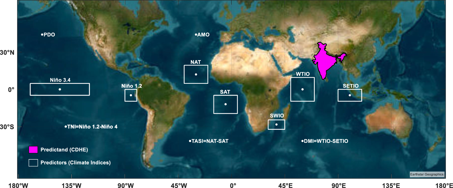
The study focuses on the Indian Summer Monsoon (ISM) period and we utilized the Climatic Research Unit (CRU) gridded monthly precipitation and temperature datasets for the Indian mainland (covering 68° E–98° E longitude and 8° N–37° N latitude) from 1951 to 2020 (Harris et al 2020). CRU has been established as reliable in capturing the spatiotemporal variability of precipitation and temperature over India (Bejagam and Sharma 2022). We examined the oceanic indices from three distinct ocean basins (figure 2) based on previous studies since they have a significant association with the Indian monsoon. These include PDO, Niño 3.4, Niño 1.2, and TNI representing the Pacific Ocean (Hassan and Nayak 2020, Sharma et al 2020, Gupta and Jain 2021, Nagaraj and Srivastav 2023); AMO, NAT, SAT, and TASI representing the Atlantic Ocean (Bhatla et al 2016, Malik et al 2017, Borah et al 2020, Sooraj et al 2023); and SWIO, WTIO, SETIO, and DMI representing the Indian Ocean (Sardana et al 2022, Bajrang et al 2023). The monthly time series of these indices were obtained from Extended Reconstructed Sea Surface Temperature version.5 dataset (Huang et al 2017) (see data availability statement).
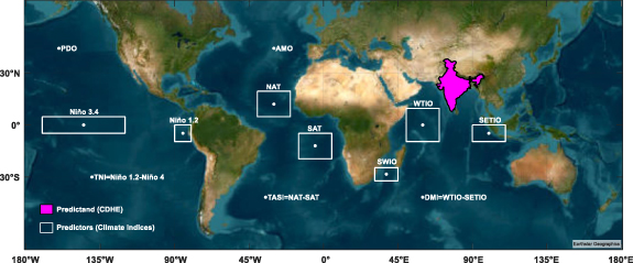
Figure 2. Illustration of the 12 oceanic indices, including the Pacific Decadal Oscillation (PDO), Niño 3.4, Niño 1.2, Trans Niño Index (TNI), Atlantic Multidecadal Oscillation (AMO), North Atlantic Tropical (NAT), Southern Atlantic Tropical (SAT), Tropical Atlantic Index (TAI), Southwestern Indian Ocean (SWIO), Western Tropical Indian Ocean (WTIO), Southeastern Tropical Indian Ocean (SETIO), and Dipole Mode Index (DMI). The white boxes represent the predictors, which are 3 month averaged SST values of the oceanic Index, while the magenta box represents the CDHE, the predictand. Table S1 provides the spatial coverage of each climate index. Readers can refer to Chen et al (2016) for further in-depth insight regarding the indices.
Download figure:
Standard image High-resolution imageIn this study, we aim to do prediction on a seasonal scale (i.e. 2 months in advance). Accordingly, we used the 3 month average SST data of JFM (January–February–March), FMA (February–March–April), MAM (March–April–May), and AMJ (April–May–June) to predict the occurrence of CDHEs in June, July, August, and September, respectively. All the time series were linearly detrended and this is a general practice (Hari et al 2022, Mamalakis et al 2022) to avoid the influence of long-term trends. For discussion, we divided the Indian mainland into ten sub-regions (figure S5) based on previous studies (Guntu et al 2020, 2023, Guntu and Agarwal 2021).
3.2. Relationship between the CDHE and SST anomalies
We calculated the  considering all the 70 year dataset of oceanic indices and CDHE occurrences. However, in the development of prediction model, we employed 10-fold cross-validation instead of 70 year dataset. Findings with statistical significance at a level of 0.05 are only discussed. In June, positive anomalies in the Niño 3.4 region (figure 3(a)) coincided with the occurrence of CDHEs in Eastern, Western, and North-western India. Similarly, positive anomalies in the other Pacific Ocean indices (figure S7) and DMI (figure 3(i)) were associated with CDHE occurrences in Eastern India. While a negative AMO anomaly coincided with 40% of CDHEs in North-central India (figure 4(e)). Moving to July, a positive Niño 1.2 anomaly (figure S7(f)), coincided with the occurrence of CDHEs in the North-central India and South-central India. Furthermore, positive SETIO anomaly (figure S9(j)) and negative AMO anomaly (figure 4(f)) were linked to CDHEs in South-central India. In the important August month, a positive anomaly in the Pacific Ocean (figures 3(c) and S7) coincided with 40% of CDHEs in Western India and North-western India. Additionally, a positive AMO anomaly (figure 3(g)) was associated with CDHE occurrences over North-eastern India, while positive anomalies in other Atlantic indices (figure S8) were linked to CDHE events in North-western India. Lastly, in September, a positive anomaly in the Atlantic Ocean (figures 3(h) and S8) coincided with the CDHE events in North-western India. A positive DMI anomaly (figure 3(l)) was linked to 40% of CDHEs in North-central India, while negative DMI (figure 4(l)) was associated with CDHEs over North-western India.

Figure 3. Conditional precursor coincidence rate between CDHE and positive SST anomalies of Nino3.4 (top panel: (a)–(d)), AMO (middle panel: (e)–(h)), DMI (bottom panel: (i)–(l)) during June, July, August and September. The impact of positive SST anomalies on CDHE reveals diverse teleconnections contributing to CDHE occurrences across different regions of the country.
Download figure:
Standard image High-resolution image
Figure 4. Conditional precursor coincidence rate between CDHE and negative SST anomalies of Nino3.4 (top panel: (a)–(d)), AMO (middle panel: (e)–(h)), DMI (bottom panel: (i)–(l)) during June, July, August and September.
Download figure:
Standard image High-resolution imageOur results are in line with the driving mechanism identified by the previous studies. For instance, Niño 3.4 is widely recognized for its global climatic influence, including in India (Gupta and Jain 2021), where positive anomalies indicate warmer SST in the central and eastern equatorial Pacific, triggering atmospheric changes leading to CDHE events. Krishnamurthy and Krishnamurthy (2014), established a robust correlation between the warm phase of the Pacific Ocean and the droughts in Eastern India. The warm temperature triggers changes in the atmospheric circulation patterns, weakening the walker circulation due to the high-pressure system over Darwin (Pandey et al 2020). Similarly, a warm phase in the Niño 3.4 and PDO regions has also been linked to droughts in Central India (Nagaraj and Srivastav 2023) and North-western India (Singh et al 2022). Further, a study by van Oldenborgh et al (2021) highlighted that a warm phase in both the Pacific and Indian Ocean leads to arid conditions in Central India. Additionally, Ratna et al (2021) found a strong correlation between the positive phase of the DMI and droughts in Central India. The warm phase in DMI creates a high-pressure system over WTIO, diverting trade winds towards the SETIO region instead of the Indian Mainland (Shah and Mishra 2020). However, Sardana et al (2022) reported that cold phase of DMI can result in dry conditions in North-western India during the monsoon withdrawal period. Furthermore, previous studies (Borah et al 2020, Singh et al 2021, Sooraj et al 2023) consistently revealed a strong association between the cold phase of the Atlantic Ocean and droughts in Central India. The physical mechanism for this teleconnection has been explained by Goswami et al (2006), where a cold phase of NAO changes wind patterns, leading to a decrease in the meridional gradient of tropospheric temperature, resulting in below normal precipitation.
3.3. Identification of predictors
Complexity science is used in this analysis to identify the important predictors contributing to CDHE. The degree (figure 5) illustrates the number of SST indices linked to each predictand node and figures S13–S16 depicts the network during JJAS. In general, a high degree value for a node indicates that the occurrence of CDHE is influenced by SST variability in multiple oceans. Identifying the most significant predictor linked to CDHE occurrences becomes crucial to reduce the influence of multiple predictors. Conversely, grid points with zero degree do not have any predictors. In June, CDHEs in Eastern India and South-central India were linked to positive (figure 5(a)) and negative (figure 5(b)) anomalies of multiple indices. During July (figure 5(c)), North-central India stood out with a high degree, indicating that CDHEs in this region are connected to positive anomalies of multiple climate indices. Meanwhile, CDHEs in North-western India and North-eastern India are linked to negative anomalies (figure 5(d)). In August, CDHEs in North-western India showed a complex relationship characterized by positive and negative anomalies (figures 5(e) and (f)). In contrast, CDHEs in Eastern India, North-eastern India were associated with positive anomalies (figure 5(e)), while Southern India were primarily linked with negative anomalies only (figure 5(f)). CDHEs during September over Western India, North-western India, and South-central India were driven by both positive and negative anomalies (figures 5(g) and (h)).
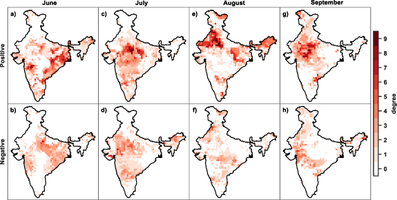
Figure 5. Spatial distribution of node degree values in the CDHE-SST indices network for June (a), (b), July (c), (d), August (e), (f), and September (g), (h), respectively. The top panels represent the connections observed when the SST anomaly is positive, while the bottom panels show the number of connections when the SST anomaly is negative.
Download figure:
Standard image High-resolution imageHowever, it is important to note that one of the assumptions of the logistic regression model is the independence of predictors. Therefore, using multiple predictors can lead to overfitting of the prediction model (Mamalakis et al 2022). Overfitting results in reduced generalization performance, especially when predictors are interdependent (Meyer et al 2019). To address this concern, it becomes crucial to prioritize the identification of the two most significant predictors that exhibit the strongest association with the occurrence of CDHE. Considering only the top two predictors, we can mitigate the risk of overfitting and ensure the development of robust prediction model. Figure 6 shows the top two predictors. Notably, the Pacific Ocean indices emerge as the most important and second most important predictors for the southern and eastern parts of the country during June and July. In July and September, Atlantic Ocean indices plays an important role in driving CDHEs in North-western India and South-central India. In August, it remains the primary driver for South-central India. Further, indices of Indian Ocean is the primary driver for Eastern India during August, while they are secondary for Central India from July to August.

Figure 6. Illustration of the top two predictors associated with CDHE occurrences during (a) June, (b) July, (c) August, and (d) September. The colorbar represents different SST indices, with the first four indices corresponding to the Indian Ocean, the next four indices representing the Atlantic Ocean, and the subsequent four indices representing the Pacific Ocean. In grid points where NaN is indicated, it signifies that none of the SST indices has a significant dependence on the occurrence of CDHE events in that specific location.
Download figure:
Standard image High-resolution image3.4. Predictors skill assessment
The skill of the proposed predictors is examined using the 10-fold cross validation (see section 2.4). For a grid point with two predictors, the model is chosen based on the low BIC value and considered as the best model. By doing so, the multi-collinearity between the two predictors can be mitigated. A similar procedure has been used in Mukherjee et al (2020) and Mamalakis et al (2022). The statistically significant regression coefficients is shown in figure S17. Notably, it validates the findings in section 3.1, consistently identifying positive and negative relationships between the CDHEs and indices. The prediction skill (BSS) is shown in figure S18. The skill (BSS > 0) illustrates that the proposed predictors can perform better compared to reference prediction. Next, to test the accuracy of the model, the probability of CDHE occurrence was estimated for all the years.
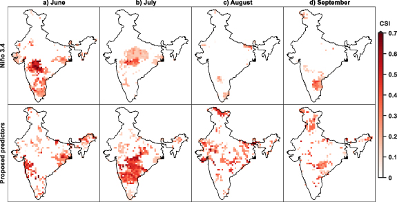
The CSI was computed to gain insight into the accuracy of the proposed predictors compared to stand-alone Niño 3.4 prediction in predicting hits (observed as CDHE). The top panel (figure 7) focuses on the CSI based on Niño 3.4 as a predictor for each month, while the bottom panel displays the CSI based on the proposed predictors. While Niño 3.4 exhibits few grid points with high CSI, the proposed predictors demonstrate higher values for more grid points. For instance, Niño 3.4 prediction in June (figure 7(a)),  were observed in South-central India only. But utilizing the proposed predictors, higher values are also seen in Eastern India, and North-eastern India. Similarly, in July (figure 7(b)), higher CSI is observed in Central India based on Niño 3.4. Meanwhile with the proposed predictors, higher values are also observed in South-central India. The difference is also prominent in August (figure 7(c)) and September (figure 7(d)). Further, FAR (figure S19) also reveal the accuracy of the negative predictions among all the non-CDHE events. Additionally, the range of skill scores are consistent with the leave-one-out cross validation scheme (figure S20). This comparison highlights the accuracy of the proposed indicators and the ability to provide better prediction across different regions compared to stand-alone Niño 3.4 prediction.
Figure 7. Critical Success Index (CSI) for CDHE prediction using different predictors. The top panel depicts the CSI based on Nino 3.4 as a predictor for each month, namely (a) June, (b) July, (c) August, and (d) September. In contrast, the bottom panel display the CSI based on the proposed predictors. Higher CSI values reflect superior prediction performance.
Download figure:
Standard image High-resolution image
4. Conclusions
The combination of ECA and complexity science allows for identifying the most important predictors. The findings highlight distinct spatial patterns of CDHEs, with varying key drivers across seasons and regions. The climate indices in the Pacific Ocean have been determined to be the most important predictor for the Eastern India and Western India. While indices of the Atlantic Ocean are the most important predictor for the Central India, followed by the climate indices of the Indian Ocean. However, other factors such as the land surface conditions (Rajeev et al 2022, Das et al 2022b) and anthropogenic activities can also influence climate in India. For instance, Ambika and Mishra (2019), demonstrated that the irrigation practices considerably modulate land surface temperature in the Indo-Gangetic Plain. Future research can incorporate the above factors to improve the understanding of complex driving mechanisms. Compared to stand-alone Niño 3.4-prediction, the proposed drivers outperform the accuracy of predicting the observed CDHEs. Nevertheless, one of the shortcomings is the use of a 70 year dataset which may introduce high uncertainty compared to longer records (Singh et al 2021), and future research should address this limitation. In summary, the study has two significant contributions. One is the methodological advancement, and the other is the physical understanding of CDHEs during the ISM considering intra-seasonal variability. This study serves as the foundation for predicting the occurrence of CDHE and developing effective adaptation strategies.
Acknowledgments
R K G and A A highly appreciate the APC waiver provided by Environmental Research Letters. R K G gratefully acknowledges the financial support received from the Prime Minister's Research Fellowship (PM-31-22-695-414). R K G and A A would like to acknowledge the joint funding support from the University Grant Commission (UGC) and DAAD under the Indo-German Partnership in Higher Education (IGP2020-24/COPREPARE) framework at the IIT Roorkee. We also extend our thanks to the reviewers for their valuable feedback, which contributed to improving the quality of the manuscript.
Data availability statements
We thank the following agencies for archiving and making data accessible. CRU from university of East Anglia: https://crudata.uea.ac.uk/cru/data/hrg/cru_ts_4.06/ (V4.06 accessed in March 2023); ERSST v5: www1.ncdc.noaa.gov/pub/data/cmb/ersst/v5/netcdf/ (accessed in March 2023). PDO: www.ncei.noaa.gov/pub/data/cmb/ersst/v5/index/ersst.v5.pdo.dat (accessed in March 2023). Software for ECA and Logistic regression is available at https://tocsy.pik-potsdam.de/coincalc.php and https://in.mathworks.com/help/stats/fitglm.html, respectively.
All data that support the findings of this study are included within the article (and any supplementary files).
Conflict of interest
The authors declare no conflicts of interest relevant to this study.
Author contributions
R K G: Funding acquisition, Data curation, Formal analysis, Investigation, Methodology, Conceptualization, Resources, Software, Writing—original draft, Writing—review & editing. A A: Funding acquisition, Conceptualization, Project administration, Supervision, Writing—review & editing.
Supplementary data (30.1 MB PDF)