

Abstract
Global food systems must be a part of strategies for greenhouse gas (GHG) mitigation, optimal water use, and nitrogen pollution reduction. Insights from research in these areas can inform policies to build sustainable food systems yet limited work has been done to build understanding around whether or not sustainability efforts compete with supply chain resilience. This study explores the interplay between food supply resilience and environmental impacts in US cities, within the context of global food systems' contributions to GHG emissions, water use, and nitrogen pollution. Utilizing county-level agricultural data, we assess the water use, GHG emissions, and nitrogen losses of urban food systems across the US, and juxtapose these against food supply resilience, represented by supply chain diversity. Our results highlight that supply chain resilience and sustainability can simultaneously exist and are not necessarily in competition with each other. We also found a significant per capita footprint in the environmental domains across Southern cities, specifically those along the Gulf Coast and southern Great Plains. Food supply chain resilience scores ranged from 0.18 to 0.69, with lower scores in the southwest and Great Plains, while northeastern and Midwestern regions demonstrated higher resilience. We found several cities with high supply chain resilience and moderate or low environmental impacts as well as areas with high impacts and low resilience. This study provides insights into potential trade-offs and opportunities for creating sustainable urban food systems in the US, underscoring the need for strategies that consider both resilience and environmental implications.
Export citation and abstract BibTeX RIS

Original content from this work may be used under the terms of the Creative Commons Attribution 4.0 license. Any further distribution of this work must maintain attribution to the author(s) and the title of the work, journal citation and DOI.
1. Introduction
The global food system accounts for a large proportion of global greenhouse gas (GHG) emissions (Crippa et al 2021), blue water use (Mekonnen and Hoekstra 2020), and nitrogen pollution (Zhang et al 2021) with 5.2 billion tons of CO2 emissions, 1810 km3 of blue water use, and 104 tera-grams of nitrogen applied (Springmann et al 2018). Enhancing the efficiency of food systems in terms of resource use and environmental emissions is essential to meet several sustainable development targets (Springmann et al 2018, Gerten and Kummu 2021). However, food systems face growing environmental challenges, as shown by the rising frequency of climate-related food shocks in recent years (Cottrell et al 2019, Nyström et al 2019). Resilient food systems that can cope with environmental stressors are key to mitigate the impacts on human populations of food supply disruptions, food price fluctuations, and food quality reductions (Davis et al 2021). Urban populations, which comprise 55% of the world's population and consume 75% of the world's natural resources (UN Department of Economic and Social Affairs 2018), are particularly vulnerable to food shocks because they rely on imports from other regions to satisfy local food demand (Davies 2018, Dermody et al 2018). Therefore, building resilient and sustainable food systems for urban areas is crucial to ensure food security, lower environmental impacts, and enhance human well-being (Elmqvist et al 2019).
Measuring the environmental impacts of food systems has the potential to show differences across geographies and time scales and track progress towards certain sustainability goals (Fanzo et al 2021). While studies on the environmental impacts of food systems at the global scale can help us understand how these systems contribute to GHG emissions and planetary resource use (Oita et al 2016, Clark et al 2020, Rosa et al 2020, Crippa et al 2021, Gephart et al 2021, Xu et al 2021), this scale does not allow for deep understanding around the intranational variability of several technological, economic, ecological, and social factors that affect food production and associated environmental emissions. Intranational environmental emission patterns can vary substantially in large countries like the United States (US) (Ahams et al 2017, Mahjabin et al 2018, 2021, Marston et al 2018, Wang et al 2022). Therefore, intranational estimates of environmental impacts could help to inform policies aimed at reducing the environmental impacts of food production.
Environmental extremes and year-to-year environmental variations are both drivers of shocks to food production systems (Cottrell et al 2019, Davis et al 2021). Motivated by ecological theory, studies have shown that biodiversity increases ecosystem productivity, resulting in more stable crop yields over time (Renard and Tilman 2019). Research has also found that the structure of the global food trade network is linked to the system's ability to respond to food consumption supply shocks. Specifically, when the network's modularity decreases this ability of the system to respond to shocks is reduced (Puma et al 2015, Tu et al 2019). The increase in the connectivity of the global food trade network have led to a higher shock transmission, meaning that a shock starting in one country can affect other countries that depend on that county's food exports to meet their domestic food demands (Bren D'Amour et al 2016, Fader et al 2016, Marchand et al 2016, Gephart et al 2016b, Distefano et al 2018). Further, supply diversity in terms of food products and trading partners has been reported to increase the resilience of national food supply systems (Kummu et al 2020).
Intranational studies investigating food production networks found that landscape diversity and complexity can increase crop productivity and yield (Abson et al 2013, Rotz and Fraser 2015, Burchfield et al 2019, Nelson and Burchfield 2021). Similarly, cities with diverse food supply chains are less likely to experience shocks because they possess a functional redundancy of trading partners where a city has multiple trading partners within several functional groups (Gomez et al 2021). However, this may pose a trade-off between resilience and environmental impacts of cities' food systems because having multiple trading partners may result in increased GHG emissions related to food transportation, higher water consumption from trading partners with irrigation systems, N and P loss due to spatial differences in the application of fertilizers for crop and feed production.
Resilience and sustainability are complementary but not interchangeable concepts (Elmqvist et al 2019). The focus of sustainability efforts is on avoiding inefficiencies through the optimization of existing infrastructure and resources, which in some cases means reducing redundancy, a key characteristic of resilient systems (Walker et al 2004, Elmqvist et al 2019). Resilience does not necessarily imply sustainability, and in some cases, it can even undermine it. For example, a resilient city may persist in an unsustainable state by outsourcing food production to other regions with inefficient resource use and large environmental emissions. Thus, it is key to consider both these characteristics to assess the suitability of urban food systems.
The objective of this study is to explore the relationship between resilience and the environmental impacts of major US cities. Resilience and environmental impacts are not necessarily independent from each other, because the resilience of a city may depend on its ability to cope with external shocks and stresses that affect its food supply, such as environmental extreme events or geopolitical conflicts. In putting safeguards in place to adapt to such shocks and stresses, cities may also incur in unsustainable practices with potentially large environmental consequences, such as increasing the carbon or water footprints of their food supply chains. Therefore, we argue that a resilient city should not only be able to maintain its food supply in the face of disturbances, but also minimize its environmental footprint and contribute to the sustainability of the global food system. To support this argument, we develop a framework that integrates indicators of food supply resilience and environmental impacts, and apply it to 69 cities in the United States. We address the following research questions: (1) what cities and food sectors are responsible for the largest food-related environmental impacts in the United States? (2) Does food supply resilience relate to higher food consumption related environmental impacts? (3) What cities exhibit a high food supply resilience while maintaining low environmental impacts, or conversely what cities achieve resilience through increased environmental emissions? To evaluate the environmental impact of US urban food systems, we compare the water use for irrigation, GHG emissions, and N losses using county-level agricultural production data. To assess the resilience of cities to food supply chocks, we leverage supply chain diversity (Gomez et al 2021) as a surrogate for food supply resilience. By examining the relationship between food supply resilience and environmental impacts, we aim to identify potential trade-offs and opportunities for sustainable food systems in US cities.
2. Methods
2.1. Food flow networks
We use annual food flow data at the subnational scale to build food flow networks for 69 major US cities and 3 food sectors. To build the networks, we use data from the Freight Analysis Framework (FAF) version 4 (Hwang et al 2016) which provides annual commodity flows for 132 geographic areas in the US during the 2012–2015 period (figure S27). We use commodity flows to build sectoral food flow networks where nodes represent geographic areas, and the weighted links represent annual food flows for each food sector during 2012–2015 (figure S1). In total, we work with a total of 16 food flow networks (one network for each economic sector and year pair).
2.2. Environmental impacts of food systems
2.2.1. Footprints of production
To assess the environmental impacts of domestic food production we combine county and commodity level production data with environmental footprint factors related to water use, GHGs emissions, and nitrogen leaching. We obtain the state-level water use coefficients [m3 tons−1] for individual crops and livestock from (Mekonnen and Hoekstra 2011) and (Mubako 2011). We use life cycle GHG emission coefficients [kg CO2eq/kg] for individual crops which are obtained from a meta-analysis of published literature (Petersson et al 2021). GHG emission coefficients for North America and for different live animals are adopted from the Global Livestock Environmental Assessment Model version 2.0 from the Food and Agriculture Organization (FAO 2018). GHG emission coefficients account for CO2, N2O, and CH4 emissions. Nitrogen loss coefficients [kg N lost/kg] from crop and livestock production in the US are obtained from (Gephart et al 2016a). In our analysis, commodity-specific environmental coefficients for GHG emissions and nitrogen loss do not vary spatially which is similar to other national level studies (Leach et al 2012, Gephart et al 2016a). This assumption is justifiable as the use of fertilizer and other inputs do not vary widely within many industrialized countries (Leach et al 2012, FAO 2018). Environmental footprint factors and additional processing methods for calculating county level data from the FAF framework are shown in the supplementary information (figures S2–S19 and tables S1–S7).
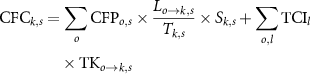
We calculate water (WFP), carbon (CFP), and nitrogen (NFP) footprints for a county i and sector c as
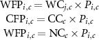
where  is the production of commodity c at county i,
  is the water use coefficient for commodity c at state j,
  is the carbon emission coefficient for commodity c, and
  is nitrogen lost coefficient for commodity c. Environmental footprints for cereal grains, feed, and meat sectors are calculated by aggregating commodity-specific footprints at each county as
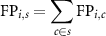
where  is an environmental footprint (WFP, CFP or NFP) for county i and sector s,
  is an environmental footprint for county i and commodity c. Maps of county- and sector-level WFP, CFP, and NFP are shown in the supplementary information. We further aggregate footprints to the FAF scale by summing county-level footprints to FAF zones as
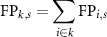
where  is an environmental footprint (WFP, CFP or NFP) for FAF zone k and sector s. Maps of FAF- and sector-level WFP, CFP, and NFP are shown in the supplementary information.
2.2.2. Footprints of consumption
To calculate footprints of consumption we use food flow networks to distribute the environmental impacts of food production to places where food is transferred for consumption. We calculate water footprint of consumption (WFC) for FAF zone k and sector s as
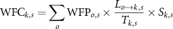
where  is the water footprint of production for origin FAF zone o and sector s,
  is a food flow link between origin FAF zone o and destination FAF zone k, and
  is the total outflow for FAF zone k and sector s.
  is the share of the total production in sector s in FAF zone k that is transferred domestically. We use FAF data to calculate
  and is calculated as the ratio of domestic production to total production (including exports) for sector s in FAF zone k. We calculate the carbon footprint of consumption (CFC) for FAF zone k and sector s in a similar way, but we add a term to the equation to account for GHG emissions involved in the transportation of food products as
where  is the carbon footprint of production for origin FAF zone o and sector s.
  is the transportation GHG emission intensity for transportation mode l (table S7) and
  is the tonne-km of freight transportation for sector s from origin FAF zone o and destination FAF zone k. Tonne-km data is provided in the FAF data. Our method to calculate CFC builds on a previous carbon footprint study (Xu et al
2021). Lastly, the nitrogen footprint of consumption (NFC) of FAF zone k and sector s is calculated as
is the tonne-km of freight transportation for sector s from origin FAF zone o and destination FAF zone k. Tonne-km data is provided in the FAF data. Our method to calculate CFC builds on a previous carbon footprint study (Xu et al
2021). Lastly, the nitrogen footprint of consumption (NFC) of FAF zone k and sector s is calculated as
where  is the nitrogen footprint of production for origin FAF zone o and sector s. Our method to calculate consumption footprint accounts for the spatial variation of food production and its environmental impacts, as well as the outsourcing patterns of cities. The water, GHG, and N production footprints of food products vary across regions, depending on the type and intensity of food production (figures S12, S15 and S18). Different regions specialize in different food commodities, which have different emission factors and water requirements. Thus, the environmental consumption footprints of cities depend not only on the trade data, but also on the environmental footprint of the source regions.
2.3. Food supply resilience
We use the approach in (Gomez et al
2021) to calculate the food supply resilience of 69 major US cities. In this study, we use supply chain diversity as a proxy for resilience because a higher supply chain diversity relates to a lower probability of experiencing food supply shocks of increasing intensity (Gomez et al
2021). Thus, we are using the definition of resilience from the social-ecological system literature, which is 'resilience is the capacity of a social-ecological system to absorb or withstand perturbations and other stressors such that the system remains within the same regime, essentially maintaining its structure and functions.' (Holling 1973, Walker et al
2004). To compute food supply resilience, we analyze separately the annual food supply subnetwork of each city and food sector. For each subnetwork, we calculate the distance between node i (city under analysis) and all neighbors j in the functional space constituted by five functional indicators: physical distance, climate correlation, urban classification, economic specialization, and network modularity. The functional distance  between nodes i and j for each indicator r is then normalized from 0 to 1 such that
  indicates that nodes i and j are the most dissimilar in the network in terms of distance indicator r. To capture a global measure of functional distance between a pair of nodes, we calculate a composite functional distance indicator
  as the arithmetic average across all five indicators. Then, we calculate the food supply resilience
  of city i, food sector c, and year t as the Shannon entropy of the discrete distribution of food inflows by average functional distance category. The discrete distribution of city i is constructed by ordering trading partners j into bins of ascending
  and calculating the proportion of total food inflows from trading partners in each bin. The steps for calculating food supply resilience are summarized in the figure S20.
2.4. Composite environmental impact index
We create a single indicator for the environmental impact of food consumption in cities by equally weighting the three footprints of crop and meat consumption. To do so, we normalize (Muthusamy et al 2016) and standardize the footprints from 0 to 1 where a value of 1 means that the city has the highest environmental impact for that footprint type and food sector and a value of 0 means the lowest environmental impact. We consider crop and meat footprints separately in the calculations to consider relative differences. These standardized footprints are averaged to get a composite indicator. A high value implies that the city has, on average, a large WFC, CFC, and NFC across both crops and meat sector. Note that, we do not consider feed footprints in the calculation of the composite index to avoid double counting of the environmental impacts of meat consumption.
3. Results
3.1. Environmental impacts of food production in the US
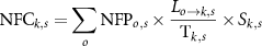
Our findings revealed that meat production had higher environmental impacts than crop production across all three environmental domains, with corn, hay, and beef production contributing the most to these impacts (figure 1). These results align with previous studies that have highlighted the significant environmental footprint of beef production (Capper 2011, Rotz et al 2019). Specifically, the US agricultural sector (crop and meat production) emitted 725.7 million tons of carbon dioxide (Mt CO2eq) in GHG emissions; used 307.7 cubic kilometers (km3) of blue water—surface water and groundwater used for irrigation; and had a nitrogen loss of 8.97 million tons of reactive nitrogen (Mt N). Across all three environmental domains, meat production had higher environmental impacts than crop production (figure 1). Specifically, meat production generated 460.6 Mt CO2eq whereas crop production emissions were 265.1 Mt CO2eq. Similarly, for the other two domains, the water and nitrogen footprints of meat production were 237.6 km3 and 5.6 Mt N while for crop production these are 69.4 km3 and 3.4 Mt N.
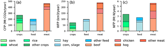
Figure 1. Total environmental footprints of crops, feed, and meat sectors for (a) water, (b) carbon, and (c) nitrogen environmental domains.
Download figure:
Standard image High-resolution imageCorn, hay, and beef production had the highest impacts across all three environmental domains (figure 1). Corn production alone was responsible for 18.4 km3 of blue water use; 132.9 Mt CO2eq in GHG emissions; and 0.78 Mt N of nitrogen loss. These footprints of corn production correspond to 27%, 50%, and 23% of the total water, carbon, and nitrogen footprints of the crops sector.
By examining the spatial distribution of environmental impacts, we found regional patterns in water, carbon, and nitrogen footprints, with some areas experiencing higher impacts than others (figure 2). These regional patterns reflect the varying agricultural production systems and resource use across the US (Capper 2011) where irrigated crops primarily reside west of the Mississippi and meat production is dominant in the central US. These findings affirm the need for region-specific strategies to understand the environmental impacts of food systems, especially in the context of adaptation to climate change (Capper 2011, Mahjabin et al 2021). These results demonstrate variation across indicators which implies that multiple indicators are needed to evaluate the sustainability of agricultural production systems.

Figure 2. Spatial distribution of environmental footprints of production for crops, feed, and meat sectors.
Download figure:
Standard image High-resolution image3.2. Environmental footprints of US urban food systems
Our study focuses on the environmental impacts of food consumption in US cities because cities consume more food than they produce and also account for a large proportion of the food consumed nationally. Food consumption in the 69 cities considered in the study accounts for 277.4 Mt CO2eq in GHG emissions, 129.4 km3 of blue water consumption, and a nitrogen loss of 3.50 Mt N which correspond to 41%, 46%, 42% of the national footprint of consumption of crops and meat.
By combining crop and meat impacts we analyzed the total agricultural consumption footprints for water, carbon, and nitrogen in US cities (figure 3). We do not consider feed impacts when calculating the footprint of agricultural production to avoid double counting. While it is true that food systems contain more food categories, crop and meat products make up nearly 60% of the total food produced in the US.
Figure 3. Environmental footprints of consumption for (a) water, (b) carbon, and (c) nitrogen environmental domains.
Download figure:
Standard image High-resolution imageSouthern cities, particularly those along the Gulf Coast and southern Great Plains, generally have higher per capita footprints across all three environmental domains. Among the top 20 cities with the highest water, carbon, and nitrogen footprints, a significant proportion are in the southern US (18, 11, and 14 respectively; figure S23). Interestingly, the contribution of the meat sector to the total agricultural footprint of production varies among environmental domains (figure S23). For instance, for most cities the meat sector accounts for a larger share of the total water footprint of production than the crop sector but that trend is not universal and there are several places where crop production dominates (figures S23 and S24). Moreover, within the carbon and nitrogen footprints of production, crop and meat sectors have a comparable contribution to the total footprint of production of cities (figures S23 and S24). Southern cities again show high footprints of consumption across all environmental domains. Among the top 20 cities in terms of footprints of consumption, 17, 13 and 13 cities are located in the south for water, carbon and nitrogen footprints of consumption, respectively (figure S23). As expected, the share of the meat sector in the total footprint of consumption of cities is larger than the share for the crop sector across all environmental domains (figures S23 and S24).
3.3. Food supply resilience of US cities
The food supply resilience scores for cities range from 0.18 to 0.69 with an average resilience of 0.46 and standard deviation of 0.12 (figure 4). Cities in the southwest have the lowest food supply resilience of all regions, with an average resilience of 0.39, followed by the Great Plains at 0.41. In contrast, the regions with the highest average resilience are the northeast and Midwest regions, with scores of 0.55 and 0.50, respectively. Among the 69 cities studied, New York City, Kansas City, Atlanta, Richmond, and Philadelphia have the largest food supply resilience. Except for Kansas City all these cities are located in the eastern US. In fact, of the top 25 most resilient cities, 19 are located in the East. On the other hand, cities with the lowest resilience, including Tucson, Corpus Christi, Lake Charles, Beaumont, and Las Vegas, are predominantly located in the western US.
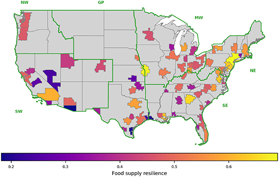
Figure 4. Food supply resilience of US cities. Climate regions (shown in green) are: Northeast (NE), Southeast (SE), Midwest (MW), Great Plains (GP), Northwest (NW), and Southwest (SW).
Download figure:
Standard image High-resolution image3.4. Environmental impacts and resilience of US cities
To answer our second research question, we investigate the relationship between the resilience of supply chains and the environmental impacts embedded in US cities food supplies. Food supply resilience positively relates to the number of trading partners (figure S25) which makes it possible that resilient cities also have larger environmental impacts. However, we find no relationship between food supply resilience and environmental footprints across all environmental domains and food sectors (figure 5). Thus, it is possible for resilient cities to exhibit low and high environmental footprints.
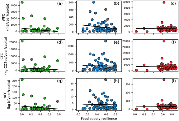
Figure 5. Relationship between environmental footprints and resilience of US cities food supplies across water (a)–(c), carbon (d)–(f), and nitrogen (g)–(i) environmental domains for crops (a), (d), (g), feed (b), (e), (h), and meat (c), (f), (i) sectors. The linear fit to each relationship is shown in black.
Download figure:
Standard image High-resolution imageWe relate the environmental impact indicator to food supply resilience to assess potential tradeoffs where a city might have a resilient food supply at the cost of higher environmental impacts or conversely achieve a high resilience with relatively low environmental impacts (figure 6).

Figure 6. Relationship between food supply resilience and environmental impacts of US cities for crops, feed, and meat sectors.
Download figure:
Standard image High-resolution image
We find that large cities such as New York City, Philadelphia, and Los Angeles exhibit relatively low environmental impacts with a high food supply resilience. The high economic power of these large cities allows them to outsource food to a more diverse set of trading partners increasing their food supply resilience (Bingham et al 2022). In addition, large cities often demonstrate lower consumption footprints per capita across all three environmental domains compared to mid-to small size cities (figures S25 and S26). Cities in the southeast and southern Great Plains regions such as Atlanta, Kansas City, New Orleans, Oklahoma City, and Omaha show a high food supply resilience accompanied by high environmental impacts. The southeast and southern Great Plains regions are characterized by a high environmental impact across all three environmental domains. Medium-to-small sized cities in the Southern Great Plains region such as Wichita, Fresno, and Corpus Christi show large environmental impacts with a low resilience to food supply shocks. For this group of cities, a diversification of trading partners might be beneficial to, both, increase their resilience and decrease their environmental impacts. Lastly, cities in the southwest region such as Tucson, San Diego, and Las Vegas show a low environmental impact and a low food supply resilience.
Part of these finding, the relationship between population and environmental impact efficiency, supports previous research that has demonstrated the potential for large cities to achieve greater efficiency in terms of consumption footprints per capita (Bettencourt et al 2007, 2010, Mahjabin et al 2018). However, we expected to see a relationship between high food supply resilience, and thus higher numbers of trading partners, and higher environmental impacts in the carbon and nitrogen footprint because of the impacts associated with transportation of goods. We did not find that relationship to be present in our work. Thus, this suggests that a higher diversity of trading partners can serve two goals, both reducing environmental impacts and increasing food system resilience.
In summary, our investigation of the resilience of US cities to food supply shocks we found that cities in the southwest had the lowest average resilience, while the northeast and Midwest regions had the highest average resilience. This is important to highlight in the context of providing interventions to improve food supply resilience in regions with lower resilience scores, such as diversifying trading partners (Gomez et al 2021).
3.5. Limitations
In considering limitations, it is important to note that our study investigated the principle of food supply resilience and environmental impacts at an intranational scale thus further research would be necessary to see if the findings would remain true at the global scale where larger environmental impacts are associated with the transport of goods. Beyond this general limitation, several limitations exist within our methodological framework. First, our work utilized annual trade data from the FAF framework thus our conceptualization of resilience is tied to annual timescales. Future work in this area could also explore how major disruption events, such as the COVID-19 pandemic, mirror resilience of supplies by geographic area by using smaller time interval and higher product resolution information. Additionally, given data limitations for calculating each environmental footprint, we only utilized four Standard Classification of Transported Goods (SCTG) commodity groups for this research leaving out three additional food product groups. Thus we did not calculate the entire food supply chain environmental footprints. Further, we considered water, carbon, and nitrogen footprints in this study but further work could elucidate the relationship between resilience and sustainability for other environmental impacts such as land use and biodiversity loss. Land use in particular will remain an important area of consideration for sustainability with competing uses across water, food, and energy systems only growing with expanded deployment of renewable energy and increasing stress on water supplies.
4. Conclusion
Understanding the relationship between cities food supply resilience and environmental impact enables us to build broader context in which to ground discussions of sustainability and resilience. Our study builds understanding around the relationship between food supply resilience and the environmental impacts of urban food systems in US cities, a previously underexplored scale. Our findings highlight the possibility that increasing the number of trading partners a city utilizes might serve two dual purposes- reducing environmental impacts of food systems and improve the food supply resilience across different cities. This work is crucial to informing the development of sustainable urban food systems that can support a growing population while mitigating the environmental impacts of food supply systems.
Acknowledgments
The authors would like to acknowledge the National Science Foundation Grant #1941657 and #2244715, and the George Washington University for providing support for this work.
Data availability statement
All data that support the findings of this study are included within the article (and any supplementary files).
Supplementary data (15.7 MB DOCX)