

Abstract
The transition to electric vehicles (EVs) will impact the climate, the environment, and society in highly significant ways. This study compares EVs to vehicles with internal combustion engines for three major areas: greenhouse gas emissions (GHGs), fuel costs, and transportation energy burden (i.e. percentage of income spent on vehicle fuels). Excluded in the analysis is the purchase cost of the vehicles themselves. The results reveal that over 90% of vehicle-owning U.S. households would see reductions in both GHGs and transportation energy burden by adopting an EV. For 60% of households these savings would be moderate to high (i.e. >2.3 metric tons of CO2e reduction per household annually and >0.6% of energy burden reduction). These reductions are especially pronounced in the American West (e.g. California, Washington) and parts of the Northeast (e.g. New York) primarily due to a varying combination of cleaner electricity grids, lower electricity prices (relative to gas prices), and smaller drive-cycle and temperature-related impacts on fuel efficiency. Moreover, adopting an EV would more than double the percentage of households that enjoy a low transportation energy burden (<2% of income spent on fuel annually). This equates to 80% of all vehicle-owning U.S. households. Nevertheless, over half of the lowest income households would still have a high EV energy burden (>4% income spent on fuel annually), and if at-home charging is unavailable, this rises to over 75 percent. Addressing this inequity hinges on three major interventions: 1) targeted policies to promote energy justice in lower-income communities, including subsidizing charging infrastructure; 2) strategies to reduce electricity costs; and 3) expanding access to low-carbon transport infrastructure (e.g. public transit, biking, and car sharing).
Export citation and abstract BibTeX RIS

Original content from this work may be used under the terms of the Creative Commons Attribution 4.0 license. Any further distribution of this work must maintain attribution to the author(s) and the title of the work, journal citation and DOI.
1. Introduction
Transportation accounts for the largest portion of greenhouse gases (GHGs) emitted in the United States (U.S.), with direct emissions from passenger cars and light-duty trucks comprising roughly 16% of total GHGs alone [1]. Electrification is the primary pathway to reduce these emissions and reaching zero carbon intensity in the transportation sector by 2050 will require complete electrification and decarbonization of the grid [2]. Policies in the U.S., such as the federal-level Inflation Reduction Act ((IRA), which includes electric vehicle (EV)-related incentives) and California's Advanced Clean Cars II rule (which phases out gasoline-powered vehicle sales by 2035), demonstrate momentum for accelerating EV adoption in the U.S.
To better understand the potential benefits and tradeoffs of EVs, extensive research has been conducted. Studies have shown that EV adoption can significantly reduce GHG emissions and other air pollutants depending on the type of EV and geographically variable circumstances such as the source of electricity, driving and charging patterns, charging infrastructure, policies, and climate [3–12]. Numerous studies have explored the regional variability of EV-related GHG emissions in the U.S. [4, 5, 13–26]. The total cost of ownership of EVs versus conventional internal combustion engine vehicles (ICEVs) is also well-studied and debated [27–31], with a few studies assessing the variability of EV costs in U.S. cities [30, 31] or at the state level [22, 32]. There is agreement that EV operating costs (e.g. fuel and maintenance) tend to be lower than those of ICEVs [27, 28, 32–34] and are a key factor in making EVs cost-competitive, in addition to federal tax incentives [28, 29, 31].
Sovacool et al argue that EV research has largely been 'descriptive or positive' and not 'normative or critical' [35, p 205]. Sovacool et al [35, 36] and Dall-Orsoletta et al [37] have evaluated the EV transition using several energy justice tenets, including distributive justice, procedural justice, cosmopolitan justice, and recognition justice [35, 36]. This study centers on the EV transition and distributive justice, which concerns the fair distribution of benefits and burdens. Other tenets are briefly discussed as well.
A frequent focus in energy justice research in the U.S. that falls largely under distributional, procedural, and recognition justice is household energy burden, or the portion of income spent on residential energy services [38]. Consideration of transportation dynamics in energy burden research is particularly lacking in the U.S. [38, 39], but is more prevalent in Europe (e.g. [40–43]), where domestic and transport energy poverty has been coined 'double energy vulnerability' [41]. Transport energy poverty, or transportation energy burden in the U.S. [44–47], is analogous to household energy burden and falls under the larger umbrella of transport poverty [40, 41], or 'the inability to attain a socially- and materially-necessitated level of transport services' [40, p 2]. The U.S. is highly car dependent, with private vehicles representing more than 80% of person trips taken compared to just 2.5% taken via public transit [48]. This underscores the importance of private vehicle affordability in the U.S., particularly where alternative transport modes are not readily accessible or convenient.
A few studies of transportation energy burden in the U.S. have found that low income households [44–47], particularly Black, Latinx, and Native American households [45], face disproportionate burdens. Additionally, suburban and rural households tend to experience higher transportation energy burdens than do urban households [40, 44–47], primarily due to lack of public transit and greater distances to essential services and employment locations [40]. A recent justice–focused analysis found that adopting EVs in the state of Illinois can reduce regional differences in transportation energy vulnerability [47].
However, potential patterns of EV energy burdens, which fall under distributional justice, have not been investigated for the entire U.S., nor have any studies assessed how and where EV energy burdens relate to GHG emissions. This study addresses this research gap by using a spatial model to evaluate three essential factors associated with the EV transition: transportation energy burden, fuel costs, and GHG emissions. We focus on the following questions:
- (a)Where and to what extent do new battery EVs (BEVs) and ICEVs reduce current transportation energy burdens and how do these outcomes vary across income groups?
- (b)Relative to new ICEVs, where and to what extent do BEVs reduce GHG emissions in addition to transportation energy burdens?
To answer these questions, we calculated census tract-level transportation energy burdens and life cycle GHG emissions of new BEV and ICEV models using a spatially explicit approach. We compared new BEV and ICEV energy burdens to transportation energy burdens of the current on-road vehicle stock [44]. Then we compared the spatial variation and extent of energy burdens and GHG emissions for new BEVs and ICEVs.
2. Methods
This study drew on data and methods from previous EV and transportation energy burden research, including vehicle parameters and GHG emissions [4, 5], travel behavior and transportation energy burden [44], and vehicle fuel costs [32]. For GHG emission and fuel cost comparisons, we used 2020 vehicle models for two powertrains (ICEV and BEV) and three vehicle classes (i.e. sedan, sport utility vehicle (SUV), and pickup truck) and assumed that households would switch to the same vehicle class (e.g. sedan ICEV to sedan BEV). To ensure comparability, we applied vehicle and travel behavior parameters consistently across the calculations. The geographic scope of the study is the United States, excluding territories (e.g. Puerto Rico). See the Supplementary Information and online data repository for additional details [49]. 1
2.1. Fuel costs
For fuel cost calculations, we modified data and methods from Borlaug et al [32] by including different vehicle parameters, county instead of state level fuel prices, and more recent data. For each combination of powertrain, vehicle class, and county, we calculated the fuel cost factor ( ) in terms of U.S. dollars per mile (USD mile−1), which reflects lifetime vehicle fuel costs divided by the lifetime vehicle miles traveled (VMT) of the vehicle (
 ):
):
where  is the lifespan of the vehicle (years) [4, 5],
  is annual vehicle VMT for year
  [4, 5, 50] (see S1.2),
  is fuel consumption (gallon or kilowatt-hour [kWh] mile−1) [4, 5, 51–53] (see S1.4),
  is the cost of fuel (U.S. dollars [USD] gallon−1 or kWh−1) [32, 44, 54–56] (see S1.7),
  is the fuel price projection for year
  [57] (see S1.7.2),
  is the charging efficiency (only applicable to BEVs) [4, 5], and
  is the discount rate [32, 58]. Since the cost of charging an EV is influenced by factors such as charging location, time of day, and power level [32], we calculated the levelized cost of charging ((LCOC); in USD kWh−1) instead of simply using electricity prices (see S1.7.1).
Price projections indexed to 2020 ( ) from the U.S. Energy Information Administration (EIA)'s 2021 Annual Energy Outlook [57] were used to calculate fuel prices from 2022 to 2050 (see S1.7.2). We used three projection scenarios in the scenario analysis, as detailed in table 1. LCOC prices for 2020 used EIA data (2019, 2020) and the Utility Rate Database (2013–2022). Gas prices were February 2020 data from GasBuddy via [44]. These gas prices were used to align with the electricity price time frame, as well as the finer spatial resolution compared to EIA sources. February 2020 gas prices are relatively representative of the preceding five years and pre-date more recent price volatility caused by the COVID-19 pandemic, Ukraine war, and other current events (see S1.13).
Table 1. Parameter assumptions for four scenarios. Further details are in the supplementary information.
| Parameter | Variable | Baseline—residential | Baseline—public | Best case for BEV | Worst case for BEV | Source |
|---|---|---|---|---|---|---|
| Lifetime VMT |

| Baseline | Baseline | +20% BEV lifetime | −20% BEV lifetime | [4, 5] |
| Annual vehicle VMT by age |

| Baseline | Baseline | Baseline | Baseline | [4, 5, 50] |
| Fuel consumption |

| Baseline | Baseline | Baseline | Baseline | [4, 5, 51–53] |
| BEV charging efficiency |

| Baseline (85%) | Baseline (85%) | +10% (93.5%) | −10% (76.5%) | [4, 5] |
| Gasoline price |

| Baseline | Baseline | Baseline | Baseline | [44] |
| LCOC |

| Moderate | Moderate | Low | High | This study, [32, 56] |
| Charge Mix | 81% res, 14% pub, 5% DCFC | 40% pub, 60% DCFC | 100% res L1 | 100% DCFC | [32, 77] | |
| EVSE costs | Moderate | Moderate | None | High + grid upgrade |
| |
| O&M costs | 8% | 8% | 1% | 12% |
| |
| Electricity prices | EIA & URDB residential & commercial | EIA & URDB commercial | EIA & URDB residential | URDB commercial | [54, 55] | |
| EIA fuel price projection |

| Reference | Reference | High oil price | Low oil price | [57] |
| Discount rate |

| 3.5% | 3.5% | 3.0% | 7.0% | [32, 58] |
| Vehicle cycle emissions |

| Baseline | Baseline | Baseline | Baseline | [4, 5] |
| Gasoline emissions factor (kg CO2e gallon−1) |

| Baseline (10.67) | Baseline (10.67) | +10% (11.74) | −10% (9.60) | [4, 5] |
| Electric grid emissions factor (NREL Cambium Standard Scenarios) |

| Mid case—no new policy | Mid case—no new policy | Mid case—95% decarbonization by 2035 | High renewable energy costs | [59, 60] |
a Indicates parameter included in sensitivity analysis. Note that BEV and ICEV values were included for lifetime VMT, fuel consumption, and the EIA fuel price projection, bringing the total number of tested parameters to 12. b Source: Based on email correspondence with Borlaug, National Renewable Energy Laboratory (NREL), on 24 May and 25 2022. c U.S. EIA fuel price projections are for motor gasoline and residential electricity (baseline-residential and best case) or commercial electricity (baseline-public and worst case).BEV = battery electric vehicle; DCFC = direct current fast charging; EIA = Energy Information Administration; EVSE = electric vehicle supply equipment; kg CO2e gallon−1 = kilograms of carbon dioxide equivalent per gallon; L1 = level 1 (charging); LCOC = levelized cost of charging; NREL = National Renewable Energy Laboratory; O&M = operations and maintenance; pub = public; res = residential; URDB = Utility Rate Database; VMT = vehicle miles traveled.
2.2. GHG emissions
For GHG emissions, we modified data and methods from Woody et al [4, 5] by adding Alaska and Hawaii and using one different decarbonization scenario. For each combination of powertrain, vehicle class, and county, we calculated the life cycle emissions factor ( ) in terms of grams of carbon dioxide equivalents per mile (gCO2e mile−1), which reflects cradle-to-grave lifecycle GHG emissions of the vehicle divided by the lifetime vehicle VMT:
where  is vehicle cycle emissions (gCO2e) [4, 5] and
  is the fuel emissions factor (gCO2e gallon−1 or kWh−1), which varies by year
  for electricity only [4, 5, 59, 60] (see S1.8). The remaining variables are the same as those in equation (1).
2.3. Household and tract-level results
Figure 1 displays the variables used to calculate household transportation energy burdens and GHG emissions at the census tract level. Zhou et al [44] estimated travel behavior (i.e. annual household VMT) at the census tract level for 220 different household classifications (defined by income, workers, and vehicles) (see S1.3). We filtered out zero vehicle households (approximately 9% of U.S. households) from the dataset and multiplied the county-level  and
and  values by corresponding annual household VMT to calculate annual household fuel costs and GHG emissions at the tract-household classification level.
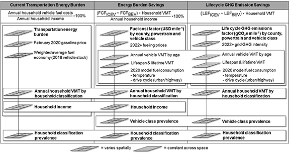
Figure 1. Graphic representation of variables included in this study. BEV = battery electric vehicle; FCF = fuel cost factor; GHG = greenhouse gas; ICEV = internal combustion engine vehicle; LCOC = levelized cost of charging; LEF = life cycle emissions factor; USD = U.S. dollars; VMT = vehicle miles traveled.
Download figure:
Standard image High-resolution imageTo evaluate the transportation energy burden of a new ICEV or BEV using the ratio indicator, we divided the annual household fuel costs by household income:
'Energy burden savings' refers to the difference between ICEV and BEV burdens, while 'GHG savings' refers to GHG emission reductions from adopting a BEV. 'Current transportation energy burden' refers to household vehicle fuel burdens calculated by Zhou et al [44] using February 2020 gas prices and weighted fuel economies of the current on-road vehicle stock (as of 2018), which consisted primarily of ICEVs.
Since the results include multiple vehicle classes and household classifications for each census tract, we aggregated them to facilitate analysis and reporting. We weighted results for the three vehicle classes by prevalence in the tract, based on the 2017 National Household Travel Survey [44, 50] (see S1.5). Likewise, we weighted results for the 220 household classifications by prevalence and aggregated to tract-level. We used a population-weighted average for reporting national-level results. Energy burden for households with varying income levels is somewhat obscured at the aggregated tract level, so our main unit of analysis for transportation energy burden is at the tract-income bin level, aligning with the U.S. Department of Energy's Low-Income Energy Affordability Data Tool [61]. For each tract, we aggregated the results to seven income bins based on area median income (AMI, see S1.6) [62, 63]: 0%–30% AMI, 30%–60% AMI, 60%–80% AMI, 80%–100% AMI, 100%–150% AMI, 150%–200% AMI, and 200%+ AMI.
2.4. Categorizing results
Extensive research has been conducted on housing and transportation affordability (e.g. [64–66]), including household and transport energy affordability (e.g. [42, 44–47, 67–69]) and their appropriate indicators (e.g. [42, 70–72]). When using the ratio indicator, common thresholds for household energy burden (poverty) are 6% and 10% [42, 67–69, 73]. To the best of the authors' knowledge, there is no equivalent threshold for transportation energy burden. Within the U.S. context, the Center for Neighborhood Technology recommends 15% as a transportation affordability threshold [66]. Between 1999 and 2021, fuel and motor oil spending accounted for between 15.1 and 32.8% of U.S. household transportation costs [74]. Therefore, for transportation energy burden, 2.3% to 4.9% is a reasonable range for the unaffordability threshold.
To compare across GHG and energy burden savings, we categorized the tract-level results based on their percentile ranking: 'low' (⩽25th percentile), 'moderate' (>25th percentile and ⩽75th percentile), or 'high' (>75th percentile). Tract-income bin level analysis revealed that current transportation energy burden above 3.9% is 'high,' and below 1.8% is 'low.' We rounded these values up to 4% and 2%, respectively. The high threshold of 4% used in this study aligns well with our estimate of 2.3% to 4.9% described above.
2.5. Scenario and sensitivity analyses
We conducted scenario and sensitivity analyses to assess the models and their parameters. We ran four scenarios (table 1): one baseline representing primarily residential charging ('baseline-residential charging'), another baseline representing public without at-home charging ('baseline-public charging'), one worst-case for BEVs, and one best-case for BEVs.
We included the baseline-public charging scenario because research has shown that interrelated factors such as housing type, housing tenure, and household income impact access to EV charging, with renters, households living in multi-family dwellings, and lower income households less likely to have access to residential EV charging [75, 76]. The calculated LCOC may not always reflect real-world public charging costs, which are affected by EV supply equipment (EVSE) costs, profit margins, and built-in incentives (e.g. free charging); rather, LCOC is intended to reflect the true cost of charging [32].
For the baseline–residential charging scenario, we conducted a parametric sensitivity analysis for 12 parameters (see footnote a in table 1), adjusting each ±10% while keeping the others unchanged. We then calculated the percent change in the results; a change greater than 10% indicates the model is relatively sensitive to the parameter.
3. Results
This section focuses primarily on results from the baseline-residential charging scenario. However, we also briefly summarize results of the baseline-public charging scenario in section 3.1.3 and the worst case and best-case scenarios in section 3.4.
Over 90% of households see some level of savings for both GHG emissions and energy burden, confirming the potential for widespread co-benefits from EV adoption. New BEVs generally reduce current transportation energy burdens significantly more than new (more fuel efficient) ICEVs; however, over half of the lowest income households continue to experience high BEV energy burdens. The scenario analysis indicates that future grid decarbonization, current and future fuel prices, and charging accessibility will impact the extent to which EV benefits can be realized.
3.1. Changes in transportation energy burden
National average transportation energy burden results are presented in table 2. Our analysis of data from Zhou et al [44] indicates that the national average energy burden of the current vehicle stock is 3.6%. As expected, in the baseline-residential charging scenario, adopting new BEVs or new ICEVs would result in lower national average energy burdens. Furthermore, national average energy burdens of a new BEV (1.4%–2% depending on vehicle class) are lower than those of a new ICEV (2.3%–3.4% depending on vehicle class).
Table 2. Population-weighted national average transportation energy burdens for the baseline-residential charging scenario. BEV = battery electric vehicle; ICEV = internal combustion engine vehicle; SUV = sport utility vehicle.
| Transportation energy burden (%) | |||
|---|---|---|---|
| Vehicle class | Current on-road vehicle stock | New BEV | New ICEV |
| Sedan | 3.6 | 1.4 | 2.3 |
| SUV | 1.7 | 2.7 | |
| Truck | 2.0 | 3.4 | |
3.1.1. Tract-level results
Current vehicle stock and new ICEV burdens are moderate for most census tracts (figures 2(a) and (d)), while BEV burdens for most tracts are low (figure 2(b)). New BEV adoption results in average fuel cost reductions of 55%, with 71% of households seeing over a 50% reduction in fuel costs (figure 2(c)). By comparison, new ICEV adoption results in average fuel cost reductions of 27%, with only 0.02% of households seeing over a 50% reduction (figure 2(e)).
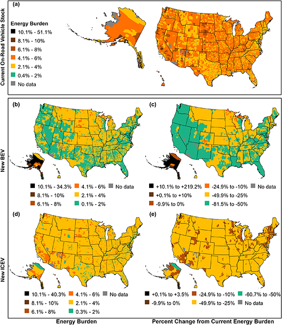
Figure 2. Geographic distribution of average transportation energy burdens, census tract level. (a) Energy burdens for the current on-road vehicle stock from [44]. (b)–(e) Energy burdens and percent changes from current energy burdens for a new BEV and a new ICEV. BEV = battery electric vehicle; ICEV = internal combustion engine vehicle.
Download figure:
Standard image High-resolution imageThe greatest fuel cost reductions (50%–81%) from adopting a BEV occur in the American South and West, while increases in energy burdens (as much as 219%) occur for a very small percentage of households (0.1%) living in Alaska, Michigan, Maine, Rhode Island, and Massachusetts (figure 2(c)). Areas with high BEV energy burden reductions have either lower LCOC relative to gasoline prices, relatively smaller temperature and drive cycle-related impacts on fuel consumption, or both (figures S9 and S11–S14).
3.1.2. Results by income (tract-level)
While around 33% of households currently have low transportation energy burdens, fuel cost reductions from BEV adoption are significant enough that more than double the American households (i.e. over 80%) would have low BEV energy burdens (figure 3). Moreover, the percentage of high burden households drops by almost two-thirds to 7%.
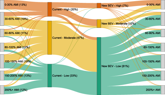
Figure 3. Change in high, moderate, and low energy burden households from the current vehicle stock [44] to a new BEV. The seven income bins are shown on the far left and far right to show the change in household distribution for each income level. AMI = area median income; BEV = battery electric vehicle.
Download figure:
Standard image High-resolution imageHowever, as expected, the lowest income households continue to experience the highest burdens (figure 3). While households with incomes 30%–80% of AMI would have low to moderate BEV energy burdens, with very few still experiencing high burdens, the opposite is true for households with incomes less than 30% of AMI: essentially all would experience moderate (42%) or high (54%) BEV burdens; very few (4%) would experience low BEV burdens.
In most tracts, 0%–30% AMI households experience current transportation energy burdens above 10% that range as high as 95% (figure 4(a)). BEV adoption would significantly reduce burdens overall. Most households with high BEV energy burden have burdens below 6%; very high BEV burdens ranging from 10%–64% are concentrated in the Midwest, Alaska, and Hawaii (figure 4(c)). Around 22% of high BEV burden tracts are urban (24% of households), while the remaining 78% of high BEV burden tracts are suburban or rural (76% of households).

Figure 4. Transportation energy burdens of low-income households. (a)–(d) Geographic distribution of current [44] and BEV energy burdens for low-income households (<60% AMI). (e) Boxplots of BEV energy burdens by state for households with 0%–30% and 30%–60% AMI. States are sorted by median 0%–30% AMI burdens. Whisker represents 1.5 times the interquartile range (note: extent of top whisker for Alaska is cut off for readability). Outliers are not shown. AMI = area median income; BEV = battery electric vehicle.
Download figure:
Standard image High-resolution imageOverall, transportation energy burdens are reduced as incomes increase; most 30%–60% AMI households have low or moderate BEV energy burdens, with the lowest burdens concentrated in the West and Southeast regions (figures 4(d) and (e)). Alaska is a notable outlier for BEV energy burdens, with a median of 13.3% for 0%–30% AMI households and 4.2% for 30%–60% AMI households (figure 4(e)). For 0%–30% AMI households in all other states, median BEV energy burden stays below 10% and drops below the high burden threshold of 4% starting with Washington (figure 4(e)).
3.1.3. Charging access
Aligning with findings from Borlaug et al [32], the true levelized cost of public charging (i.e. Level 2 and direct current fast charging (DCFC)) is higher than residential charging, largely because of the higher EVSE costs. Median baseline-public LCOC is 0.22 USD kWh−1, while the baseline-residential LCOC is 0.16 USD kWh−1 (figure 5(a); also see S1.9). Therefore, in the baseline-public charging scenario, BEV energy burdens are higher and follow the same low income-high burden pattern (figure 5(b)), with over three quarters (77%) of the lowest income households experiencing high BEV energy burdens. Notably, BEV energy burdens in the baseline-public charging scenario are generally still lower than new ICEV and current energy burdens (figure 5(b)).
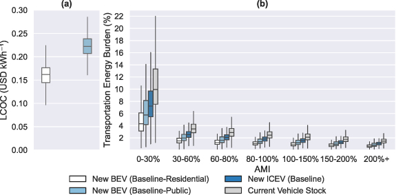
Figure 5. LCOC and energy burden results for a new BEV and ICEV in the two baseline scenarios. Current on-road vehicle stock included for comparison. (a) Boxplots of LCOC (U.S. dollars per kilowatt-hour [USD kWh−1]). (b) Boxplots of energy burden by income bin. Whiskers represent 1.5 times the interquartile range. Outliers are not shown. Note: ICEV assumptions are the same across baseline scenarios. AMI = area median income; BEV = battery electric vehicle; ICEV = internal combustion engine vehicle; LCOC = levelized cost of charging.
Download figure:
Standard image High-resolution image3.2. Geographic distribution of household GHG and energy burden savings
By purchasing a new BEV instead of an ICEV, households in tracts with high annual savings potential would see GHG savings of more than 4.1 metric tons CO2e (tCO2e) household-year−1 (figure 6(b)) and energy burden savings of more than 1.3% (figure 6(c); $595 or more). On the other hand, we delineate low GHG savings potential by 2.3 tCO2e household-year−1 or less (figure 6(b)) and low energy burden savings potential by 0.6% or less (figure 6(c); $273 or less). The remaining tracts fall in between these thresholds in the moderate category.

Figure 6. Geographic distribution of GHG and energy burden savings, census tract level. (a) Bivariate map of GHG and energy burden savings, with the percentage of households in each bivariate category. (b) Geographic distribution and boxplot of potential GHG savings. (c) Geographic distribution and boxplot of potential energy burden savings. (d) Top five states by households in 'Both High,' 'Both Moderate,' and 'Both Low' categories, with boxplots showing the range of GHG and energy burden savings for each state. Whiskers represent 1.5 times the interquartile range. GHG = greenhouse gas; tCO2e = metric tons of carbon dioxide equivalents.
Download figure:
Standard image High-resolution imageOverall, 60% of households live in census tracts with both moderate to high GHG and energy burden savings potential and approximately 91% of households would see some level of GHG and energy burden savings. The category with the most households (27%) is both moderate GHG savings and energy burden savings (figures 6(a) and (d)). Eight percent of households have both high energy burden and GHG reduction potential and are concentrated in the Pacific West, Arizona, and New York ('Both High,' figures 6(a) and (d)). 'Both High' tracts have a combination of one or more of the following factors: smaller impacts on BEV fuel efficiency due to milder temperatures (figures S9(a), (b) and S11), lower electricity prices relative to gas prices (figures S9(c), (d), S12 and S13), current and future electric grids with low carbon intensity (figures S9(e), (f) and S14), higher relative VMT (figure S10(a)), and lower incomes (figure S10(b)). Variations due to VMT and income are mostly observed at regional and local levels (e.g. urban versus suburban and rural).
The remaining portions of the U.S. exhibit low savings potential for either or both factors. Around 8% of households live in 'Both Low' tracts, which are scattered throughout the U.S., with roughly half in the Midwest (figures 6(a) and (d)). Additionally, for one or both factors, there are areas where BEVs and ICEVs perform similarly (i.e. savings are close to zero) 2 and where BEVs definitively perform worse; however, less than 1.3% of households fall into each of these categories. The tracts with low GHG and energy burden savings potential have a combination of one or more of the following factors: greater impacts on fuel efficiency due to extreme cold temperatures (figures S9(a), (b) and S11), higher electricity prices relative to gas prices (figures S9(c), (d), S12 and S13), current and future electric grids with moderate to high carbon intensity (figures S9(e), (f) and S14), lower relative VMT (figure S10(a)), and higher incomes (figure S10(b)).
3.3. Sensitivity analysis
Based on the sensitivity analyses conducted for the baseline-residential charging scenario (see S1.11), the fuel cost model is much more sensitive (figure S15(a)). Most of the parameters result in over 10% changes (±10.9%–29.6% depending on parameter and vehicle class), with ICEV fuel consumption and initial and future gas prices showing the most sensitivity. The GHG model is most sensitive to the gasoline combustion emissions factor and ICEV fuel consumption parameter (at most ±17.2%; figure S15(b)). The other parameters result in less than a 10% change.
3.4. National-level results by scenario and vehicle class
National average absolute values and savings by scenario and vehicle class are illustrated in figure 7. GHG savings range from 1.96 (SUV, worst case) to 6.25 (truck, best case) tCO2e household-year−1. Fuel cost savings range from −700 (truck, worst case) to 1800 USD household-year−1 (truck, best case). Finally, energy burden savings range from −1.5% (truck, worst case) to 3.8% (truck, best case). Negative savings indicate an increase in emissions, costs, or energy burden for a new BEV relative to a new ICEV.

Figure 7. National average GHG emissions (metric tons of carbon dioxide equivalents per household-year [tCO2e hh-yr−1]), fuel costs (U.S. dollars per household-year [USD hh-yr−1]), and energy burden (%), by powertrain and vehicle class for all four scenarios. The colored bars represent the savings (or lack thereof) from a BEV relative to an ICEV. BEV = battery electric vehicle; GHG = greenhouse gas; ICEV = internal combustion engine vehicle; SUV = sport utility vehicle.
Download figure:
Standard image High-resolution imageAlthough savings are generally greatest for the truck vehicle class, the absolute GHG emissions, fuel costs, and energy burdens of a truck are highest of the three vehicle classes. As a result, truck-owning households will experience higher transportation energy burdens and emit more GHGs than sedan and SUV-owning households in the same geographic area (figure 7). In fact, in the baseline-residential charging scenario, average truck energy burdens are 45% and 43% greater than for ICEV and BEV sedans, respectively. Nonetheless, the national-average truck owner that chooses a BEV over an ICEV would have a lower energy burden, as the ICEV transportation energy burdens are around 1.6–1.7 times those of the BEV vehicle classes (figure 7).
Overall, in the worst-case scenario, BEV energy burdens are greater than ICEV burdens for 98% of households (figure S16) due to high-cost DCFC-only charging; however, BEV GHG emissions are greater for only 8% of households that are concentrated primarily in midwest and south–central states (figure S17), where the electric grid remains dominated by fossil fuels due to high renewable energy costs. Research on charging patterns indicates that 100% DCFC charging is unlikely in the real world, while the baseline-public charging scenario is closer to reality for EV owners that do not have reliable at-home charging access [77].
Conversely, in the best-case scenario, BEV fuel costs would be greater than ICEV costs for only 0.07% of households concentrated in Alaska and Maine (figure S16) where high electricity prices and low BEV fuel efficiency persist. All households would see GHG savings (figure S17) due to 95% decarbonization by 2035.
4. Discussion
Our analysis indicates the potential for widespread co-benefits from EV adoption; however, the significant spatial and income-level variation emphasizes the need for regional and localized approaches to address persistent issues of high BEV burden and slow grid decarbonization. Additionally, we consider limitations of the study, including the impact of fuel price and travel behavior uncertainty on our results. Finally, we also briefly discuss our focus on only the distributive tenet of energy justice as it relates to EVs.
Figure 8 provides insights into where cross-sectoral policies are necessary to improve EV benefits. Regions with moderate to high energy burden savings but low GHG savings potential (figure 8(a)) should pursue grid decarbonization policies, while the focus should be more on electricity prices for regions with the opposite trend (figure 8(b)). 'Both Low' areas (figure 8(c)) require both types of policies to increase EV benefits.

Figure 8. Examples of identifying regions for specific policy interventions. (a) Regions where energy burden savings are moderate to high, but GHG savings are low. (b) Regions where energy burden savings are low, but GHG savings are moderate to high. (c) Regions where both energy burden and GHG savings are low. (d) Regions where the lowest income households have high BEV energy burdens. AMI = area median income; BEV = battery electric vehicle; GHG = greenhouse gas.
Download figure:
Standard image High-resolution image
Because high BEV energy burdens are distributed across the U.S. and largely impact lower income households, with the highest burdens in the Midwest, Alaska, and Hawaii (figure 8(d)), localities across the U.S. should consider additional policies to reduce BEV energy burdens alongside EV adoption policies. Since BEVs are more fuel efficient than ICEVs, we must consider the other three factors contributing to transportation energy burden, namely, income, VMT, and fuel prices. Addressing income inequality is a broader discussion point in distributional justice conversations (e.g. [78, 79]); however, this is beyond our scope.
Regarding VMT, approximately 22% of high BEV burden tracts are urban, suggesting an opportunity for reducing energy burden via investment in other transportation modes such as transit, biking, and walking [45, 78]. This same notion can be found in decarbonization literature, which finds that vehicle electrification is unlikely to meet passenger transport mitigation targets alone, and therefore demand–side solutions (e.g. densification, mode switching, behavioral changes) are essential [2, 80–84] and have the potential to reduce emissions by 20%–50% between 2010 and 2050 [82]. Moreover, previous research has identified car infrastructure lock-in and inadequate public transit funding as potential procedural injustices stemming from over-reliance on EV policies to decarbonize passenger transport [35, 36].
The remaining 78% of high BEV burden tracts are suburban or rural and often lack adequate access to alternate transportation modes [85]. This is particularly the case in rural areas where public transit is generally restricted to demand–response transit and less than 1% of people use public transit to commute to work [86]. Increasing access to alternatives, such as transit and car sharing, can alleviate car dependence, but may not be feasible, particularly in rural communities. Reducing high electricity prices is another option, such as through time-of-use and EV-specific electricity rates [32, 87]. For Alaska and Hawaii, which have the highest electricity prices in the U.S., decreasing dependence on oil-fired power is key to reducing costs [88, 89]. Also, a pilot study of pairing rooftop solar and EV incentives indicates promising gains in reducing carbon intensity and electricity prices for low and moderate income households [90]. In addition to reducing electricity prices, ensuring the relative stability of electricity prices, which are generally not subject to the same volatility as gasoline prices, is key to reducing energy price vulnerability for low-income households.
In addition to outstanding transportation energy burden hurdles, the upfront cost of BEVs is a major barrier. Although recent studies have indicated that the total cost of ownership of BEVs can be comparable or less than that of ICEVs, most savings are from lower operating costs and federal incentives [27–29]. We can hypothesize that areas with similar BEV and ICEV fuel costs identified in our study would have higher overall total cost of ownership for BEVs, but this represents an area for future study. Nonetheless, EV ownership in the U.S. has been dominated by households with higher incomes and levels of education [91–93], representing an additional distributional justice concern. This can exacerbate recognition injustice by excluding vulnerable populations (e.g. older and lower income households) from the EV transition [35, 36]. Early EV adoption patterns align with typical trends for most new technologies and while adoption tends to become more equitable over time [79, 94], policy interventions are necessary to increase EV accessibility for vulnerable and excluded households.
Such policies suggested by energy justice scholars include incentives for new and used vehicles, particularly those that are not exclusively tied to taxes [95], programs that specifically target low income households (e.g. California's Enhanced Fleet Modernization Program) [92, 95, 96], and raising awareness about BEVs (e.g. Drive Electric Vermont) [35, 36, 92, 97]. Additionally, increasing access to residential or cheaper public charging is key to addressing distributional justice concerns, particularly for renters, households living in multi-family dwellings, lower income households, and rural households [35, 36, 75, 76].
The 2022 IRA improves the existing federal tax credit program by lifting the cap on manufacturer credits. This allows future adopters the same opportunities as early adopters, and eliminates some barriers for lower and moderate income households, such as limiting eligibility by income and vehicle cost, adding a credit for used vehicles, and allowing credit transfers at point-of-sale [98]. Additionally, the Neighborhood Access and Equity Grants in the IRA provide funding for affordable transportation and other programs in disadvantaged and underserved communities [99] and, as discussed above, could be used to pursue alternative low-carbon transport modes.
Important considerations for our transportation energy burden analysis are the metric's sensitivity to energy prices [42, 100], which was confirmed by our sensitivity analysis, and to travel behavior. While we consider 'high' transportation energy burden to be above 4%, we cannot make any definitive assertions as to whether burdens above this threshold are unaffordable (or vice versa), particularly since we use a modeled approach. Furthermore, our high and low thresholds are derived from 'current' transportation energy burden based on pre-COVID-19 pandemic gasoline prices (February 2020). Our brief analysis indicates that February 2020 prices are relatively representative of the previous five years and August 2022 transportation energy burdens average almost 70% higher than 2020 burdens (see S1.13). Therefore, our estimates of 'current' burden are relatively conservative. The EIA's fuel price projections used for new BEV and ICEV cost estimates are also conservative. Our modeled vehicle lifespans range from 17 to over 18 years and therefore spikes in prices may not significantly impact our results, though sustained increases (or decreases) would, as indicated by the sensitivity analysis. Finally, Zhou et al [44] note that the tract-level annual household VMT is modeled and therefore does not necessarily reflect travel behavior for every household. In fact, the model was found to underestimate VMT for lower income households and overestimate VMT for higher income households. Therefore, our results may underestimate transportation energy burden for lower income households. Overall, these limitations represent areas for further refinement and study.
Sovacool et al applied an energy justice framework to the EV transition [35, 36] to question the notion that the carbon reduction potential renders this transition as 'perpetually positive, neutral, or amoral' [36, p 583]. While our study suggests the significant potential of EVs to reduce GHG emissions and transportation energy burdens, these are just two important considerations within the broader energy justice framework. Though not an exhaustive list, there are other justice concerns related to the EV life cycle that have not been discussed, including upstream activities such as mineral extraction and downstream activities such as battery disposal. The adverse environmental and social impacts associated with cobalt and lithium extraction represent a host of distributional (e.g. concentration in a small number of countries), procedural (e.g. exclusion of indigenous peoples from decision making), and cosmopolitan (e.g. increase in finite resource consumption, toxic pollution, and water scarcity) justice concerns [37]. Battery disposal presents distributional and cosmopolitan justice concerns such as environment, health, and workplace hazards as well as resource depletion. Discussion of life cycle EV-related justice concerns can be found in prior studies (e.g. [35–37, 101]).
5. Conclusion
Our study is the first to jointly consider the spatial variation of EV-related energy burdens and GHG emissions in the U.S. Our results indicate that EVs can significantly reduce energy burdens, particularly more so than new ICEVs, which confirms conjectures in the literature about the transportation energy burden reduction potential of EVs. We have also identified where and how EV energy burdens and GHG emissions vary together spatially, which can better inform location-specific and cross-sectoral electricity and transportation policymaking.
As EV adoption accelerates in the U.S., further justice-focused research is needed. Energy justice scholars highlight that household and transportation energy burdens should be jointly studied, particularly as low-carbon technology diffusion and electrification progresses [40, 43]. Future spatially explicit analyses could use our framework to consider both transportation- and household-related factors (e.g. GHG emissions and air pollution, the total cost of ownership, EV charging infrastructure, urban form, access to vehicles and other transport modes, housing type, race and ethnicity, household energy burdens) to deepen our understanding of how EVs will impact broader transportation and energy justice concerns.
Acknowledgments
CRediT authorship contributions: Jesse Vega-Perkins (conceptualization, data curation, formal analysis, investigation, methodology, project administration, resources, software, validation, visualization, writing—original draft, writing—review & editing); Joshua Newell (conceptualization, methodology, supervision, writing—original draft, writing—review & editing); Gregory Keoleian (conceptualization, methodology, supervision, writing—original draft, writing—review & editing). The authors would like to thank Maxwell Woody at the University of Michigan's Center of Sustainable Systems for his assistance with the life cycle GHG accounting methods; Brennan Borlaug and Michael (Misho) Penev at the National Renewable Energy Laboratory for their assistance with adapting code and methods for the LCOC calculations; and Yan (Joann) Zhou at Argonne National Laboratory for assistance with obtaining more detailed data from the 2020 transportation energy burden study [44]. Finally, the authors are appreciative of feedback provided by the reviewers that enhanced the quality of the article. The authors have no conflict of interests to declare. This study was supported by funding from the University of Michigan's School for Environment and Sustainability.
Data availability statement
The data that support the findings of this study are openly available at the following URL/DOI: 10.17605/OSF.IO/W6CBZ.
Footnotes
- 1
Sections and figures in the Supplementary Information are referenced in this article with 'S' followed by the section or figure number (e.g. S1.1 or figure S9).
- 2
We consider BEVs and ICEVs to perform similarly when GHG emissions and energy burdens are less than 5% different between the two powertrains.
Supplementary information. (3.9 MB PDF) (3.9 MB PDF)