

Abstract
The Arctic has warmed rapidly over the past century, with widespread negative impacts on local and surrounding environments. Previous studies have estimated the overall effects of individual groups of anthropogenic forcing agents on Arctic warming. However, the spatial patterns and temporal variabilities of the separate contributions of greenhouse gases (GHGs), natural forcing agents (NATs; solar radiation and volcanic activity combined) and other anthropogenic (OANT) forcing agents (which are dominated by aerosols) on Arctic land surface air temperatures remain underexamined. Here, we use CMIP6 (the Sixth Phase of the Coupled Model Intercomparison Project) models to quantify the separate contributions of GHGs, NATs and OANT forcing agents to Arctic land surface air temperature changes and analyze their spatial and temporal change patterns from 1915 to 2014. The results show that GHGs alone have warmed the Arctic by 2.72 °C/century (90% confidence interval: 1.42 °C–4.03 °C), 61.8% of which has been offset by OANT agents. The GHG-induced warming peaks are found in Ellesmere Island, Severnaya Zemlya and Svalbard (above 4 °C/century), while the largest cooling effects (above −2 °C/century) induced by OANT agents occurred in Krasnoyarsk Krai and Severnaya Zemlya. A further temporal evolution analysis indicates that the effects of GHGs and OANT forcings have been gradually and robustly detected over time; this increases our confidence in projecting future Arctic climate changes via CMIP6 models.
Export citation and abstract BibTeX RIS

Original content from this work may be used under the terms of the Creative Commons Attribution 4.0 license. Any further distribution of this work must maintain attribution to the author(s) and the title of the work, journal citation and DOI.
1. Introduction
Many studies based on in situ and satellite observations suggest that the Arctic has experienced a significant increase in its near-surface air temperature since the early 20th century (Gillett et al 2008, Box et al 2019, Cai et al 2021, Previdi et al 2021), and the warming rate has more than doubled the global average (You et al 2021). Historical observations also indicate that Arctic warming rates have exhibited a distinct temporal pattern, with a large fluctuation from the early 1890s (1.4 °C/century) to the 2010s (2.1 °C/century) (Huang et al 2019). For example, Chylek et al (2009) reported that two main warming periods and one cooling period occurred from 1910 to 2008 in the high-latitude areas (above 64°N) of the Northern Hemisphere. In addition, Arctic warming has presented evident spatial heterogeneity with larger warming trends (over 6 °C/century) in Severnaya Zemlya, Krasnoyarsk Krai, Franz Josef Land, Svalbard and Novaya Zemlya.
The observed warming over the Arctic has been primarily attributed to the combined effects of greenhouse gases (GHGs) and other anthropogenic influences (Gillett et al 2008, Najafi et al 2015). Based on CMIP5 climate models, Najafi et al (2015) estimated that GHG forcings alone might have warmed the Arctic by 3 °C (90% confidence interval (CI): 2 °C–4 °C) from 1913 to 2012, 1.8 °C (CI: 1.3 °C–2.2 °C) of which has been offset by the cooling effects induced by aerosol forcings, leading to a net warming effect close to the observed warming rate of 1.2 °C (Najafi et al 2015). However, previous attribution studies have mainly focused on the overall effects of anthropogenic factors on Arctic warming without revealing the spatial patterns of their separate contributions. Moreover, previous detection and attribution of Arctic climate change quantify the effects of individual groups of anthropogenic forcing agents for a certain period (Gillet et al 2008, Najafi et al 2015), without revealing the temporal evolution characteristics of the contribution of each anthropogenic forcing agent. Notably, previous studies (e.g. Gillett et al 2008, Najafi et al 2015) may have substantial uncertainties due to the fact that they ignored the effects of model drift when calculating the internal variability (IV) of the complex climate system, which could contaminate the externally forced signals with subsequent impact on the simulated climate change (Gupta et al 2013). Therefore, it is important to revisit this issue by using a more robust detection and attribution method, which is critical to improving our understanding of the causes of Arctic climate change.
To fill above gaps, this study aims to quantify the separate contributions of GHGs, natural forcing agents (NAT, solar and volcanic combined) and other anthropogenic (OANT; dominated by aerosols) forcing agents to Arctic warming rates and, importantly, to examine their spatial and temporal change patterns during the period of 1915‒2014. Based on the Sixth Phase of the Coupled Model Intercomparison Project (CMIP6) climate models, this study adopts a control-simulation approach (CSA) to account for the effects of model drift in our work.
2. Data and methods
2.1. Observed temperature dataset
The Climatic Research Unit gridded time series (CRU) is a widely used climate dataset that covers most land domains worldwide. It is generated through the interpolation of monthly climate observations from more than 4000 weather stations (Harris et al 2020). In this study, the monthly mean temperatures from 1915 to 2014 are adopted from the CRU dataset (version 4.05) at a spatial resolution of 0.5°× 0.5° (https://crudata.uea.acuk/cru/data/hrg/cru_ts_4.05). To further evaluate the robustness of our findings, we repeat our analysis with two additional observational datasets: the Global land average temperature dataset from the University of Delaware (DGLT) and the Goddard Institute for Space Studies (GISS) surface temperature dataset. Detailed introductions of DGLT and GISS can be found in supplementary section 1.
2.2. CMIP6 model simulations
To quantify the effects of natural and anthropogenic forcing agents, we use Arctic temperature simulations by the CMIP6 models driven with historical variations in GHGs, NATs and all forcing agents combined (ALL) (Eyring et al 2016). The OANT forcings are obtained by subtracting the simulations under GHGs and NATs from that under ALL forcing agents. After checking the CMIP6 data archive at https://esgf-node.llnl.gov/projects/cmip6/, only nine models (i.e. ACCESS-CM2, ACCESS-ESM, CanESM5, CESM2, GFDL-ESM4, GISS-E2-1-G, HadGEM3-GC31-LL, MRI-ESM2-0, and NorESM2-LM) provide the required simulations for the period 1915–2014 and are therefore selected for our detection and attribution analysis (supplementary table 1).
Previous studies usually assigned equal weights to each climate model, based on which the ensemble mean is used for analysis. However, different models often show different accuracies, thus pointing to the need for assigning different weights to each model. Here, based on Ridge Regression (RR), we obtain different weights for the nine climate models via building statistical relationship between simulated temperature under ALL forcing and observed temperature (supplementary sections 2, 3 and figure 1). The regression coefficients and weights of the nine models are presented in supplementary table 2. It should be noted that our weighting approach depends on the variable of interest, and it is possible that the CMIP6 models which are good in reproducing observed temperature are poor in terms of other climate variables. Similarly, we build the RR for each pixel and calculate the pixel-level weights of the nine climate models, based on which the multi-model weighted mean is obtained for each pixel. Before training the pixel-level RR, we resampled all model simulations to the resolution of 0.5°× 0.5° to be consistent with the observation dataset based on bilinear interpolation technique.
2.3. Estimation of the internal climate variability
It is well known that changes in temperature are highly affected by naturally generated IV. In this study, we adopt the CSA to estimate the IVs of climate models, based on their preindustrial control simulations with constant external forcings (Resplandy et al 2015, Roberts et al 2015, Olonscheck and Notz 2017).
To obtain more reliable IV estimates, we first remove the least-squares linear trend from each model's preindustrial control simulation to minimize the effect of model drift. Here, the liner trend indicates the trend of each 100 year segment for preindustrial control simulation. We then evaluate the sensitivity of IV to the length of control simulations based on the power spectrum method (supplementary section 4). If the IV given by the control simulation is not equal to the total IV of this particular model, then such models are discarded. After performing the above two steps, a total of 31 032 years of preindustrial control simulations (i.e. piControl) by 48 CMIP6 models (supplementary table 3) are finally used to estimate the IV. We have also calculated the IV based on the nine models used for attribution analysis, though using all available models for calculating IV is well adopted by previous studies (Najafi et al 2015, Mueller et al 2018). Overall, similar estimate of IV is obtained with the relative difference ranging from 2.2% to 5.7% (supplementary figures 2 and 3), suggesting the robustness of our analysis.
2.4. Detection and attribution of temperature changes
In this study, we adopt the well-established approach of total least-squares optimal fingerprinting (TLSOF) technique for the detection and attribution of Arctic land surface air temperature changes to GHGs, NATs and OANT forcings (Hasselmann 1997, Allen and Stott 2003, Stott et al 2010, Hegerl and Zwiers 2011). TLSOF uses a generalized linear regression model, which assumes that the observed Arctic land temperature changes are determined by a linear combination of the covariates (GHGs, NATs and OANT agents) along with a random term. The temperature observations can be expressed as follows:

where  is a vector of observed Arctic land temperature anomalies and
  ,
,  , and
, and  are estimates of the temperature anomalies in response to ALL, NAT and GHG forcings, respectively, with
  indicating the corresponding covariate coefficients. ε is the residual variability that is generated internally in the climate system. Since
  can be decomposed into
  , equation (1) can be rewritten as follows:
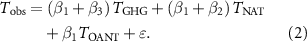
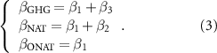
The covariate coefficients associated with GHGs, NATs and OANT forcings, which are referred to as scaling factors, are defined as follows:
Scaling factors are statistically significant if their associated p values are below 10%. If the scaling factors are statistically significant and positive, this suggests that a positive signal is detected in the observations. A negative scaling factor suggests that no physical interpretation can be made or that some important physical processes and other external forcings are not well represented in the climate model (Bindoff et al 2013). If the scaling factors are close to unity, it suggests that the estimated model responses to ALL, NAT and GHG forcings are in accordance with the observed changes.
After estimating the signal amplitudes, we conduct a residual consistency test (RCT) to check whether the estimated regression residuals fit with the climate model noise represented by a second estimate of the IV covariance matrix. After removing all externally forced signals in the regression process, the regression residuals are expected to be consistent with the statistics. An F test is used to compare the variances of regression residuals with the IVs estimated from the control simulations.
2.5. Dynamic evolution analysis of response signals and attributable trends
In this study, a dynamic evolution analysis is used to explore the temporally changing features of the response signals and attributable trends across the Arctic. Specifically, the scaling factors and corresponding attribution trends of GHG, NAT and OANT forcings are calculated for different periods, based on a moving window approach. Here, the 100 year data (1915–2014) are divided into five different time slices (50 year, 60 year, 70 year, 80 year and 90 year), and one year is used as a sliding time window to analyze the dynamic changes in the response signals and attributable trends across the Arctic. A simple schematic diagram of the sliding window approach is presented in supplementary figure 4.
3. Results
3.1. Observed and simulated Arctic land air temperature changes
Figure 1 shows the observed and simulated annual temperature anomalies over the Arctic. The observed average temperature over the Arctic land areas shows a significant warming (p < 0.001) trend (1.20 °C/century) during the period 1915–2014, though a cooling trend from the 1940s to the 1970s and an accelerated warming trend after the 1970s are observed (figure 1). Generally, the climate model simulations under ALL forcings show similar change pattern with the observations, but overestimated the overall trend with a warming rate of 1.53 °C/century (figure 1). As expected, the ensemble weighted mean of simulated temperature under GHG forcings exhibits a monotonically warming trend at a rate of 3.25 °C/century during 1915–2014. The simulated temperatures under NAT forcing exhibit multi-decadal variations without significant change trends (p > 0.05) for the period 1915–2014, though a warming trend is found for the sub-period after 1980s. Under the OANT forcing, a significant (p < 0.001) cooling trend of −1.87 °C/century is detected during the study period 1915–2014.
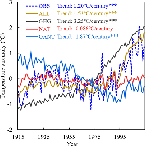
Figure 1. Simulated and observed Arctic temperature anomalies from 1915 to 2014. The observed annual mean Arctic temperature anomalies are compared with 9 model-weighted mean simulated responses to ALL, GHG, NAT and OANT forcings. *** indicates statistical significance at the 0.1% level.
Download figure:
Standard image High-resolution imageSpatially, both the observations and simulations with ALL forcing agents consistently show a warming trend from 1915 to 2014 over the Arctic, with the largest warming effects (above 2 °C/century) found in Chukotka, Ellesmere Island and Svalbard (figures 2(a)–(c)). The multimodel weighted mean responses of temperature to GHG forcings exhibit a larger warming trend than that of the observations (figure 2(c)). The GHG forcings alone contributed the most to the warming trend in the Arctic, especially at Bank Island, Severnaya Zemlya, Novaya Zemlya and Svalbard, with a GHG-induced warming trend above 4 °C/century (figure 2(c)). NAT forcings exerted no significant effects on Arctic land surface air temperature, except for northern part of Russia with a cooling trend ranging from −0.5 °C to −1 °C/century (figure 2(d)). The multimodel weighted mean responses of temperature to OANT exhibit a significant cooling effect over the whole Arctic, but with a distinct spatial heterogeneity (figure 2(e)).
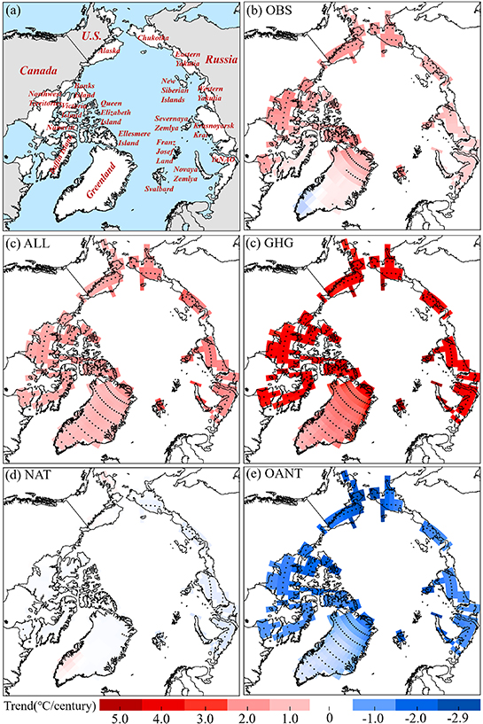
Figure 2. Spatial patterns of the observed and simulated change trends of land surface air temperatures from 1914 to 2015. (a) A map identifying the terrestrial regions of the Arctic; (b) CRU observations (OBS); (c)–(e) ensemble-weighted averages of 9 CMIP6 models that account for ALL, GHG, NAT and OANT forcing agents, respectively. The legend colors indicate only (b)–(e), excluding (a). black point in (b)‒(c) indicates grid cells with significant (p < 0.05) change trend.
Download figure:
Standard image High-resolution image3.2. Detection and attribution of Arctic land air temperature changes at time and space scales
Based on the TLSOF, we quantify the contributions of GHGs, NATs and OANT forcing agents to the observed Arctic land surface air temperature changes. The scaling factors, which scale the simulated temperature responses to best reproduce the observed changes, are shown for the individual and multimodel-weighted mean responses with 90% CIs in figure 3(a). The wider CI means greater uncertainty level, while the narrower one indicates lower uncertainty level. It is found that the multimodel-weighted mean temperature responses to GHGs, NATs and OANT forcings are relatively well aligned with the observations, as indicated by the scaling factors of GHGs (β = 0.84), NATs (β = 0.80) and OANT forcings (β = 0.90) (figure 3(a)). However, large discrepancy is observed between the models, and notably, the CanESM5 model fail to detect the GHG, NAT and OANT signals (figure 3(a)). The RCT indicates that the residual variability that remains in the observations after removing the scaled responses is relatively consistent with the IV in the region as simulated in the climate model control simulations.
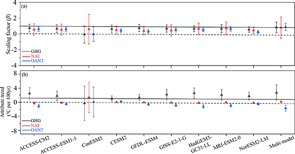
Figure 3. Scaling factors and separate contributions provided by GHG, NAT and OANT forcing agents to historical temperature changes observed from 1915 to 2014 over the Arctic. The scaling factors are based on regressions of the observed annual Arctic mean air temperature anomalies onto the simulated responses to GHG, NAT and OANT forcings. 5%–95% confidence intervals (CI) are represented by bars (segments denote the lower and upper bounds of a CI), and the best estimates are indicated by triangles. A scaling factor with a value larger than zero indicates a detectable temperature response to the corresponding forcing. The solid horizontal line in (b) indicates the observed temperature trend (in °C per 100 years) for Arctic land areas.
Download figure:
Standard image High-resolution imageThe warming trends over 1915–2014 that are attributable to GHGs, NATs and OANT forcings are illustrated in figure 3(b). According to the multimodel-weighted mean, the GHG forcings alone have led to a warming of 2.72 °C (CI: 1.42 °C–4.03 °C) from 1915 to 2014, 1.68 °C (CI: 1.28 °C–2.18 °C) of which was offset by the cooling effects induced by OANT forcings. Compared to the findings of Najafi et al (2015), our calculations, which remove the influences of model drift when calculating internal climate variability, result in smaller GHG and OANT forcing effects. In addition, NAT forcings may have also contributed to 0.12 °C (CI: 0 °C–0.25 °C) of warming over the Arctic. By accounting for all forcing agents, a net warming effect (1.16 °C) close to the observed warming of 1.12 °C is obtained for the study period. The results derived from the best estimates indicate that the OANT forcing has offset 61.8% of Arctic land warming induced by GHG emissions between 1915 and 2014. To assess the robustness of our findings, we repeat our analysis with two additional observational datasets: DGLT and GISS. As shown in supplementary figure 5, the results obtained by using the DGLT and GISS datasets are very consistent with those obtained from the CRU dataset.
The flowchart of the detection and attribution of Arctic land surface air temperature changes at the spatial scale is presented in supplementary figure 6. We also examine the spatial patterns of IV based on the average of 48 individual models to reduce the influence of IV (supplementary figure 7). On the basis of the multimodel-weighted mean, the spatial patterns of the scaling factor and attributable trend are illustrated in figures 4 and 5, respectively. Figure 4 shows that the effects of GHGs, NATs and OANT forcings can be detected in most Arctic land areas. Overall, the multimodel mean temperature responses to GHG forcings are robustly detected (β close to 1) over the Arctic, except for Baffin Island and southern Greenland (figure 4(b)). In contrast, the NAT and OANT responses are overestimated in most regions of Arctic North America (e.g. Alaska, Northwest Territories and Nunavut), but underestimated in the Krasnoyarsk Krai of Russia (figures 4(e) and (h)). Above results indicate that the estimates of the responses to external forcing show large spatial heterogeneity, which is possibly related to the spatial difference in IV over the Arctic (supplementary figure 7)
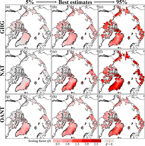
Figure 4. Spatial patterns of the scaling factors by which the simulated Arctic land temperature responds to GHG (a)–(c), NAT (d)–(f) and OANT (g)–(i) forcing agents based on the multimodel-weighted mean. The 5% threshold results, best estimates and 95% threshold results are shown in the first, second and third columns, respectively.
Download figure:
Standard image High-resolution image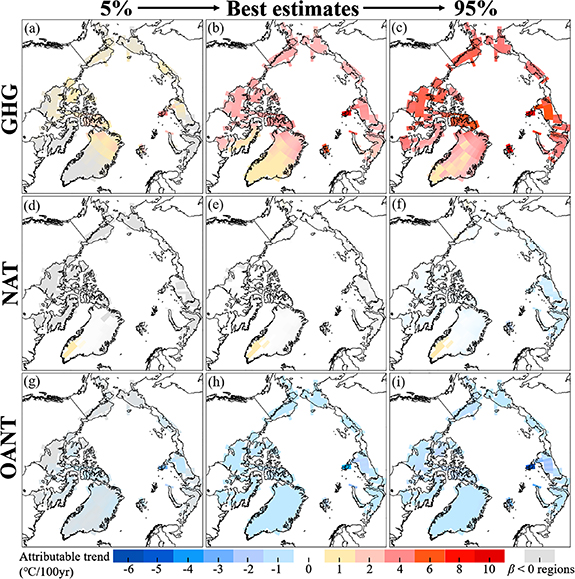
Figure 5. Spatial patterns of the Arctic warming trends that are attributable to GHG (a)–(c), NAT (d)–(f) and OANT (g)–(i) forcing agents based on the multimodel-weighted mean. The 5% threshold results, best estimates and 95% threshold results are shown in the first, second and third columns, respectively.
Download figure:
Standard image High-resolution imageFigure 5 shows the spatial distributions of the warming trends that are attributable to GHGs, NATs and OANT forcing agents. According to the best estimates, a large spatial difference is found regarding the GHG-induced warming trend across the Arctic. The results suggest that GHGs alone have warmed the Arctic by 1 °C–6 °C across the Arctic over the past century, especially in the regions of Ellesmere Island, Severnaya Zemlya, Svalbard and Krasnoyarsk Krai (figure 5(b)). The trend attributable to NAT forcings is close to zero over the whole Arctic, which is consistent with the weak long-term trends of solar and volcanic forcings over this period (figure 5(e)). The cooling effects of OANT forcings reach 1 °C–2 °C in most Arctic land areas except for Severnaya Zemlya (figure 5(h)). Similar spatial patterns are revealed for the temperature responses to GHGs, NATs and OANT forcings based on the DGLT and GISS observations (supplementary figure 8–11), suggesting the robustness of our findings.
3.3. Dynamic evolution of the response signals and attributable trends
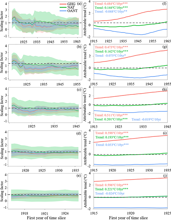
To explore the temporal evolution dynamics of the response signals and attributable trends over the Arctic, the scaling factors and attributable trends are estimated by using moving windows with five different lengths (figure 6). The results indicate that the adoption of a longer time slice leads to smaller IVs (supplementary figure 12). In this section, the average IVs of 48 climate models are used to adjust the observed and simulated temperatures to eliminate the influence of IV on the attribution results. Like previous studies using a large ensemble of climate models to estimate the IV (Najafi et al 2015, Mueller et al 2018), we use all 48 models to account for the uncertainty of IV estimation instead of the nine models. After conducting a variance analysis, nonsignificant (p > 0.05) differences are observed among the IVs within different time slices, with IVs ranging from 0.0026 to 0.0037 °C/year (supplementary figure 13).
Figure 6. Temporal dynamics of the scaling factors (GHGs, NATs and OANT forcings) and the corresponding attributable trends with different lengths of time. (a)–(e) The temporal changes in the scaling factors based on 50-year (a), 60-year (b), 70-year (c), 80-year (d) and 90-year (e) time windows. (f)–(j) The temporal changes in the attributable trends (only for the best scaling factor estimates) based on 50 year (f), 60 year (g), 70 year (h), 80 year (i) and 90 year (j) time windows. The trends in (f)–(j) indicate the change trends of the attributable trends. *, **, and *** indicate statistical significance at the 5%, 1% and 0.1% levels, respectively. The shaded areas represent the 5th and 95th percentiles of the synthetic distribution.
Download figure:
Standard image High-resolution image
Overall, smaller fluctuations in the GHG, NAT and OANT scaling factors are observed for longer time windows (figures 6(a)–(e)). The multimodel GHG, NAT and OANT responses are commonly underestimated (β> 1) between 1915 and the 1960s (figure 6(a)). For the period between the 1920s and 2014, the GHG and OANT signals are overestimated (β < 1) at all slice sizes (figures 6(a)–(e)). In addition, NAT scaling factors from above 1 to below 1 are observed for all window sizes except for 90 years (figures 6(a)–(e)). The strengths of the GHG and OANT signals have increased since the 1930s, with a scaling factor gradually approaching one (figures 6(a)–(e)).
The trends attributed to the GHGs, NATs and OANT forcings when using moving windows with different lengths are presented in figures 6(f)–(j). Due to the large uncertainties of the scaling factors, the best estimates of the attributable trends are used for analysis. For GHG-induced warming, the attributable trends significantly (p < 0.001) increase over time for all window sizes (figures 6(f)–(j)). The effect of OANT forcings is sensitive to the length of the utilized time slice, suggesting great differences in the amounts of aerosol emissions in different periods which could highly impact the relative contribution of each forcing component (figures 6(f)–(j)). The geographical distribution of anthropogenic aerosol emissions exhibited a shift from the western hemisphere to the eastern hemisphere around late 1970s. This evolution of aerosol forcing distribution is expected to have an impact on the Arctic air temperature trend and its spatial pattern. Notably, the sign of the NAT forcing effect has changed from cooling to warming, probably due to the reduction in volcanic activity toward the end of the study period (figures 6(f)–(j)). The revealed temporal evolution patterns based on the DGLT and GISS datasets are basically consistent with those obtained from the CRU dataset (supplementary figures 14 and 15).
4. Discussions
Our results demonstrate that changes in GHGs, aerosols and other anthropogenic forcings have greatly contributed to Arctic temperature changes during the past century. Particularly, 61.8% of the Arctic warming rate is offset by the cooling effect of OANT forcing agents, which are dominated by aerosols. This contrasts with the global-scale analysis, which indicates that only 5% of GHG-induced warming was offset by OANT forcings from 1901 to 2010 (Jones et al 2013). Quinn et al (2008) indicated that the directions, magnitudes and mechanisms of Arctic aerosol forcings are highly dependent on the interactions between long-range transport seasonality, incoming radiation, and the melting and deposition of snow/ice, which can exert a large influence on the Arctic climate (Shindell and Faluvegi 2009). In addition, our study suggests that the influence of NATs on Arctic temperature, which is mainly due to volcanic activity, is detectable and has contributed a small amount of Arctic warming.
Our results also indicate that the warming effects induced by GHG forcings have been higher in Ellesmere Island, Severnaya Zemlya, Svalbard and Krasnoyarsk Krai, which may be associated with the different types of land covers across the Arctic. Indeed, our study indicates larger warming trends in High Arctic regions, where the main types of land cover are barren land and mountains with low plant cover (below 5%) (supplementary figure 16). Besides, greater effects by OANT forcings are generally found in areas with more intensive human activities, probably because anthropogenic sources (e.g. industrial and transportation activities) are large contributors to Arctic air pollution transported from lower latitudes. Further analysis indicates that the GHGs, NATs and OANT forcings were smaller before the 1960s, based on 50 year and 60 year time slices. However, the multimodel-weighted GHG and OANT responses are robustly detected for the recent periods (e.g. the 1960s–2014). The findings of dynamic evolution analysis implies that attribution of Arctic climate change should use as long period of simulations as possible to reduce the impact of IV and obtain more robust results.
To better interpret the findings of our study, however, it is important to acknowledge the inherent uncertainties and limitations. First, although two additional sets of observations are used to evaluate the robustness of our findings, the number of weather stations included in the production processes of CRU/DGLT/GISS remain relatively sparse in the Arctic, thus introducing uncertainty in the temperature estimations. Therefore, further expansion of ground observation stations to obtain more reliable observation data is critical to conduct the attribution study over the Arctic. Second, we spatially attribute Arctic temperature changes to GHGs, NATs and OANT forcings based on CMIP6 climate models. However, the coarse natures of climate models (∼100–250 km horizontal resolutions) would inevitably lead to uncertainty in topography, land cover, and snow/glacier distribution representations, all of which are difficult to resolve in the response signals and attributable trends. In the future, using downscaled or regional climate models may provide new insights for the detection and attribution of Arctic climate change especially at the local scale. Third, because the CMIP6 climate models only account for well-mixed greenhouse gas changes, we cannot identify the separate contributions of individual GHGs (such as CO2, CH4, N2O, and water vapor) to Arctic warming. Hence, additional experiments considering more forcing scenarios would be helpful for enhancing our understandings of the impact of different greenhouse gas agents on Arctic temperature, which has great implications for targeted adaptation and mitigation polices. Fourth, we assign unequal weights to CMIP6 models for attribution of Arctic temperature changes. However, our weighting approach depends on the variable of interest, and it is possible that the models which are good in reproducing observed temperature are poor in terms of other climate variables.
5. Conclusions
In this study, we have investigated the spatial heterogeneity and temporal evolution of the separate contributions of GHGs, NATs and OANT to Arctic land surface air temperatures based on the latest CMIP6 data, using a more robust detection and attribution method. Our results show that GHGs alone have warmed the Arctic by 2.72 °C/century, 61.8% of which has been offset by OANT agents. Compared to previous studies (e.g. Najafi et al 2015), we obtain a smaller magnitude of GHG and OANT forcing effects after removing the influences of model drift. Importantly, the combined effects and relative contributions of GHG, NAT and OANT forcing have changed over time, with GHGs showing the strongest effects after the 1970s and OANT agents exerting increasing influence from 1915 to 2000. Spatially, GHG-induced warming has dominated the areas of Ellesmere Island, Severnaya Zemlya and Svalbard (above 4 °C/century), while OANT agents have exerted the greatest cooling influences in the areas over Krasnoyarsk Krai and Severnaya Zemlya (above −2 °C/century). The NAT effects have been relatively minor but nonnegligible in certain periods and regions, probably due to the reduced volcanic influences. This study highlights the heterogeneously distributed and temporal varying effects of external forcings on Arctic temperature changes during the past century.
Acknowledgments
This research is supported by the National Key Research and Development Program of China (No. 2020YFA0608502), the Special Funds for Creative Research (No. 2022C61540) and the National Natural Science Foundation of China (No. 42077420).
Data availability statement
The data that support the findings of this study are available upon reasonable request from the authors. Data will be available from 01 August 2022.
Supplementary data (6.6 MB PDF)