

Abstract
Climate actions have focused on CO2 mitigation and only some studies of China consider non-CO2 greenhouse gases (GHGs), which account for nearly 18% of gross GHG emissions. The economy-wide impact of mitigation covering CO2 and non-CO2 GHGs in China, has not been comprehensively studied and we develop a multi-sector dynamic model to compare the impact of CO2-only mitigation with a multi-GHG mitigation policy that also price non-CO2 GHGs. We find that the multi-GHG approach significantly reduces the marginal abatement cost and economic loss to reach the same level of GHG emissions (measures as 100 year global warming potential) compared to a CO2-only scenario. By 2060, multi-gas mitigation can reduce the tax rate by 15.44% and improve real gross domestic product (GDP) by 0.41%. The aggregate gain brought by multi-GHG mitigation are robust to various pathways and but vary across periods and sectors.
Export citation and abstract BibTeX RIS

Original content from this work may be used under the terms of the Creative Commons Attribution 4.0 license. Any further distribution of this work must maintain attribution to the author(s) and the title of the work, journal citation and DOI.
1. Introduction
In the Paris agreement reached at the 21st Conference of the Parties (COP-21) of the United Nations Framework Convention on Climate Change in 2015, nations made their 'nationally determined contributions (NDCs),' and China set a goal to cut CO2 emissions per unit of GDP by 60%–65% by 2030, compared to 2005 levels. The actual carbon intensity has fallen another 22% between 2014 and 2019, just before the Covid19 pandemic hit. In 2020 the government announced very ambitious targets to peak absolute carbon emissions before 2030 and to achieve carbon neutrality by 2060. This is the most significant national contribution to the global goal to limit climate impacts given that the NDCs of the most developed countries is to reach carbon neutrality by 2050. These commitments and announced actions mainly refer to CO2 governance, less attention was paid to non-CO2 greenhouse gases (GHGs) 4 , which account for nearly 18% of gross GHG emissions [1]. It was only during COP26 in 2021 that methane pledges were made. As many authors have pointed out, if policymakers ignore the options to abate non-CO2 GHGs they would likely not be using the optimal approach [2–4]. To combat climate change cost-effectively, it is crucial to consider multi-GHG mitigation and to evaluate the corresponding benefits and costs.
There are many studies analyzing China's climate actions where they include two aspects: pathway simulation and policy evaluation. Some consider the pathways necessary to achieve specific climate goals [5–9]. For instance, He et al [6] estimated the required reduction of fossil energy consumption and CO2 emissions under the 2 °C and 1.5 °C scenarios. Zhang et al [7] conducted a comprehensive assessment of the pathways and policies toward carbon neutrality by 2060. Other papers analyze climate policies, such as the emission trading system (ETS) [10–13], or carbon taxes [14–16]. However, these focus mainly on cost-effective CO2 mitigation, with only a few on non-CO2 GHG reduction, especially from the perspective of economic instruments and their impact.
Existing studies on non-CO2 GHGs are more about projecting their pathways and assessing their abatement potential based on bottom-up methods. Lin et al [17] used a bottom-up end-use modeling approach to make a detailed projection of non-CO2 GHG emission trajectories by 2050 while Duan et al [18] conducted a multi-model study and pointed out the crucial role of curbing non-CO2 GHGs to meet the 1.5 °C warming limit. However, there are very few papers about how to reduce non-CO2 GHGs through economic instruments and the economy-wide effects of such market policies. Existing research primarily study the situation before 2050 or earlier [1, 19–21]. In the context of the ambitious 2060 carbon neutrality goal, stabilizing climate change with lower costs necessitates a comprehensive economic analysis of multi-gas mitigation, covering both CO2 and non-CO2 GHGs.
To assess the economy-wide effects of multi-GHG mitigation, we employ a multi-sector dynamic general equilibrium model combined with detailed non-CO2 GHG inventories with a detailed set of technologies for the power sector. While partial equilibrium bottom-up models provide fine-grained detail of production technologies [22–25] and integrated assessment models provide linkages with climate variables [26–28], the top-down computable general equilibrium (CGE) model can characterize the inter-industry general equilibrium effects of policies. For example, the model traces the impact of a carbon price on coal and electricity prices, how these affect the cost of making steel, which in turn, affects the cost of building power plants. Our model of China has 33 sectors with seven electricity generation technologies so that we can capture the substitution of renewable capital for fossil fuel inputs more precisely compared to models with an aggregate electricity sector. We simulate a business-as-usual (BAU) scenario and two policy scenarios—CO2-only mitigation and multi-GHG mitigation.
We find that a CO2-only policy can generate a positive, but limited, spillover effect on reducing non-CO2 GHG emissions. When we consider a multi-gas policy that reaches the same level of total GHG-equivalent reductions as the CO2-only case, the abatement costs and economic losses are considerably lower. The benefits of the multi-GHG policy are small in the early stages of modest reductions in GHG emissions but magnify with greater cuts over time. By 2060, multi-gas mitigation will reduce the carbon tax rate by 15.44% and reduce GDP losses by 0.41%. Moreover, our findings are robust to several emission pathways and technology conditions.
2. Methods
2.1. Economic-environmental model of China
We developed an economic-energy CGE model to simulate the effects of climate policies on growth and emissions in China. The model incorporates 33 sectors and has a dynamic recursive structure with an exogenous savings rate that determines investment. Economic growth is driven by investment, population growth, total factor productivity (TFP) growth, and changes in the quality of labor. The model comprises five main actors: producers, households, government, capital owners, and foreigners. A social accounting matrix for 2014 based on the benchmark 2012 input-output table is the key input into the model. This section summarizes the key features of the model, further details are in the appendix, and a detailed description is given in a separate appendix of Cao et al [14].
The 33 sectors identified in the model are given in table A1, with output, value-added, and number of workers in the base year 2014. Each sector produces its output using a constant returns to scale technology, and constant elasticity of substitution (CES) functions taken from the Global Trade Analysis Project (GTAP) model (version 7) 5 . The production function and nested structure of production is shown in appendix figure A1. TFP growth is set exogenously; we have not included an endogenous version where TFP depends on input prices or research and development spending.
The realization of carbon neutrality would require a deep transformation of the power sector and we disaggregate the electricity sector into seven generation technologies to characterize the structural change from coal power to renewables. The structure of the electricity sector is shown in appendix figure A2. At the top tier, electricity output is an aggregate of transmission & distribution and electricity generation, in the second tier generation consists of base load sources (coal, gas, nuclear, hydro, coal with CCS, gas with CCS, and others) and intermittent renewables (wind and solar). To recognize the likelihood that technologies to extract carbon from the atmosphere, or from industrial processes, will be necessary to reach the ambitious neutrality goals, we allow a backstop technology that gradually raises the rate of carbon extraction.
In the transportation sector and home-heating we do not model distinct technologies such as electric vehicles or electric heating. In such sectors, our industry production functions represent some substitution between fuels and electricity, and between total energy and capital. The substitution of electric vehicles for combustion engines is thus not well represented and our functions may understate the degree of electrification.
For households, private consumption is driven by an aggregate demand function that is derived by aggregating over different household types. Each household derives utility from the consumption of commodities, is assumed to supply labor inelastically, and owns a share of the capital stock. Total consumption expenditures are allocated to the 33 commodities identified in the model. The demand function is estimated over household consumption survey data as described in Hu et al [29].
The government imposes taxes, purchases commodities, pays for carbon sequestration, and redistributes resources. Public revenue comes from direct taxes on capital and labor, value-added taxes, indirect taxes on output, consumption taxes, tariffs on imports, externality taxes, and other non-tax fees. Trade flows are modeled using the standard Armington method used in most single-country models. Current account and government deficits are set exogenously.
2.2. GHG accounting
We adopt a top-down approach to account for CO2 emissions where combustion emissions are given by the national quantity of fuel consumed, multiplied by the energy content coefficient and the CO2 intensity per unit energy. For non-combustion sources of CO2, we only consider those from cement production processes which are given by an emission factor multiplied by the cement component of the output of the building materials industry.
Non-CO2 GHGs emissions are counted using a bottom-up method. The Non-CO2 GHG inventories are based on The People's Republic of China First Biennial Update Report on Climate Change [30]. We disaggregated non-CO2 GHGs into various sectors according to the sources and GHG types, and calculated emission coefficients based on total production and emissions. Since the various GHGs have different warming potentials and lifetimes, we convert non-CO2 GHGs to CO2-equivalents at 100 year global warming potential (GWP) 6 according to the IPCC Second Assessment Report [31]. We also consider technological advances related to non-CO2 GHG mitigation by calibrating the non-CO2 GHG emission pathway according to Lin et al [17], which employs a comprehensive bottom-up end-use modeling approach. Our estimated inventories for 2014 are given in appendix table A5.
2.3. Simulation scenarios
We develop one baseline scenario and two climate policy scenarios for GHG mitigation. We also consider the impact of an exogenous improvement in technologies that reduce the output of non-CO2 gases. For the baseline BAU case, we incorporate the 'Current Policies' projections from the World Energy Outlook 2018 (IEA 2018) that incorporates policies that were announced up to that point. We calibrate a gradual change in energy use parameters in the production and consumption functions over 2014–2040 to reach the projected national use of coal, oil, gas and renewable electricity.
In the policy scenarios, a GHG price is imposed such that the CO2 emission pathways reach the carbon neutrality target by 2060. Carbon capture and sequestration is likely to play a key role in the future, however, there is a great deal of uncertainty about the costs of such technologies. Here we take a simple approach and assume that negative carbon technologies will be available beginning in 2031 and costs will fall over time. We assume an exogenous path of carbon sequestration that rises from zero in 2030 to about 6000 million tons of CO2 by 2060 (compared to the total 22 600 in the base case). We also assume that there are no environmental costs in sequestering carbon. The endogenous GHG price serves as a proxy for all climate policies and reflects the economy-wide marginal cost of abatement, that is, it reflects the policy efforts needed to achieve carbon neutrality. We implement the carbon price as a simple upstream carbon tax on fossil fuels including imported fuels, this avoids the complexity of ETSs.
- (a)Baseline scenario. The base case growth path is determined by the exogenous variables of labor force, demographic change, saving rates and TFP growth. Cao et al [14] give a detailed description of the settings of the base case. Figure 1 presents the simulation results of the main economic variables from 2014 to 2060 in the baseline scenario: GDP growth falls from 7.4% per year in the beginning to 2.2% by 2060 due to the falling labor force and investment; the consumption share of GDP rises as the investment share falls with the falling saving rate. GDP per capita grows more slowly as the population ages with an expanding retired group. The energy intensity falls steadily with a shift from manufacturing to services and improvements in technology, by 2060 it is 63.7% below the intensity in 2014. The CO2-intensity falls even faster with a shift from coal to other sources of energy.
- The emissions targets set by the government are the timing of the peak and timing of net zero emissions, they do not set a particular path of emissions. In the climate policy scenarios, we set four emission pathways according to these targets, one set by us and three from other studies. In the main '30&60' pathway, carbon emission peaks in 2030 and reaches carbon neutrality by 2060. We emphasize that this target is in terms of CO2 only, not total GHGs. In addition, China's NDC also specified that by 2030, the CO2 emissions per unit of GDP will be 65% of the 2005 level. We present the four pathways to reach these targets in figure 2. Our pathway peaks at 12.0 billion tons from 10.8 in 2014. The emission pathway proposed by Zhang et al [7] is somewhat similar to ours; their emission also peaks around 2030 but at a lower level. We also examine the pathways that China need to meet to contribute to the global goal of limiting warming to 1.5 °C in studies by BCG [32] and Duan et al [18]. To achieve the 1.5 °C target, CO2 emissions peak immediately in 2022 and decline continuously till 2060. The peak value of CO2 emission by Duan et al [18] is higher than BCG, and the slope is correspondingly steeper.
- (b)CO2-only mitigation scenario. The carbon emission pathways are achieved through taxing CO2 emissions. We impose an upstream tax on fossil fuels based on the carbon content, which includes domestic producers of fossil fuels and the imports of all fuels. We implement a revenue-neutral policy by recycling the carbon tax revenue as a cut to all other tax rates. The tax cut is chosen such that real aggregate government consumption and the deficit is the same as the base case for each period. Decarbonizing the electricity sector alone cannot lead to carbon neutrality since other sectors consume fossil energy, such as transportation, manufacturing, and households. Electricity, however, is the most important source of emissions and the path of power generation is a key determinant of the path to carbon neutrality. One may choose a path with higher electricity prices and lower electricity use, but we have chosen a path where electricity consumption is equal to the base case path by introducing a renewable energy subsidy to keep electricity prices from rising.
- (c)Multi-GHG mitigation scenario. In this scenario we put a price on all the identified GHG emissions, including CO2, methane and the gases listed in table A4. One may implement a non-CO2 GHG price either by adding new taxes to the existing environmental tax system or through the Certified Emission Reduction Project in the ETS. For simplicity, and to ensure comparability with the CO2-only policy, we impose a unified, endogenous GHG price that is set so that the total GHG emissions (in CO2-equivalent units) of the two policy scenarios are the same. This means that the multi-gas mitigation path has higher CO2 emissions but lower non-CO2 GHG emissions. The multi-GHG mitigation policy is also revenue-neutral, and the total quantity of electricity generation remains the same as in the CO2-only case. The summary settings of the baseline, CO2-only and multi-GHGs mitigation scenarios are shown in table 1.
- (d)Technology shocks and alternative GWPs. We briefly consider the impact of exogenous changes in technologies that reduce the non-CO2 emission coefficients to illustrate the magnitudes involved. Considering the divergent stock and flow effect of each GHGs, we conduct a sensitivity test using an alternative GWP with a 20 Year horizon, shown in appendix table A2. This emphasizes the short-term radiative effects of some of these gases.

Figure 1. Economic indicators for baseline scenarios.
Download figure:
Standard image High-resolution image
Figure 2. CO2 emission pathways.
Download figure:
Standard image High-resolution imageTable 1. Simulation scenarios.
| Scenario | Baseline | CO2-only | Multi-GHG |
|---|---|---|---|
| Government consumption | BAU | BAU | BAU |
| Electricity generation | BAU | BAU | BAU |
| Revenue-neutral | Cut other tax | Cut other tax | Cut other tax |
| Negative emission technology | No | CO2 | CO2 |
| Emission pathway | BAU | CO2 emission == CO2 pathways | Total e-GHGs emission == CO2-Only case |
| Tax object | No | CO2 | CO2 + non-CO2 GHGs |
Notes: 'BAU' represents the results of business-as-usual scenario without climate policies.
3. Results
3.1. Baseline scenario
We have noted that the base case GDP grows at a fast rate in the beginning and then decelerates rapidly with the fall in the labor force. Recall also that we use the 'current policy' projections from the International Energy Agency. The simulated paths for electricity generation and GHG emissions in the baseline scenario are given in figure 3. The demand for electricity rises, but a rate slower than GDP growth, and the generation structure undergoing continuous transformation towards less coal and more renewables. As shown in figure 3(a), coal power generation remains almost unchanged from 2014 to 2060, while clean energy from wind, solar, and nuclear power rises rapidly.
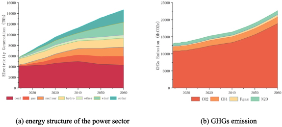
Figure 3. Baseline scenario simulation results.
Download figure:
Standard image High-resolution imageAlthough the power sector is changing significantly, carbon emissions from the whole country are not falling and there is an increase in aggregate GHG emissions. As shown in figure 3(b), the growth rate of CO2 and non-CO2 GHG emissions gas emissions remains in the range of 0.4%–1.8%, compared to GDP growth of 2%–7%. Thus, while the emission intensity of GHGs is falling, the absolute amount is still rising. The emission path in the base case is far from the '30–60' decarbonization goal, and stringent climate policies are needed to curb the growth of GHG emissions to reach it.
3.2. CO2-only mitigation scenario
In the CO2-only mitigation scenario, we impose a CO2 tax on fossil fuels and recycle it by cutting pre-existing taxes and providing a subsidy to renewable electricity. For the neutrality target we count just CO2. As noted, we allow technologies that extract CO2 from the atmosphere (or industrial processes); the amount assumed to be reduced is shown by the green dotted line in figure 4(b).

Figure 4. CO2-only mitigation scenario simulation results.
Download figure:
Standard image High-resolution imageWe have four pathways in this scenario and first present results under the main pathway: CO2 emission peaking by 2030 (and reaching 65% of the 2005 carbon intensity) and carbon neutrality by 2060 (not GHG neutrality). The carbon tax reduces GDP immediately and the lower investment cumulates to a net 7.9% loss in 2060 GDP compared to the base case. The carbon price rises over time as shown in figure 5(b) (dark blue squares), while the change in GDP is in figure 5(a). As shown in figure 4(a), the share of fossil fuels dwindles in the power sector, while the proportion of non-fossil energy rises steadily to 100%. Recall that we keep the total MWh output the same as the base case using an endogenous subsidy that keeps the electricity prices from rising much above the base case.
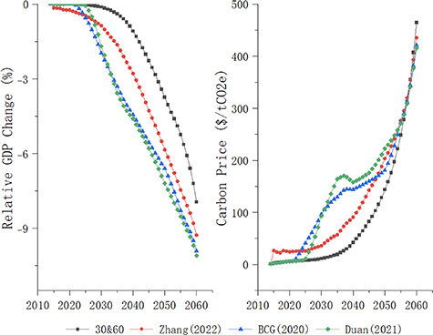
Figure 5. GDP change and carbon price under CO2-only mitigation scenario.
Download figure:
Standard image High-resolution imageThe CO2 tax leads to a significant reduction in fuel use by the rest of the economy, but gross CO2 emissions do not fall to zero. As illustrated in figure 4(b), CO2 emissions in 2060 will be completely offset by negative emissions technologies (about 6 billion tons). That is, of the base case 2060 CO2 emissions of 17 billion tons, the reduction of CO2 production due to the carbon price contributes 68.5%, and the negative emission technology contributes 31.5%. The changes in the economy due to the CO2-only tax also reduces non-CO2 GHG emissions by 13.0% in 2060. Part of the decline in non-CO2 GHG emissions is due to the reduction of fossil energy production since methane leakage from coal mining is an important source. However, the spillover effect of the CO2-only tax on non-CO2 GHG emissions is limited because they come primarily from agriculture, industrial processes, and waste treatment.
We also investigate the impact of the CO2 tax under the three alternative pathways given in figure 2. Figure 5 gives the effect on GDP and the carbon price paths for all four cases. To achieve carbon neutrality by 2060, the marginal abatement cost of carbon emission rises rapidly over time, with corresponding rising losses in GDP. In the main 30&60 emission pathway, the pressure of CO2 reduction is lower in the early stages, and so the carbon price and economic losses are smaller. In later periods, the pressure of emission reduction surges and the carbon price and economic losses escalate. Compared with the baseline scenario, real GDP in 2060 will fall by 7.9%, and the carbon price will reach more than 465 $/tCO2e (in 2014 US$).
For the pathway proposed by Zhang et al [7] the effects are similar: CO2 emission peaks in 2030 but at a lower level. The pattern of GDP and carbon price under this path is similar to the main pathway. Due to the lower peak value, the GDP loss here is higher: 9.28% compared with 7.9% in the main pathway. Under the pathways of BCG [32] and Duan et al [18], however, the carbon price climbs quickly in the early stages, and the economic losses are bigger than those in the'30&60' pathway. Compared to 2014, the GDP in 2060 is lower by 9.90% and 10.10%, respectively. The results suggest that such a rapid decarbonization in the early years is very costly; this is during a period when China has not yet reached a high-income status according to the World Bank definitions.
We should note that the simulated GDP losses depend on the structure of the model and parameters used. Keppo et al [33] point out that carbon pricing in most models does not target technology transition and does not capture how policies may affect technology innovation. Our model also does not have a role for R&D spending or endogenous TFP. Allowing such effects could change the estimated GDP loss.
3.3. Multi-GHG mitigation scenario
In the Multi-GHG mitigation scenario we tax non-CO2 GHGs at the same tax rate as CO2 emissions. For comparability, the tax is set such that total GHG emissions (in CO2-equivalent units at 100 year GWP) and electricity consumption in the two scenarios are the same each year. In another words, the impact on global warming is equivalent between these two scenarios under the assumption of a 100 year GWP time scale (we also report a test using a 20 year GWP assumption).
Figure 6 and appendix table A7 summarizes the relative changes in key economic and environmental variables due to the multi-GHG tax policy (compared to the CO2-only policy), for each of the four pathways. Table A7 panel A shows the near-term results in 2030. For GDP and its major components, there is very little difference between the two policies. The multi-GHG carbon price is slightly lower by 0.72%–1.01% for the four pathways. As for environmental indicators, the multi-GHG tax has slightly higher CO2 emissions (+0.01% in 30&60) while reducing non-CO2 GHG emissions, especially CH4 and N2O (−0.05% in 30&60). Overall, in the early stages, there is little difference in environmental and economic impacts between multi-GHG tax and CO2-only tax.
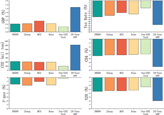
Figure 6. Relative changes in critical economic and environmental variables.
Download figure:
Standard image High-resolution imageBy 2060, however, the difference between the two taxes is substantial. As shown in figure 6, spreading the burden over more gases, i.e. over more emitters, reduces the carbon price by 15.4% (from 465 $/tCO2 to 393 $/tCO2) in 30&60 compared to the CO2-only policy and GDP is higher by 0.41% (higher in levels, not in growth rate). This is small, but non-trivial, compared to the overall 7.9% fall in GDP in the CO2-only case. The small effect is comparable to the small change in carbon prices. Moreover, the improvement of multi-GHGs policy is systematically positive for all four pathways. Coal consumption is higher by 8.6%, and oil by 0.7%, in the multi-GHG case (30&60 pathway) and total CO2 emissions is higher by 116 million tons. This is offset by non-CO2 GHG emissions being 3.6% lower.
Along the CO2-mitigation only path, negative emission technologies share a partial burden of GHG reduction, however, the marginal reduction costs still rise dramatically. By 2060, the tax rate reaches around 420 $/tCO2e and GDP loss is up to 10% in the BCG and Duan pathways. This results in net zero CO2 emissions and a 13% reduction in non-CO2 GHG emissions, giving an 85.6% reduction in total GHG.
3.4. Role of technology change and GWP assumptions
In a sensitivity check we consider the impact of technological advances that lower the non-CO2 GHG emission coefficients such as different livestock feed and leakage control. Lin et al [17] give projected trajectories of non-CO2 GHG emissions for China and we simulated a scenario where the GHG emission coefficients fall like their baseline pathway, as shown in appendix table A6. In column 'Non-CO2 Tech' of table A7 we give the impacts on economic and environmental variables of this technology change.
The change in technology results in a significant cutback in non-CO2 GHG emissions, even under the CO2-only Mitigation Scenario; −48% in 2060 compared to the −13% in the fixed-technology cases. Since these technological advances reduce the opportunity to cut non-CO2 emissions, they weaken the ability of multi-GHG taxes in reducing abatement costs and improving economic growth compared to the CO2-only tax case. Here the multi-GHG carbon price in 2060 is only 6.9% lower than the CO2-only policy, compared to a 15.4% reduction in the fixed-technology case. Nonetheless, the multi-GHG tax in this technology shock case still improves GDP by 0.27% in 2060 compared to the 0.41% improvement in the fixed-technology case.
So far, we calculated the GWP of GHGs using the 100 year horizon. Since the lifetimes of some gases are short (about a decade for methane) it may be argued that different time horizons may be more appropriate. To check how our results depend on this assumption, we recalculated the CO2-equivalents using a 20 year horizon. We then simulate the two policy scenarios with the new coefficients and the impact is given in the GWP 20 year column in table A7. The carbon price in 2060 is lower than in the GWP100 case (−23% vs. −15%), leading to higher CO2 emissions but a bigger cut in non-CO2 emissions. The lower carbon price gives a bigger recovery to GDP from the CO2-tax case. This shows that the GWP assumption is important for the exact outcomes, but the direction is the same.
Different emission pathways and technology scenarios all point to the same conclusion that multi-GHG tax can effectively alleviate the pressure of CO2 emission reduction in the later stages of reaching carbon neutrality. Taxing all GHGs reduces the need for reducing CO2 and thus lessens the mitigation costs significantly.
3.5. Effects of policies at the sector level
Next, we examine the impact of climate policies across the 33 sectors in 2060. In figure 7 the blue bars represent the impact of CO2-only tax on industry output relative to the baseline scenario while the orange bars represent the changes in multi-GHG scenario compared to the CO2-only Scenario.

Figure 7. Relative change in output by sector.
Download figure:
Standard image High-resolution imageCompared with the baseline scenario, the CO2 tax leads to a decline in the output of most sectors. Three sectors are directly affected by the CO2 tax and their output falls the most: coal mining (−74.7%), oil mining (−26.4%), and natural gas mining (−60.6%). The higher price of fossil energy due to the tax raises costs in energy-intensive downstream industries, such as petroleum processing, primary metals, metal products, gas utilities, and transportation services. This leads them to charge higher prices and their output falls by much more compared to the less energy-intensive industries. The carbon tax and renewable subsidy push the transformation of the power sector, gradually reducing fossil fuel use to zero. To recall, the subsidies were chosen to maintain power output at base case levels to allow a simple comparison. If there were no subsidies, the electricity prices would be higher and power consumption would be discouraged. Our revenue neutrality condition maintains the government share of final demand and avoids a source of difference for welfare comparisons across the three scenarios. The assumption of free movement of labor and new capital means that factors moved out of the shrinking energy-intensive sectors to the other sectors, such as agriculture and electrical machinery.
The results in appendix table A7 show that taxing all GHG emissions requires a lower tax rate to reduce the GHG emissions by the same amount relative to the CO2-only tax. The lower carbon prices reduce the impact on the fossil energy intensive sectors, as shown in the orange bars in figure 7, the output of refining, primary metals, and building materials are slightly higher. We should note that the multi-GHG tax restricts the output of sectors with low CO2 but high non-CO2 GHG emission intensity, such as electrical machinery, water utilities, and agriculture. There is a very small change in agriculture output because there is an opposing effect, in the CO2-tax only case, agriculture output is higher than in the base case because of a switch in expenditures from energy-intensive goods to agriculture and services. The non-CO2 GHG tax on emissions from agricultural activity reduces this switch and offset some of the effect of the tax on non-CO2 emissions from agriculture.
4. Conclusion
This study compares the impact of two different climate policies aimed at reaching the carbon-neutral targets. A policy that taxes only carbon emissions would induce profound structural changes in the electricity sector and significantly reduce CO2 emissions and encourage sequestration. It can generate a positive, but limited, spillover effect on reducing non-CO2 GHG emissions. To curb CO2 emission to zero by 2060, we estimate that very high CO2 prices are needed; about 465 $/tCO2 by 2060, which is consistent with other studies [7, 18, 34]. This is the case even after assuming the use of negative carbon technologies. This high price of CO2 lowers real GDP by 8%–10% in 2060, relative to the baseline scenario.
We find that a multi-GHG mitigation policy can reduce abatement costs and economic losses while achieving the same climate impact. In the early stages, the impacts of a CO2-only or multi-gas policy are similar. As mitigation costs spike in the later periods, however, the benefits of multi-GHG mitigation rise significantly. Compared with CO2 only mitigation policies, multi-gas mitigation will reduce the tax rate by 15.44% and reduce GDP losses by 0.41% in 2060. It also mitigates the negative impact of CO2-only tax on carbon-intensive sectors, except for sectors with high non-CO2 GHG emissions such as electrical machinery, water utilities, and agriculture.
Currently, specific binding targets are still missing in China's NDCs for non-CO2 GHGs reduction. Our simulations show that it is important to explore the co-control of CO2 and non-CO2 GHGs to combat climate change in a cost-effective manner.
There are limitations of this type of simulation analysis. In our model, technological advances are exogenously given, which may underestimate the gains of multi-GHG mitigation when the policy may induce research efforts in speeding up the reduction of non-CO2 GHG emissions. In addition, our model does not consider the institutional costs of implementing climate policies, leading to an underestimate of total economic losses. This may be especially important for non-CO2 GHGs which have more dispersed sources. It is hard to levy an upstream tax like a CO2 tax with higher costs of monitoring and regulation. We have implemented a very simple characterization of the cost of negative carbon technologies; when better projections of future costs are available, they will be crucial in determining the actual cost of mitigation. Future analysis should consider endogenous technology change and institutional costs. We have not included important technologies like power storage or geo-thermal power in our model and will be important to have them in future research.
Acknowledgment
This study is supported by the Research Center for Green Economy and Sustainable Development, and Institute for Global Development, Tsinghua University. Ho is supported by the Harvard Global Institute. We are grateful for the comments and advice of the editor and two referees.
Data availability statement
The data that support the findings of this study are available upon reasonable request from the authors.
Appendix: Model description
The key input into the model is the social accounting matrix (SAM) for 2014. This traces the flow of commodities and payments among the producers, household, government and rest of the world. The SAM is assembled from the 2014 input output table which was derived from the 2012 benchmark IO table 7 . The 33 industries identified in the model are given in table A1 together with their output, value added and number of workers in the base year 2014.
Table A1. Industries in China model, 2014.
| Gross output (bil yuan) | Value added (bil yuan) | Workers (mil) | ||
|---|---|---|---|---|
| 1 | Agriculture | 10 151 | 6388 | 194.348 |
| 2 | Coal mining | 2183 | 928 | 7.752 |
| 3 | Oil mining | 955 | 566 | 0.925 |
| 4 | Natural gas mining | 224 | 112 | 0.182 |
| 5 | Non-energy mining | 1961 | 751 | 4.336 |
| 6 | Food mfg. | 10 743 | 1720 | 12.482 |
| 7 | Textiles | 4341 | 677 | 14.606 |
| 8 | Apparel, leather | 3616 | 659 | 18.429 |
| 9 | Sawmills and furniture | 2362 | 399 | 7.694 |
| 10 | Paper, printing, recording media | 3807 | 708 | 5.901 |
| 11 | Petroleum processing | 4320 | 375 | 0.993 |
| 12 | Chemicals | 14 470 | 2279 | 17.949 |
| 13 | Nonmetal mineral products | 6050 | 1129 | 8.426 |
| 14 | Primary metals | 12 048 | 1734 | 5.687 |
| 15 | Metal products | 4120 | 667 | 7.950 |
| 16 | Machinery | 8478 | 1494 | 11.945 |
| 17 | Transportation equipment | 8266 | 1445 | 6.943 |
| 18 | Electrical machinery | 6305 | 938 | 11.093 |
| 19 | Comm. equip, computer, electronic | 8055 | 1347 | 12.417 |
| 20 | Water utilities | 362 | 146 | 0.750 |
| 21 | Other manufacturing, recycling | 814 | 437 | 6.756 |
| 22 | Electricity, steam | 3778 | 1346 | 3.467 |
| 23 | Gas utilities | 473 | 88 | 0.183 |
| 24 | Construction | 16 709 | 4114 | 61.499 |
| 25 | Transportation svc | 7429 | 2777 | 22.484 |
| 26 | Telecommunications, software and IT | 3321 | 1564 | 4.828 |
| 27 | Wholesale and retail | 8924 | 4679 | 77.399 |
| 28 | Hotels and restaurants | 2714 | 1065 | 24.063 |
| 29 | Finance | 7737 | 4380 | 14.464 |
| 30 | Real estate | 5070 | 3417 | 11.971 |
| 31 | Business services | 8991 | 3075 | 17.499 |
| 32 | Other services | 8613 | 4782 | 131.390 |
| 33 | Public administration | 3934 | 2370 | 45.715 |
The exogenous variables in the model include total population, working age population, saving rates, dividend payout rates, government taxes and deficits, world prices for traded goods, current account deficits, rate of productivity growth, rate of improvement in capital and labor quality, and work force participation. These variables may, of course, be endogenous (i.e. they interact among each other) but we ignore this and specify them independently. Our assumptions for these exogenous drivers are summarized in table A2. Table A3 lists variables which are referred to with some frequency.
Table A2. Parameters of base case growth path.
| Savings rate | Dividend rate | Population | Work force | Labor input (quality adjusted) | Total factor productivity index | |
|---|---|---|---|---|---|---|
| Base year 2010 | 41.2% | 38.9% | 1360 | 938 | 100.0 | 100.0 |
| 2020 | 22.3% | 57.9% | 1440 | 930 | 108.5 | 111.5 |
| 2030 | 17.0% | 63.2% | 1470 | 884 | 108.5 | 122.8 |
| 2040 | 15.3% | 64.9% | 1466 | 838 | 105.9 | 133.9 |
| 2050 | 14.6% | 65.5% | 1434 | 758 | 97.6 | 144.6 |
Table A3. Selected parameters and variables in the economic model.
| Endogenous variables | |
| QIi | total output for sector i |
| VE | primary factor-energy basket |
| M | non-energy intermediate input basket of the 27 non-energy commodities |
| VA | value added consisting of the three primary factors |
| E | energy basket |
| K | capital |
| L | labor |
| T | land |
| Parameters | |
| σ | elasticity of substitution between two inputs of CES function |
| α | the weight for one of the input of CES function |
| g | total factor of productivity |
The assumption that affects the growth rate the most is the household savings rate, st . Our assumption is to have st beginning at the observed 38.9% for 2014 and gradually falling to 30.8% in 2020 and 22.6% in 2030. National private savings is household savings plus the retained earnings of enterprises. The share of retained earnings is assumed to fall, and dividend payouts to rise to reflect the diminishing role of state enterprises in the economy. The dividend rate, i.e. the share not used for retained earnings, was 41.7% in 2014 and we project it to rise to 53% by 2020. It should be pointed out that national savings and investment in the Chinese data includes capital such as roads and other public infrastructure, items that are excluded from the 'gross fixed private investment' item in the National Accounts of most other countries. There is a population projection from UN (2015).
The rate of productivity growth is another factor that has a large effect on the base case growth rate of the economy but has little impact on the difference between cases. To keep the base case as simple as possible we ignore this wide range of observed TFP growth, and in our projections of sector productivity terms we initially set all TFP to the same value and then adjust them to match actual GDP growth rates in the initial years for which we have actual data. The value share parameters of the production functions are set to the values in the 2014 IO table in the first year of the simulation. For future periods we change most of these parameters so that they gradually resemble the shares found in the US input output table for 2007. The exceptions to this are the coal inputs for all the sectors, this is set to converge to a value between current Chinese and US2007 shares 8 . The rate of reduction in energy use is calibrated to the projections in IEA (2016) out to 2040.
We represent the production structure with the cost dual, expressing the output price as a function of input prices and an index of technology. The 3 primary factors and 33 intermediate inputs for each industry are determined by a nested series of CES functions taken from the GTAP model (version 7). The nest structure is given in figure A1 and applies to all industries except electricity which is treated separately below. We use firm-level survey data from the China State Administration of Taxation, Ministry of Finance, to estimate the production functions and elasticities of substitution between inputs. This dataset includes 1824 400 firms with 4946 500 observations from 2007 to 2015. More specifically, there are 220 000 firms in 2007, increasing to 699 900 firms in 2015. A detailed description is given in Cao et al [36].
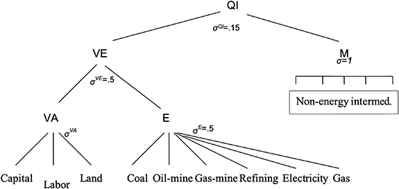
Figure A1. Production structure for each industry except electricity.
Download figure:
Standard image High-resolution imageAt the top tier, output is a function of the primary factor-energy basket (VE) and the non-energy intermediate input basket (M),  . The VE basket is an aggregate of value added (VA) and the energy basket (E). Value added is a function of the three primary factors—capital (K), labor (L) and land (T). The energy aggregate is a CES function of coal, oil mining, gas mining, petroleum refining & coal products, electricity and gas commodities. The materials aggregate (M) is a Cobb–Douglas function of the 27 non-energy commodities.
For the top tier, the production function form is shown in equation (1), where  is the weight for all non-energy inputs into industry j, and
  is the elasticity of substitution between the two inputs.
  is the index of the level of technology where a rising value indicates positive TFP growth and falling output prices,
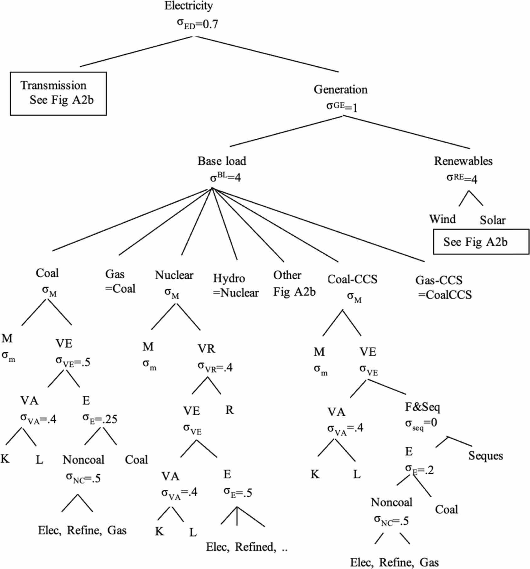
We disaggregate the electricity sector into different generation technologies. The production and input structure of this sector is illustrated in Figure A2; this consists of a nested structure of CES functions. At the top tier, electricity output is an aggregate of transmission & distribution and electricity generation. At the generation node we assume that this consists of base load sources and renewables (intermittent) in a way similar to the C-GEM model (Qi et al 2014). Renewables here consist only of wind and solar which are intermittent sources and often require either parallel storage capacities, or conventional backup. We thus assume that such electricity is imperfectly substitutable with base load sources and specify an elasticity of substitution,  , in a way similar to Qi et al (2014) for our main parameter value of 1.0
9
. All other sources of electricity contribute to the base load aggregate with a high elasticity of substitution,
, in a way similar to Qi et al (2014) for our main parameter value of 1.0
9
. All other sources of electricity contribute to the base load aggregate with a high elasticity of substitution,  = 4
10
. In the base year, these sources include conventional coal, gas, hydro, nuclear and a minor 'other' (oil, biomass, geothermal, etc). In the future years we allow the options of coal with carbon capture and storage (CCS) and gas with CCS. For the intermittent renewable aggregate, we only identify two types in this model: wind and solar (the others are part of the miscellaneous 'other' in the base load tier). We assume that wind and solar are close, but not perfect, substitutes with an elasticity
= 4
10
. In the base year, these sources include conventional coal, gas, hydro, nuclear and a minor 'other' (oil, biomass, geothermal, etc). In the future years we allow the options of coal with carbon capture and storage (CCS) and gas with CCS. For the intermittent renewable aggregate, we only identify two types in this model: wind and solar (the others are part of the miscellaneous 'other' in the base load tier). We assume that wind and solar are close, but not perfect, substitutes with an elasticity  = 4. This is the elasticity chosen in Sue Wing et al [37].

Download figure:
Standard image High-resolution image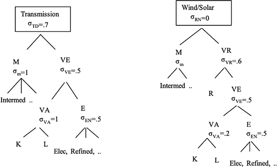
Figure A2. Structure of electricity sector. (a) Overall structure of electricity sector. (b) Structure of transmission and renewables.
Download figure:
Standard image High-resolution image
Table A4. Global warming potential.
| Global warming potential | ||||
|---|---|---|---|---|
| Species | Chemical formula | Lifetime (years) | 100 years | 20 years |
| Carbon dioxide | CO2 | — | 1 | 1 |
| Methane | CH4 | 12 ± 3 | 21 | 56 |
| Nitrous oxide | N2O | 120 | 310 | 280 |
| HFC-23 | CHF3 | 264 | 11 700 | 9100 |
| HFC-32 | CH2F2 | 5.6 | 650 | 2100 |
| HFC-125 | C2HF5 | 32.6 | 2800 | 4600 |
| HFC-134a | CH2FCF3 | 14.6 | 1300 | 3400 |
| HFC-143a | C2H3F3 | 48.3 | 3800 | 5000 |
| HFC-152a | C2H4F2 | 1.5 | 140 | 460 |
| HFC-227ea | C3HF7 | 36.5 | 2900 | 4300 |
| HFC-236fa | C3H2F6 | 209 | 6300 | 5100 |
| Perfluoro methane | CF4 | 50 000 | 6500 | 4400 |
| PFC-116 | C2F6 | 10 000 | 9200 | 6200 |
| Sulphur hexafluoride | SF6 | 3200 | 23 900 | 16 300 |
Table A5. GHGs inventory
| Gross output (bil yuan) | Non-CO2 GHGs (MtCO2e) | Real tax rate of 100¥/tCO2e non-GHGs tax | ||
|---|---|---|---|---|
| 1 | Agriculture | 10 146.46 | 10.69 | 1.0532% |
| 2 | Coal mining | 2197.50 | 4.89 | 2.2249% |
| 3 | Oil mining | 954.75 | dao0.18 | 0.1915% |
| 4 | Natural gas mining | 224.49 | 0.04 | 0.1915% |
| 5 | Non-energy mining | 1959.82 | 0.00 | 0.0008% |
| 6 | Food mfg. | 10 742.38 | 0.01 | 0.0010% |
| 7 | Textiles | 4341.45 | 0.00 | 0.0007% |
| 8 | Apparel, leather | 3618.18 | 0.00 | 0.0007% |
| 9 | Sawmills and furniture | 2361.89 | 0.00 | 0.0008% |
| 10 | Paper, printing, recording media | 3803.03 | 0.01 | 0.0030% |
| 11 | Petroleum processing | 4321.17 | 0.05 | 0.0124% |
| 12 | Chemicals | 14 451.66 | 2.43 | 0.1683% |
| 13 | Nonmetal mineral products | 6053.23 | 0.06 | 0.0099% |
| 14 | Primary metals | 12 034.62 | 0.25 | 0.0211% |
| 15 | Metal products | 4115.21 | 0.00 | 0.0002% |
| 16 | Machinery | 8477.33 | 0.00 | 0.0002% |
| 17 | Transportation equipment | 8263.63 | 0.00 | 0.0002% |
| 18 | Electrical machinery | 6302.67 | 0.17 | 0.0274% |
| 19 | Comm. equip, computer, electronic | 8052.30 | 0.01 | 0.0018% |
| 20 | Water utilities | 362.03 | 1.93 | 5.3294% |
| 21 | Other manufacturing, recycling | 813.85 | 0.01 | 0.0178% |
| 22 | Electricity, steam | 3762.75 | 0.00 | 0.0000% |
| 23 | Gas utilities | 472.77 | 0.00 | 0.0000% |
| 24 | Construction | 16 706.94 | 0.00 | 0.0001% |
| 25 | Transportation svc | 7430.19 | 0.54 | 0.0731% |
| 26 | Telecommunications, software and IT | 3321.50 | 0.00 | 0.0000% |
| 27 | Wholesale and retail | 8926.63 | 0.01 | 0.0008% |
| 28 | Hotels and restaurants | 2715.23 | 0.00 | 0.0008% |
| 29 | Finance | 7740.87 | 0.00 | 0.0000% |
| 30 | Real estate | 5070.92 | 0.00 | 0.0000% |
| 31 | Business services | 8994.47 | 0.77 | 0.0852% |
| 32 | Other services | 8610.99 | 0.00 | 0.0000% |
| 33 | Public administration | 3935.02 | 0.00 | 0.0000% |
: Carbon sequestration
We represent future sequestration technology in the following equation. Let  denote the quantity of carbon stored using a negative carbon technology, the supply function depends on the price,
  , and an index of technology that may change over time (
 ):
):
Since there are only speculative guesses about such future technologies, we assume this simple form which means that no labor or other intermediate inputs are required. A public enterprise owns this technology and receives the sales revenue,  .
.
The demand for these negative carbon services is assumed to be set exogenously by the government:
The cost of this is financed by the government, that is, regarded as another item of government final demand. However, since the government owns this enterprise, the sales receipts are added to government revenues, giving a simple accounting.
Table A6. Non-CO2 emission intensity.
| 2015 | 2030 | 2050 | 2060 | |
|---|---|---|---|---|
| Agriculture | 976.29 | 1036.03 | 1018.54 | 1018.54 |
| Coal mining | 423.81 | 336.75 | 106.60 | 5.54 |
| Oil mining | 16.83 | 15.07 | 8.80 | 5.32 |
| Natural gas mining | 4.10 | 6.41 | 6.47 | 6.26 |
| Non-energy mining | 0.14 | 0.22 | 0.22 | 0.21 |
| Food mfg. | 1.11 | 1.74 | 1.76 | 1.70 |
| Textiles | 0.25 | 0.39 | 0.39 | 0.38 |
| Apparel, leather | 0.21 | 0.32 | 0.32 | 0.31 |
| Sawmills and furniture | 0.17 | 0.26 | 0.26 | 0.25 |
| Paper, printing, recording media | 1.05 | 1.64 | 1.66 | 1.60 |
| Petroleum processing | 4.83 | 7.57 | 7.64 | 7.39 |
| Chemicals | 220.54 | 345.10 | 348.61 | 337.01 |
| Nonmetal mineral products | 5.25 | 8.22 | 8.30 | 8.02 |
| Primary metals | 23.03 | 36.04 | 36.41 | 35.20 |
| Metal products | 0.09 | 0.14 | 0.14 | 0.14 |
| Machinery | 0.18 | 0.28 | 0.28 | 0.27 |
| Transportation equipment | 0.17 | 0.27 | 0.27 | 0.26 |
| Electrical machinery | 15.90 | 24.88 | 25.13 | 24.30 |
| Comm. equip, computer, electronic | 1.39 | 2.17 | 2.19 | 2.12 |
| Water utilities | 185.26 | 348.94 | 404.22 | 413.89 |
| Other manufacturing, recycling | 1.29 | 2.02 | 2.04 | 1.97 |
| Electricity, steam | 23.98 | 37.53 | 37.91 | 36.65 |
| Gas utilities | 0.00 | 0.00 | 0.00 | 0.00 |
| Construction | 0.18 | 0.29 | 0.29 | 0.28 |
| Transportation svc | 49.11 | 76.84 | 77.63 | 75.04 |
| Telecommunications, software and IT | 0.00 | 0.00 | 0.00 | 0.00 |
| Wholesale and retail | 0.67 | 1.05 | 1.07 | 1.03 |
| Hotels and restaurants | 0.23 | 0.36 | 0.36 | 0.35 |
| Finance | 0.00 | 0.00 | 0.00 | 0.00 |
| Real estate | 0.00 | 0.00 | 0.00 | 0.00 |
| Business services | 73.91 | 115.65 | 116.82 | 112.94 |
| Other services | 0.00 | 0.00 | 0.00 | 0.00 |
| Public administration | 0.00 | 0.00 | 0.00 | 0.00 |
Notes: the unit is tCO2e/10000¥
Table A7. Relative changes in critical economic and environmental variables.
| Panel A: 2030 | Multi-GHG mitigation vs. CO2-only mitigation scenario | |||||
|---|---|---|---|---|---|---|
| Pathway | 30&60 | Zhang | BCG | Duan | Non-CO2 Tech | 20-year GWP |
| GDP | 0.01% | 0.02% | 0.04% | 0.03% | 0.00% | 0.01% |
| Consumption | 0.00% | 0.02% | 0.03% | 0.02% | 0.00% | 0.01% |
| Investment | 0.01% | 0.05% | 0.10% | 0.09% | 0.01% | 0.03% |
| Government | 0.00% | 0.00% | 0.00% | 0.00% | 0.00% | 0.00% |
| Export | 0.00% | 0.00% | −0.02% | −0.03% | 0.00% | 0.01% |
| Import | 0.00% | 0.00% | −0.02% | −0.03% | 0.00% | 0.00% |
| Tax Rate ($/tCO2e) | −0.72% | −0.76% | −1.00% | −1.01% | −0.56% | −2.10% |
| Electricity generation | 0.00% | 0.00% | 0.00% | 0.00% | 0.00% | 0.00% |
| Coal consumption | 0.01% | 0.04% | 0.16% | 0.15% | 0.01% | 0.04% |
| Oil consumption | 0.01% | 0.02% | 0.07% | 0.06% | 0.01% | 0.02% |
| Gas consumption | 0.04% | 0.12% | 0.30% | 0.29% | 0.03% | 0.12% |
| CO2 (million tCO2e) | 0.01% | 0.04% | 0.13% | 0.13% | 0.01% | 0.04% |
| CH4 emission | −0.05% | −0.16% | −0.45% | −0.43% | −0.05% | −0.09% |
| F-gas emission | −0.01% | −0.03% | −0.09% | −0.09% | −0.01% | 0.00% |
| N2O emission | −0.05% | −0.16% | −0.44% | −0.42% | −0.04% | −0.10% |
| Total non-CO2 GHG | −0.04% | −0.14% | −0.39% | −0.38% | −0.04% | −0.09% |
| Total GHG emission | 0.00% | 0.00% | 0.00% | 0.00% | 0.00% | 0.00% |
| Panel B: 2060 | Multi-GHG mitigation vs. CO2-only mitigation scenario | |||||
| Pathway | 30&60 | Zhang | BCG | Duan | Non-CO2 Tech | 20-year GWP |
| GDP | 0.41% | 0.42% | 0.56% | 0.43% | 0.27% | 1.26% |
| Consumption | 0.49% | 0.51% | 0.73% | 0.52% | 0.38% | 1.41% |
| Investment | 0.74% | 0.72% | 0.92% | 0.73% | 0.61% | 2.39% |
| Government | 0.00% | 0.00% | 0.00% | 0.00% | 0.00% | 0.00% |
| Export | −2.71% | −2.95% | −1.84% | −2.80% | −1.38% | 1.71% |
| Import | −3.15% | −3.39% | −2.19% | −3.21% | −1.63% | 1.47% |
| Tax rate ($/tCO2e) | −15.44% | −14.15% | −11.42% | −12.88% | −6.91% | −23.06% |
| Electricity generation | 0.00% | 0.00% | 0.00% | 0.00% | 0.00% | 0.00% |
| Coal consumption | 8.58% | 7.60% | 6.28% | 6.78% | 3.76% | 15.42% |
| Oil consumption | 0.70% | 0.76% | 0.78% | 0.82% | 0.36% | 3.79% |
| Gas consumption | 13.37% | 12.00% | 9.51% | 10.74% | 5.54% | 22.33% |
| CO2 (million tCO2e) | 426.39 | 408.50 | 389.06 | 394.93 | 200.50 | 332.39 |
| CH4 emission | −4.30% | −4.06% | −4.07% | −3.94% | −3.84% | −7.08% |
| F-gas emission | −1.72% | −1.99% | −1.03% | −1.91% | −0.20% | 3.74% |
| N2O emission | −3.54% | −3.33% | −3.41% | −3.24% | −2.38% | −5.94% |
| Total non-CO2 GHG | −3.56% | −3.43% | −3.27% | −3.32% | −2.80% | −5.60% |
| Total GHG emission | 0.00% | 0.00% | 0.00% | 0.00% | 0.00% | 0.00% |
Footnotes
- 4
Non-CO2 GHGs consist of methane (CH4), nitrous oxide (N2O) and fluorinated gases (F-gas). F-gas include hydrofluorocarbons (HFCs), perfluorocarbons (PFCs), sulfur hexafluoride (SF6), and nitrogen trifluoride (NF3).
- 5
A constant return of scale means firm's output increases at the same rate as firm's input, such as capital and labor. The model and data of the Global Trade Analysis Project (GTAP) is given in Corong et al [35] and at www.gtap.agecon.purdue.edu.
- 6
GWP is the cumulative radiative forcing of a unit mass of gas over a given time horizon, expressed relative to CO2. GWP provides a measure to compare warming impacts across GHGs. CH4 lasts about a decade but absorbs much more energy than CO2. The time period commonly used for GWPs is 100 years. Appendix table A4. Shows the GWPs used in our study.
- 7
The 2012 input-output table is given in NBS (2016). The benchmark IO table for 2012 is derived from detailed enterprise data, we extrapolated to the 2014 IO table using simpler aggregated data as described in Cao et al [36].
- 8
We have chosen to use U.S. patterns in our projections of these exogenous parameters because they seem to be a reasonable anchor. While it is unlikely that China's economy in 40 years time will mirror the U.S. economy of 1997, it is also unlikely to closely resemble any other economy. Other projections, such as those by the World Bank (1994), use the input-output tables of developed countries including the U.S.
- 9
In the Phoenix model (Sue Wing et al 2011), the elasticity of substitution between 'peak load' (which includes wind and solar) and 'base load' sources is also 1.
- 10
Our specification of base load and renewables follows EPPA-4, which assumes perfect substitution among the base load sources. We have, however, chosen to use an elasticity of four as used in the Phoenix model; in a similar setup, Vennemo et al (2014) use an elasticity of 20.
Supplementary data (0.1 MB XLSX)