

Abstract
The Qinghai-Tibetan Plateau (TP) accumulated a large amount of organic carbon, while its size and response to environmental factors for the whole area remain uncertain. Here, we synthesized a dataset to date with the largest data volume and broadest geographic coverage over the TP, composing of 7196 observations from multiple field campaigns since the 1980s, and provided a comprehensive assessment of the size and spatial distribution of carbon pools for both plant and soils on the TP using machine learning algorithms. The estimated soil organic carbon (SOC) storage to 1 m depth was  Pg (
Pg ( kg m−2 on average), accounting for approximately
  % of China's SOC stock on its <30% land area. There was
  Pg C stored in grassland soils (1 m), which played as the largest C pool on the TP, followed by shrubland (
 Pg) and forest (
 Pg). The estimated plant C pool was
  Pg (
Pg ( Pg in aboveground biomass (AGB) and
  Pg in belowground biomass). Soil and biomass C density presented a similar spatial pattern, which generally decreased from the east and southeast parts to the central and western parts. We found both vegetation and soil C (1 m depth) were primarily regulated by climatic variables and C input across the entire TP. However, main driving factors of the C stocks varied among vegetation types and depth intervals. Though AGB played as an important role in SOC variation for both topsoil (0–30 cm) and subsoil (30–100 cm), the strength of the correlation weakened with depth and was gradually attenuated from grassland to shrubland, and forest. The outcomes of this study provided an updated geospatial estimate of SOC stocks for the entire TP and their relationships with environmental factors, which are essential to carbon model benchmarking and better understanding the feedbacks of C stocks to global change.
Export citation and abstract BibTeX RIS

Original content from this work may be used under the terms of the Creative Commons Attribution 4.0 license. Any further distribution of this work must maintain attribution to the author(s) and the title of the work, journal citation and DOI.
1. Introduction
The Qinghai-Tibetan Plateau (TP) is the largest and highest plateau on the earth with unique vegetation types and climate conditions. The soil on the TP is a large carbon (C) reservoir because of the low soil carbon turnover rate due to cold weather [1, 2]. While the rapid warming rate in recent decades has long made it been recognized as an amplifier of global climate [3, 4], and would potentially accelerate the carbon loss to the atmosphere [5, 6]. Vegetation on the TP also plays an essential role in the regional C cycling given its high sensitivity of productivity to climate change [7, 8]. It is thus crucial for quantifying the carbon pools on the TP, clarifying their spatial patterns, as well as the dominant factors controlling the spatial variations of the C stocks [9, 10].
Great attention has been paid to the soil organic carbon (SOC) stock on the TP and its spatial pattern owning to its high carbon density. Early studies have been conducted on SOC stocks in 0–1 m depth on the TP [11–14], the size ranged from 18.37 to 49 Pg (1 Pg = 1015 g) with considerable uncertainty. These estimations were mostly based on data from China's 2nd national soil survey (mid-1980s) with sparse sampling sites. The upscaling methods (soil group area-weighted) are usually inadequate to account for spatial heterogeneity, which resulted in large uncertainties. Recent field survey campaigns have supplemented a large number of soil samplings that refer to broader geographic coverage and deeper soil cores [15–17]. Machine learning algorithms with geospatial and remote sensing information have been applied for SOC mapping to better capture the spatial heterogeneity of frozen-affected areas on the TP [2, 15, 17]. However, these studies mainly focus on grasslands [1, 18] or permafrost areas [2, 14–16]. The C stocks in forests and shrublands on the TP remain unclear. In addition, compared with soil, less attention has been paid to the vegetation C stocks on the TP regarding its small size compared with the soil C pool and the scanty of field observations [8]. Therefore, to clarify the size and spatial pattern of soil and vegetation C pools and reduce the uncertainty, it is necessary to provide an updated assessment with advanced compiled datasets and improved upscaling/mapping methodology for the entire TP.
Spatial variations in soil C are affected by environmental factors, including climate [19], land types [20, 21], soil properties [22, 23], and geomorphology [10]. While sparse sampling points or incongruous study areas usually lead to inconsistent results. For example, Yang et al [1] found a positive relation between SOC and mean annual temperature (MAT) in alpine grassland, while Mishra et al [10] claimed that the relationship was not significant in the permafrost area (mainly grassland) on the TP. In addition, previous studies primarily focused on a single vegetation type (i.e. grasslands) or specific geological region (i.e. permafrost), while lacking the exploration of the relationships between SOC and environmental factors of the entire Qinghai-TP.
To provide a comprehensive estimate of carbon stocks especially SOC across the entire TP, we collected 7196 observations from multiple field sampling campaigns and peer-reviewed articles, including 4809 measures for SOC with four depth intervals down to 2 m and 2387 sites for plant above- and belowground biomass (AGB and BGB). By integrating 48 environmental variables referred to meteorological dataset, edaphic and topographic factors and their interactions, we interpolated these site-level C densities to the regional scale using machine learning algorithms. We aimed to (a) comprehensively quantify the size and spatial distribution of C stocks on the TP and (b) clarify the main driving factors of the spatial variation in vegetation and soil carbon pools with depth.
2. Materials and methods
2.1. Study area
The Qinghai-TP lies between 26°0ʹ–39°47ʹN, 73°19ʹ–104°47ʹE, with an area of ∼2.5 × 10⁶km2 [24]. Its climate is characterized by intense solar radiation, long durations of sunshine, low temperature, and extensive diurnal temperature range. Grassland as the dominant ecosystem on the plateau occupying over 60% of the total area [25]. Forests and shrublands summed together to ∼5.35% of the land surface and scattered in the central and western TP. Barren lands were mainly distributed in the northern TP with dry and cold conditions.
2.2. Data collection
2.2.1. SOC and biomass data
We collected 4809 SOC observations and 2387 biomass data from multiple regional field sampling campaigns across the plateau since the 1980s [1, 2, 15–17], and established the most representative soil dataset to date, which covers the main vegetation types and spatial scope (see supplementary text in details). The sites distribution map is shown in figure 1.
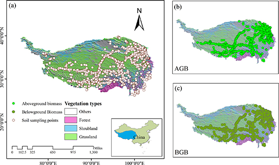
Figure 1. Distribution of sampling sites and vegetation map on the Qinghai-TP, (a) soil sampling points for SOC with depth intervals of 0–30 cm, 30–100 cm and 100–200 cm; (b) AGB sampling sites distribution; (c) BGB sampling site distribution. Vegetation types derived from China's 1: 1000 000 scale vegetation map.
Download figure:
Standard image High-resolution imageSOC stock (SOCs, kg C m−2) was calculated by the following equation (1):
where j is the soil horizon (i.e. 1, 2, 3, ..., n), SOC is SOC concentration on a mass basis (g kg−1), Cj is the volume percentage of gravel fraction, BD is the soil bulk density corrected (g cm−3), and Dj is the thickness of the jth horizon (cm). There were ∼7.5% (360/4809) SOC measurements missed their corresponding bulk density data at specific sites and layers, we hereby built an empirical (nonlinear) relationship between SOC and BD [18] to estimate the missing BD (supplementary figure S1).
Generally, each site in our dataset has multiple layers with different depth intervals. Sites with the maximum depth larger than 30 cm were used to calculate SOC stock of 0–30 cm. While sites with the maximum depth larger than 70 cm were used to estimate SOC stock of 30–100 cm, 0–100 cm, sites with depth larger than 100 cm were used to estimate SOC stock of 100–200 cm. In sum, we got 2019 sites for 0–30 cm, 1181 sites for 30–100 cm, 1302 sites for 0–100 cm, and 307 sites for 100–200 cm. These measurements are sufficient for us to assess the C stocks of the TP and further explore its controlling factors.
2.2.2. Environmental variables
To detect the relationship between environmental variables and SOC stock of TP and subsequently use a machine learning approach to predict its size and spatial pattern, we compiled an environmental data collection with 61 covariates (supplementary table S1) that refers to meteorological variables (i.e. evapotranspiration, temperature, etc), topographic indexes (i.e. slope, curvature, etc), soil physico-chemical properties (i.e. pH, clay, silt, etc) and their interactions for corresponding observation sites. For detailed information, see supplementary text. The minimum distance of paired observations was ∼3.6 km on average, considering the representative and sample density compared to former studies [2, 15], all the predictors were uniformly resampled into 5 km × 5 km resolution, and the corresponding covariates of the sampling sites were extracted for further analysis.
2.3. Principal component analysis (PCA) and reclassify the covariates
Rotated PCA (details see supplementary text) was used to reduce dimension of the independent variables and further improve the interpretation of larger groups of controls [26]. According to the variable loadings of rotated PCA and correlations among the meteorological variables (supplementary figure S2, tables S2–S5), we found temperature related 11 bioclimatic factors and precipitation related eight bioclimatic factors were always classified into different components. In addition, MAT has high correlation with variables, such as solar irradiation (RD), vapor pressure deficit (VPD) and ratio of MAT to solar irradiation (MAT_RD), and mean annual precipitation (MAP) has high correlation with variables like aridity (AI), evapotranspiration (ET), soil moisture (SM) and ratio of ET to solar irradiation (ET_RD) (supplementary tables S2–S5), we thereby grouped these principal components (PCs) related to these climatic variables into two larger categories: temperature related factors, including 11 temperature derived bioclimatic factors, RD, VPD and MAT_RD, and water related factors, including eight precipitation derived bioclimatic variables and AI, ET, SM and ET_RD. The rest PCs were further grouped into three different environmental categories including AGB, which always related with diurnal temperature range, soil physico-chemical properties and topographic factors (supplementary tables S2–S5). Machine learning algorithms was then used to build the relationships between these PCs and different C stocks and further identify the importance of each PC.
2.4. Carbon mapping
Combined with the spatial environmental covariates, we trained and tuned (supplementary text 1.3.1) the models with several machine learning algorithms, including support vector machine (SVM), random forest (RF), extreme gradient boosting and feedforward neural network. To test the model performance, we used the five-fold cross-validation approach and calculated the mean square errors as the criteria [27]. RF finally outperformed other algorithms (supplementary figure S3, table S7) and was adopted to mapping C stocks (at a resolution of 5 km) on the TP.
2.5. Uncertainty quantification of the mapping
We used two methods to quantify the uncertainty of our estimate, absolute uncertainty and relative uncertainty (details see supplementary text). Briefly, for the former one, we used a quantile regression forest approach to calculated the interquartile of each pixel (difference between the 75th and 25th percentiles), further the summed and averaged value of the 25th and 75th percentiles were used to represent the uncertainty of OC stocks on the TP [2]. To get the relative uncertainty, the sensitivity and model structure uncertainty were then summed up to represent the total uncertainty, which then was divided by the median values of each pixel to obtain the relative uncertainty [2, 28, 29].
2.6. Statistical analysis
If the P-value of Kolmogorov Smirnov [30] test was smaller than 0.05, we used log transformation for the data for further model establishing and analysis. Biomass C, including AGB and BGB, in this study were all transformed into base-10 log scale for further analysis. They were transformed back after model prediction. All statistical analysis were conducted in R platform [31]. The packages we mainly used were listed in supplementary text.
3. Results
3.1. Relationships between different carbon stocks and climate
The relationship between C stocks (bin-averaged) and climatic factors varied with vegetation types (figure 2). Specifically, both grassland AGB and BGB showed a significant positive tendency with MAP (p < 0.01, figure 2(a)), but their correlations with MAT were sharply weakened (figure 2(d)). While for shrubland, a decreasing relationship with MAT was found for both its AGB and BGB (p < 0.01, figure 2(e)). In addition, only AGB in forest showed a positive relationship with MAP (p < 0.01, figures 2(c) and (f)).
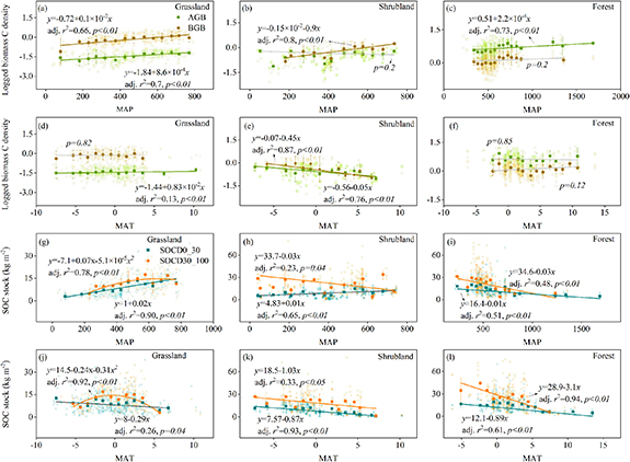
Figure 2. Relationships between different ecosystem carbon stocks and climate variables. The AGB and BGB carbon content of grassland, shrubland and forest to MAP (a)–(c) and MAT (d)–(f). SOC density (SOCD) of topsoil (0–30 cm) and subsoil (30–100 cm) to MAP (g)–(i) and MAT (j)–(l). A base-10 log scale is used for the Y-axis of panel (a)–(f). Circles and squares in (a)–(f) represent AGB and BGB, respectively. Circles and squares in (g)–(l) represent SOCDs of topsoil (0–30 cm) and subsoil (30–100 cm), respectively. Points that used to fit the linear and second order regression model were the averaged values of C density within bin intervals of MAT/MAP. Specifically, the bin interval was 50 mm for MAP and was 1 °C for MAT.
Download figure:
Standard image High-resolution imageMoreover, the correlations between SOC and MAP gradually shifted from positive in grassland (p < 0.01) to negative in forest (p < 0.01) for both topsoil and subsoil (figures 2(g) and (i)). SOC stock in shrubland showed an opposite trend to MAP at the two depth intervals, increasing in topsoil and decreasing in subsoil. However, the response of SOC stock to MAT was almost synchronized at both soil layers (figures 2(i)–(l)), which all showed a negative relationship with MAT for the three vegetation types.
3.2. The relative importance of environmental variables to vegetation and soil C stocks
The primary governing environmental category differs for vegetation and soil C stocks on the TP. For AGB, temperature and water related factors contributed the most to its spatial distribution, taking half of its variation across the TP (figure 3(a)), indicating the dominant role of climatic variables in shaping amount of AGB. While for the individual land covers, the main driving environmental category changed from precipitations related factors in grassland to soil properties and temperature related factors in shrubland and forest (figure 3(a)), respectively.
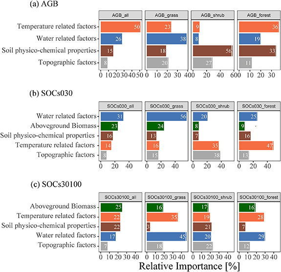
Figure 3. Relative accumulative contributions of environmental categories to different carbon stocks on the TP. (a) Relative importance of environmental categories to AGB for all sites, grassland, shrubland, and forest, respectively. (b) Relative importance of environmental categories to topsoils (0–30 cm) for all sites, grassland, shrubland, and forest, respectively. (c) Relative importance of environmental categories to subsoils (30–100 cm) for all sites, grassland, shrubland, and forest, respectively. Relative importance of each environmental category was obtained by summing up the importance of each corresponding PC (supplementary figure S4). Relative importance of AGB was token out separately, which was derived by multiplying the importance of its corresponding PC by its loading to the PC (supplementary tables S2–S5). Error bar represent standard deviation of the relative contribution from five replicates of model run.
Download figure:
Standard image High-resolution imageFor SOC stock, AGB played a primary role for both topsoil (0–30 cm) and subsoil (30–100 cm) (figures 3(b) and (c)), demonstrating the importance of plant-derived C input to SOC stocks on the TP. For topsoil, both AGB and water related factors (MAP, etc) showed positive effect on the SOC stocks across the TP, while temperature related factors like temperature fluctuation ratio of monthly to yearly (isothermality, supplementary figure S5(e)) almost showed a linear negative effect on SOC stocks. However, the dominant driving environmental category varied among different vegetation types (figure 3(b); supplementary figures S4(e)–(h)), which changed from water related factors in grassland to topographic factors, temperature related factors in shrubland and forest (figure 3(b)), suggesting divergent controlling factors among land covers on the TP.
Unlike topsoil, besides AGB, there were no exceptional environmental categories contributing to subsoil SOC stocks. Categories such as temperature related and soil physico-chemical properties had almost the same contribution to SOC in sublayers throughout the TP (figure 3(c)). Moreover, the dominant regulatory categories were relatively consistent for the individual land cover (figure 3(c)), which were all referring to water and temperature related factors, revealing a relative complex mechanism in regulating the SOC in deeper soils. Specifically, the influence of individual PCs on different SOC stocks with depth exhibited the same trend, which all increased with precipitation and decreased with temperature related factors (supplementary figures S4(i)–(l)).
3.3. Size and spatial patterns of vegetation and soil C stocks on the TP
The spatial distribution of both vegetation and soil C densities presented a similar pattern. Namely, the C density decreased from the east and southeast parts to the central and western parts and then increased again at the northwest edge within Xinjiang Uygur autonomous region (figures 4(a)–(c) and (g)–(i)). While, their uncertainties showed an opposite tendency between plant and soil carbon pools (insets of figures 4(a)–(c) and (g)–(i)). The uncertainties of vegetation C density exhibited a similar pattern with its density distribution, suggesting proportional uncertainties to their C density. While the highest uncertainty for soil C densities within 1 m depth was concentrated in the northwest part and then decreased to the eastern part (insets of figures 4(g) and (h)).
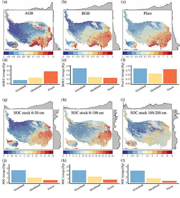
Figure 4. Spatial pattern of different C stocks (kg m−2) on the TP and their C storage size within the three vegetation types. Spatial pattern of (a) AGB C stock, (b) BGB C stock, (c) plant C stock, (g) 0–30 cm SOC, (h) 0–100 cm SOC, (i) 100–200 cm SOC. Total C stocks (Pg) of grassland, shrubland and forest in (d) AGB, (e) BGB, (f) plant, (j) 0–30 cm soil, (k) 0–100 cm soil, (l) 100–200 cm soil.
Download figure:
Standard image High-resolution imageThere was a total of  Pg C (confidence interval of upper and lower estimate indicated 75th and 25th percentiles to quantify the prediction uncertainty) stored in vegetation on the TP. Of which
  Pg was allocated to AGB and
  Pg was assigned to BGB (figures 4(a)–(c)). The average carbon density of AGB was increased from 0.10 kg m−2 in grassland to 0.52 and 2.86 kg m−2 in shrubland and forest, respectively. Correspondingly, their carbon stock size increased from
  Pg in grassland to
  and
and  Pg in shrubland and forest. In contrast, the carbon stored in BGB was decreased from
  Pg in grassland to
  and
and  Pg in forest (figures 4(d)–(f)).
The estimated SOC stock on the entire TP was  Pg (
Pg ( kg m−2 on average) for 0–100 cm soil and
  Pg for 0–200 cm depth (
 kg m−2 on average). Though the average SOC stock (0–100 cm) increased from grassland (9.95 kg m−2) to forest (19.12 kg m−2), the opposite trend of their total storage was found, the largest SOC pool was grassland soils (
 Pg, 48.5%), of which
  Pg stored in alpine meadow and
  Pg stored in alpine steppe, followed by shrubland (
 Pg, 23.5%) and forest (
 Pg, 11.6%) (figures 4(f)–(h)). There was
  Pg SOC stored in 0–30 cm depth, which accounted for 44.57% of 0–100 cm SOC storage, and of which
  Pg stored in grassland (
 Pg stored in alpine meadow and
  Pg stored in alpine steppe),
  Pg in shrubland and
  Pg in forest, respectively. All indicated that grassland, especially its alpine meadow system, played as the largest C reservoir to the TP.
3.4. Relationships between vegetation and soil C stocks
SOC and AGB were closely related on the TP, especially for grassland and shrubland (figure 5). SOC increased significantly with the increase of AGB in grassland for the topsoil (p < 0.01) (figure 5(a)). Though the strength of the correlation (bin averaged) decreased in deeper soil (30–100 cm), the coefficient still at a high level (0.78) (figure 5(b)). There was also a strong positive correlation between AGB and SOC in shrubland in topsoil (0–30 cm), of which the coefficient was 0.70 (p < 0.01). For the forest, though there was a negative trend between AGB and SOC, they are not statistically significant (p > 0.05) (figure 5).
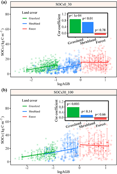
Figure 5. Relationship between AGB carbon stock and SOC stocks in 0–30 cm (a) and 30–100 cm (b). The inserts represent the correlation coefficient of AGB to SOCs with depth for the three vegetation types. A base-10 log scale is used for the X-axis of (a) and (b).
Download figure:
Standard image High-resolution image4. Discussion
4.1. Carbon stocks on the TP
Based on the unique compiled dataset, widely collected environmental variables, and the advances of machine learning (RF) approach, this study provided a comprehensive assessment of the TP for both its biomass and soil carbon pools. The total estimated biomass carbon stock was  Pg, which accounted for 23.4% of China's total vegetation carbon stock (figure 6(a)). The estimated biomass C stock size of grassland was 0.86 Pg, which accounted for 63.7% of China's total grassland biomass C size (1.35 Pg from Tang et al [34]), this proportion was similar with the findings by Fan et al (56.4%) [35], but the amount was much lower than theirs (1.87 Pg). Our results of biomass C densities were higher in shrubland and lower in forest compared with China's average value by Tang et al [34] (1.07 vs 0.64 kg m−2 in shrubland, and 4.2 vs 5.32 kg m−2 in forest).
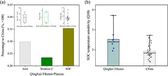
Figure 6. Comparison the C stock size and SOC temperature sensitivity on the Qinghai-TP to China. (a) Percentage of biomass C and SOC stock (1 m depth) on the TP to that amount of China. The box insets in the upper middle represented values of area, biomass C and SOC storage (medians) in China, which were collected from previous studies. Of which the medium value was used to represent the benchmark value of China. (b) Comparison of SOC temperature sensitivity on the TP to China. Data used were derived from published articles. Detailed information was provided in supplementary materials.
Download figure:
Standard image High-resolution image
The estimated SOC stock of the entire TP was  Pg C (1 m depth), with an average density of
  kg C m−2, correspondingly accounting for
  % (25%–75% quantile) of China's SOC stocks (median = 86.09 Pg) (figure 6(a)), and ∼2.2% of global SOC stock (synthesized ∼1448.9 Pg) [36, 37]. This size was much similar to Jiang's et al [14] report (32.79 Pg with 12.68 kg m−2 on average) but lower than the estimates of Fang [13] (38.4 Pg for 0–0.72 m depth) and Tian et al [12] (49 Pg for 0–0.75 m depth) (table 1). To compare with the results from earth system models (ESMs), we chose ten ESMs derived from Coupled Model Intercomparison Project v.5 over the TP, and found our estimates (0–100 cm) was similar with the averaged prediction (∼29.32 Pg C) of the ten ESMs (supplementary figure S6). However, almost all of these ten ESMs failed to capture the spatial pattern of SOCs distribution [38], our outputs could be provided as a benchmark for future carbon model prediction on the TP.
Table 1. Comparison the estimates of SOC stocks on the TP.
| Depth (m) | Study area | N | Area (106 km2) | Methods | SOCD (kg m2) | SOCS (Pg) | Reference |
|---|---|---|---|---|---|---|---|
| 0–0.3 | Grassland | 135 | 112.82 | Linear regression with satellite observations | 4.42 | 4.99 | [1] |
| Grassland | 135 | 112.82 | Linear relationship with satellite observations | 3.9 | 4.4 | [32] | |
| Permafrost (mainly grassland) | 103 | 114.4 | Mean value with area | 4.63 | — | [9] | |
| Permafrost (mainly grassland) | 200 | 148 | Mean value with area | — | 6.05 (5.74–6.39) | [16] | |
| Permafrost (mainly grassland) | 173 | 110 | Regression-kriging interpolation | 6 (3.5–9) | 7 (4–10) | [10] | |
| Grassland | 2019 | ∼157 | Machine learning—RF | 5.0 | 7.8 | This study | |
| 0–1 | Grassland | 135 | 112.82 | Linear regression with satellite observations | 6.52 | 7.36 | [1] |
| Permafrost (mainly grassland) | 173 | 114.4 | Machine learning—SVM | 7.44 (6.38–8.68) | 8.51 (7.3–9.93) | [2] | |
| Permafrost (mainly grassland) | 200 | 148 | Mean value with area | — | 12.73 | [16] | |
| Permafrost | 190 | 135 | Mean value with area | — | 17.3 ± 5.3 | [33] | |
| Permafrost (mainly grassland) | 114 | 110 | Regression-kriging interpolation | 8 (6–9.5) | 9.2 (7–11) | [10] | |
| Frozen ground | 158.8 | Upscaling with soil subgroups | 11.21 | 17.79 | [14] | ||
| Grassland | 1302 | ∼157 | Machine learning—RF | 9.95 | 15.52 | This study | |
| Permafrost | 1302 | ∼117 | Machine learning—RF | 9.25 | 10.74 | This study | |
| 1–2 | Permafrost (mainly grassland) | 114 | 110 | Regression-kriging interpolation | 2 (0.3–5) | 2.5 (0.4–6) | [10] |
| Permafrost (mainly grassland) | 200 | 148 | Upscaling with land covers | — | 3.57 (1.3–6.66) | [16] | |
| Permafrost | 190 | 135 | Mean value with area | — | 10.6 ± 2.7 | [33] | |
| Permafrost | 307 | 117 | Machine learning—RF | 2.95 | 3.41 | This study | |
| 0–2 | Permafrost (mainly grassland) | 173 | 114.4 | Machine learning—SVM | 10.68 (9.1–12.51) | 12.22 (10.41–14.31) | [2] |
| Permafrost (mainly grassland) | 200 | 148 | Upscaling with land covers | — | 17.07 (11.34–25.33) | [16] | |
| Permafrost (affected region) | — | — | Review | — | 19 ± 6.6 | [6] | |
| Permafrost (affected region) | 190 | 135 | Mean value with area | 27.9 | [33] | ||
| Permafrost | 307 | ∼117 | Machine learning—RF | 6.09 | 13.88 | This study | |
| 0–3 | Permafrost | 1114 | Machine learning—SVM | 15.4 (14.4–16.4) | 36.6 (34.3–38.9) | [15] | |
| Permafrost | 314 | Machine learnings—RF | 6.14 | 15.33 | [17] | ||
| Frozen ground | 158.8 | Upscaling with soil subgroups | 25.76 | 40.89 | [14] | ||
| Actual depth | Entire TP | the 2nd National Soil Survey | 255.1 | Upscaling with soil subgroups | 7.2 | 18.37 | [12] |
| 0–0.72 | Entire TP | the 2nd National Soil Survey | 197 | Upscaling with soil subgroups | 19.5 | 38.4 | [13] |
| 0–0.75 | Entire TP | 124 | 162.7 | Mean value with area | — | 49.0 | [12] |
| 0–1 | Entire TP | 144 subgroups | 258.7 | Upscaling with soil subgroups | 12.68 | 32.79 | [14] |
| 0–3 | Entire TP | 144 subgroups | 258.7 | Upscaling with soil subgroups | 28.45 | 73.6 (63.9–83.3) | [14] |
| 0–1 | Entire TP | 7196 | 273 | Machine learning—RF | 11.72 | 32.01 | This study |
| 1–2 | Entire TP | 307 | 273 | Machine learning—RF | 2.96 | 8.1 | This study |
Though the larger proportion of SOC on the TP compare to its area (figure 6(a)), the sensitivity of which to warming such as Q10 was found to be ∼20.7% larger than the average level of China (2.32–1.93) (figure 6(b)), suggesting its vulnerability in response to climate warming on the TP. Process-based model (ORCHIDEE) has indicated that a 2 °C warming could invoking ∼10% of SOC stock lost (1.2 Pg) in grassland, which would make the TP a weak C source [39]. While Chen et al [40] synthesized 65 publications and found the total amount of SOC on the TP would not change under warming, the lost C induced by enhanced respiration could be compensated by increased plant biomass and dissolved OC. Concerning the uneven distribution of current warming experimental sites on the TP, more attention should be further focused on its central and west part and besides grassland to obtain a more comprehensive assessment of its SOC feedbacks to global warming.
SOC stored in the grassland was  Pg, which accounted for 64.5% of China's grassland carbon size (24.03 Pg), indicating the large contribution (∼64%) of TP's grassland to China's grassland C stock on ∼55% of its area [34]. The large size of SOC reservoir in grassland primarily due to the slow OC decomposition rate by low temperature in most alpine grassland regions [2, 10, 19]. To make a further comparison, SOC storage of alpine grassland was estimated (14.07 Pg, 9.92 kg m−2 on average), and the amount was almost two times the size of Yang et al [1] results for 0–1 m (7.36 Pg, 6.52 kg m−2 on average). Additionally, we overlay a digital permafrost distribution map on our predicted maps, and found that there were
  ,
,  , and
, and  Pg C stored in 0–0.3 m, 0–1 m and 1–2 m in permafrost regions, respectively, which were all fell into the range of previous estimations, but mainly at a high level for each depth interval (table 1).
Differences between our estimates to previous studies could be mainly induced by three possible reasons. Firstly, the dataset was unprecedently improved for both its data volume and geographical coverage, making the data more representative and minimizing the uncertainties [10, 15]. In particular, we have appended a large number of measurements from regional field works conducted in shrub and forest ecosystems, which were rarely concerned by former estimates. Moreover, number of observations from permafrost regions were complemented recent years, which has largely increased the average value of SOC density (SOCD) in grassland than before (increased to 6.96 and 9.95 kg C m−2 for 0–0.3 m and 0–1 m, respectively). Secondly, algorithms have a non-negligible effect on regional SOC prediction. The machine learning approach used in this study was expected to have better performance than traditional up-scaling methods [2]. A recent work by Liu et al [41] used ensemble machine learning algorithms mapping China's soil information, and achieved more accurate predictions compared with previous soil maps like the harmonized world soil database (HWSD, v1.2), which produced by linking raster to harmonized soil property data. Thirdly, differences in scale may also result in estimation deviations among vegetation types. For instance, area of alpine grassland used in this study was ∼1.42 × 10⁶ km2 which was larger than 1.13 × 10⁶ km2 that used in Yang et al [1].
Though machine learning has proven to have great advantages in OC mapping [2, 17], this study still has uncertainties. For biomass C stocks, the large uncertainty from forest AGB and grassland BGB suggested that additional observations in above ground forest and belowground grassland are needed in the future (figures 4(a)–(c)). For SOC stocks, the uncertainty decreased for 0–100 cm compared with 0–30 cm, which was consistent with the tendency from Ding et al [2] and Jiang et al [42]. While the uncertainty increased sharply when it concerned 100–200 cm depth, which was in accordance with the findings by Mishra et al [10], who claimed the uncertainty was much higher at 100–200 cm depth interval on the TP's permafrost region. These above uncertainties could mainly be resulted from the lack of sampling points, which again suggested the necessity of supplemental samplings for the non-sampling areas and deeper soils.
4.2. Driving factor for different carbon stocks in the TP
Ecological correlation does not necessarily imply causation. Temperature related factors, specifically the mean diurnal temperature range (Tdr), was shown as the primarily factor negatively controlling AGB across the TP (figure 3(a), supplementary figures S4 and S5). Usually, vegetation through physiological processes like evapotranspiration and biomass energy absorption modifying ambient air temperature during daytime, and releasing the absorbed energy to atmosphere during nighttime affecting ambient air temperature, and thus influence the Tdr. Therefore, Tdr, as an indicator, is regulated by interaction among plant and surrounding factors like solar irradiation, VPD etc [43]. On the TP, the spatial pattern of AGB was asynchronous with the Tdr, which increased from forest in southwest to barren desert steppe in west central part (figure 4(a)). From this point of view, the dominant driving factor for AGB should be water related factors on the TP (supplementary figure S4(a)). However, our result implied that Tdr can be used as an effective covariate for AGB prediction on the TP.
Our results suggested that AGB and water related variables presented as the key categories for the topsoil (0–30 cm) SOC stock, which was consistent with former studies [1, 44, 45]. SOC of topsoil on the TP was susceptible to precipitation because it could increase organic C input into the soil by enhancing plant productivity. For subsoil (30–100 cm), we found AGB and climatic variables still played as a dominant role in driving its SOC, though the accumulative contribution of soil physico-chemical properties increased (figure 3(c)). This result appears to be inconsistent with the early findings on a global scale (with ∼2700 soil profile) [19] which claimed a switched importance of SOC driving factors with depth, and emphasized the importance of edaphic factors for deep soils. However, Luo et al [46] recently used an updated global soil dataset (141 581 soil profile) detecting the controlling factors and found the importance of climatic variables did not show a decreasing trend with depth. Additionally, Mishra et al [10] used the regression kriging method (AGB was not included) also suggested the importance of climate to deep SOC which found precipitation could explain the largest portion of the SOC variation for both 0–0.3 m (47%) and 0–1 m (24%) SOC on the TP. It is important to note that the relative high SOCD the TP was mainly attributed to its cold weather. As the C output pathway was inhibited by low temperature, the mass C balance should be dominated by C input from plant which was primarily controlled by climatic variables (figure 3(a), supplementary figure S4(a)). In addition, from the data aspect, the topsoil (0–30 cm) and subsoil (30–100 cm) showed a high correlation (figure S7) and also a similar spatial pattern (figures 4(g)–(h)), therefore our findings, these two layers were synchronized on the main driving factor, should be reasonable. However, C stability in subsoils might still be controlled by edaphic related factors rather than climatic variables. A recent study used radiocarbon (Δ14C) measurements detecting controlling factors on C persistence on the TP's grassland, and found the dominant factor for SOC persistence changed to mineral properties in subsoil due to a decreased root C input [45]. While evidence from temperature control experiments have also demonstrated that deep SOC had higher sensitivity (Q10) to warming than topsoils [47, 48], and was vulnerable to climate warming [49]. Given the large uncertainty and vulnerability of SOC to climate, more field observations and manipulative experiments of whole-soil profile should be paid to clarify the feedbacks of deep soils to the ongoing climate change.
For vegetation types, the dominant driving factors of topsoil SOC in grassland were coming from water related categories (supplementary table S5), which was in accordance with former studies [1, 10]. While for shrubland, the key driving factors transformed into temperature related variables. The significant negative relationship between temperature related variables (supplementary table S5) and SOC stock in shrubland in this study was consistent with the findings from shrubland on a global scale [19, 50], which indicated an increasing risk for C loss in shrubland due to warming stimulated biological degradation. The reason might be that alpine shrubs are mainly distributed on shady slopes and foothills with lower solar radiation and thus low temperature and water consumption. Therefore, water becomes no longer a limit factor and the temperature becomes the main constraint of the shrub ecosystems.
4.3. Relationship between different C stocks
The tendency between plant productivity and SOC varies with vegetation types. The correlation coefficients decreased from grassland to shrubland and disappeared in forest (figures 5(a) and (b)). Plant productivity (i.e. AGB) in grassland was mainly controlled by water related variables (figure 3(a)), and the low temperature further constrains the microbe activities for SOM decomposition. Therefore, plant productivity was closely related to its SOC stocks in grassland, which has also been demonstrated by remote sensing observations [1, 18]. Whereas, for shrubland, temperature related variables was the main driver on its topsoil SOC which mainly affect the C loss path [50]. Therefore, the relationship between AGB, which determine C input, and SOC was weakened. For forest, only a small portion of its AGB, mainly leaves, fall on the ground and has been involved in the C cycle every year, resulting in no significant relationship between them.
Besides, the strength of the correlations between AGB and SOC weakened with depth. For subsoil (30–100 cm), only grassland exhibited a significant (p < 0.01) relationship between AGB and SOC, with a decreased R2 (figure 5(b)). Which confirmed by previous findings that the importance of C input from plant decrease with increased soil depth [19, 45]. However, AGB still played a dominant role in shaping subsoil SOC distribution, indicating that the importance of plant C input for deep SOC (to 1 m) was non-negligible on the TP. The similar contribution of other environmental categories (i.e. temperature and soil properties) suggested a relative complex regulatory environment for the deep soils [51]. In sum, our findings implicated that the responses of SOC to future climate change may differs depending on interactions between vegetation types and regional climate conditions.
Acknowledgments
This study was sponsored by the Second Tibetan Plateau Scientific Expedition and Research Program (Grant No. 2019QZKK0405), China Postdoctoral Science Foundation (Grant No. 2020M672684), Key R&D Program of Hainan (Grant No. ZDYF2022SHFZ042), and the start-up fund of Hainan University (Grant No. KYQD(ZR)21096). We gratefully acknowledge the valuable suggestions provided by the anonymous reviewers of this manuscript, and the expert guidance of the Associate Editor.
Data availability statement
The data that support the findings of this study are available upon reasonable request from the authors.
Conflict of interest
None declared.
Supplementary data (1.9 MB PDF)