
Abstract
Objective. Neuroimaging is one of the effective tools to understand the functional activities of the brain, but traditional non-invasive neuroimaging techniques are difficult to combine both high temporal and spatial resolution to satisfy clinical needs. Acoustoelectric brain imaging (ABI) can combine the millimeter spatial resolution advantage of focused ultrasound with the millisecond temporal resolution advantage of electroencephalogram signals. Approach. In this study, we first explored the transcranial modulated acoustic field distribution based on ABI, and further localized and decoded single and double dipoles signals. Main results. The results show that the simulation-guided acoustic field modulation results are significantly better than those of self-focusing, which can realize precise modulation focusing of intracranial target focusing. The single dipole transcranial localization error is less than 0.4 mm and the decoding accuracy is greater than 0.93. The double dipoles transcranial localization error is less than 0.2 mm and the decoding accuracy is greater than 0.89. Significance. This study enables precise focusing of transcranial acoustic field modulation, high-precision localization of source signals and decoding of their waveforms, which provides a technical method for ABI in localizing evoked excitatory neuron areas and epileptic focus.
Export citation and abstract BibTeX RIS

Original content from this work may be used under the terms of the Creative Commons Attribution 4.0 license. Any further distribution of this work must maintain attribution to the author(s) and the title of the work, journal citation and DOI.
1. Introduction
The brain is the most important and complex organ in the human body, and exploring its functional activities is beneficial for humans to have a clear understanding of their state and to treat neurological disorders. Safe and accurate functional brain imaging is one of the key technologies for in-depth study of brain science [1]. Currently, functional brain imaging techniques include single-unit activity, multi-unit activity, local field potentials, and electroencephalography, which are invasive neurological recording techniques that require surgically implanting electrodes into the brain to obtain signals, which have relatively high spatial and temporal resolution [2]. Non-invasive imaging techniques such as functional magnetic resonance imaging (fMRI), electroencephalogram (EEG) and magnetoencephalography (MEG) are not yet capable of directly observing the activity of target neurons. fMRI is based on the blood-oxygen level dependent effects of neural activity, which are reflected by the local magnetic field changes. These changes are caused by increased oxygen consumption and blood flow occurring in excitable brain regions. However, its low temporal resolution makes it difficult to capture neuronal activity [3], rendering it insufficient for timely brain function imaging. MEG and EEG have high temporal resolution for capturing dynamic brain activity. However, the volume conduction effect in brain tissue results in low spatial resolution, which does not allow for accurate localization of induced excitatory neuronal areas or focal areas of abnormal discharges [4].
In recent years, researches have shown that acoustoelectric brain imaging (ABI) can combine the advantages of both the millimeter-level high spatial resolution of transcranial focused ultrasound (tFUS) and the millisecond-level high temporal resolution of EEG signals [4]. ABI is expected to be a functional brain imaging technique for exploring the working mechanisms of the nervous system. It is currently receiving the attention of many researchers in the areas of neuron localization and deep brain stimulation electrode current mapping. In 2016, Qin et al first demonstrated the feasibility of ABI to localize neuronal firing in the brain [5, 6]. In 2018, Burton et al demonstrated the feasibility of mapping current source activity in the rat hippocampus using ABI based on invasive and non-invasive electrodes [7]. In 2020, Zhou et al tested multi-source ABI with different frequencies and amplitudes based on salt water experiments, and the results proved that current sources with different parameters could be clearly imaged, and also the corresponding features could be effectively extracted from the acoustoelectric (AE) signal, which verified the feasibility of multi-source ABI [8]. In 2021, Song et al conducted a steady-state visual evoked potentials (SSVEPs) experiment in living rats based on ABI, and the experimental results showed that the decoded AE signal had high amplitude responses at both fundamental and harmonic of the visual stimulus frequency, and this experimental study realized the first millimeter spatial resolution SSVEP measurement in living rats [9]. In 2022 Zhang et al used FUS irradiation to simulate the dipole of neuronal discharge, and the simulation and experimental results showed that the localization and decoding results were highly consistent with the preset parameters, and the dipole localization error was less than 0.3 mm [10].
It should be noted that ABI requires tFUS to provide spatial position information in the intracranial focal domain, so how to overcome the acoustic field aberrations caused by the cranial structure and acoustic properties is also one of the difficult problems that need to be solved by ABI technology. Many existing ABI studies use a single array self-focusing transducer and ignore the effect of the skull. They believe that the geometric focus of the single array transducer is the actual focus position. This belief is approximately feasible in saline experiments and tissue-mimicking phantom experiments. However, due to the strong acoustic attenuating and non-homogeneous characteristics of the skull, the ultrasound waves are susceptible to the risk of focus shifting and defocusing after the cranial transcranial [11]. This susceptibility ultimately leads to a large discrepancy between the ABI results and the actual situation. To this end, we have investigated key aspects of ABI such as transcranial acoustic field modulation and dipole localization and decoding based on an independently constructed 128-array ultrasonic phased array transducer experimental platform under both pure water and simulated skull conditions.
2. Theory
2.1. Acoustic field simulation and modulation methods
2.1.1. Numerical simulation methods for acoustic field
The nonlinear Westervelt equation is used to describe the acoustic field in numerical simulations [12, 13]. It incorporates the effects of nonlinearity, attenuation, reflection and scattering and can be written as:
where  is the acoustic pressure,
  is the time,
  is the thermoviscous diffusivity,
  is the nonlinear coefficient,
  is the angular frequency, and
  is the ultrasonic center frequency. The equation was calculated by the finite difference time domain (FDTD) method in 3D Cartesian coordinates with a spatial step of 0.1 mm and time step of 10 ns. The Mur first-order absorbing boundary condition was used at the boundary to avoid ultrasonic reflections [14]. Here the effect of shear waves is ignored since most of the incidence angles are less than 20° and the maximum incidence angle is less than 25° [15].
2.1.2. Transcranial acoustic field modulation method
Transcranial acoustic field modulation is realized based on the time reversal method. Specifically, a virtual point source  is first set up at the intracranial target focal point, and the acoustic pressure of the ultrasound emitted by this point source propagating to the center position of each array of the transducer is calculated by numerical simulation. The signal
  received by array
  is then inverted in
  in a time sequence to obtain the inverted signal
  . Next, the corresponding fitting parameters are set based on the least squares function fitting method to realize the extraction of the initial phase of the target fitted signal, and the initial phase of array element
  is obtained as
  . Finally, under the same acoustic pressure
  , each array of the transducer realizes transcranial phase-modulated focusing at the target focal point based on different initial phases
  , so the excitation signal of each array is:

2.2. ABI method
2.2.1. AE effect
The most basic imaging principle of ABI is the AE effect. The AE effect is a phenomenon in which the current passing through an electrolyte under the coupling of acoustic and electric fields is subjected to the periodic modulation of the focused acoustic pressure field, causing the local conductivity of the medium to vary with the ultrasonic rhythmicity [16]. The phenomenon was first discovered in 1946 by Fox et al. Ultrasound can periodically change the electrical conductivity of salt water by pressure [17]. The next study found that ultrasound affects the dielectric conductivity mainly by changing the physical and chemical properties of the medium such as molar concentration, ion ionization equilibrium and ion mobility [18–20].
2.2.2. ABI principle
The AE effect indicates that the change in medium conductivity  due to FUS is [21, 22]:
where  is the change in medium conductivity,
  is the intrinsic conductivity,
  is the change in acoustic pressure, and
  is the interaction constant, which is on the order of
  in a 0.9% NaCl solution.
The voltage  obtained from the measurement of lead numbered
  in the EEG acquisition is generally expressed as:

where  is the current density distribution of lead
  and
and  is the current density distribution of neurons.
Based on equation (3), the local conductivity of the medium at the FUS modulation is:
Substituting (5) into (4) gives
where  is the low-frequency EEG signal of
  and
and  is the high-frequency AE signal. The high-frequency AE signal acquired at the point
  on the plane of FUS irradiation after high-pass filtering is:
where  is the ultrasonic beam pattern,
  is the acoustic pressure amplitude,
  is the pulse waveform, and
  is the acoustic velocity.
Equation (7) can be simplified as [23]:

where  ,
,  . When
  , equation (8) becomes:

The minimum paradigm estimate of the current density  at point
  is:
is:
where Moore–Penrose pseudoinverse  .
.
Therefore, the divergence of the neuronal current density distribution  is:
is:

From the current density distribution of the dipole, it can be seen that the current density at the dipole is the largest, and as the current spreads outward, the current density in the region farther away from the dipole is smaller. From the AE effect, it can be seen that when FUS irradiates the target area at a certain frequency (center frequency/pulse repetition frequency), the AE signals generated in the region of higher current density are stronger, while the AE signals in the region of lower current density are relatively weaker. Therefore, the ABI can localize the dipole position based on the AE signal value at each point of the ultrasound scan, and the larger the AE signal amplitude, the closer the localization position is to the actual position of the dipole.
3. Materials and methods
3.1. Experimental platform for acoustic field modulation
3.1.1. Numerical simulation model
Figure 1 shows the schematic diagram of the numerical simulation model. The simulation model mainly consists of a 128-array ultrasound transducer, an acrylic simulated skull and water. Among them, the diameter of the transducer opening is 100 mm, the radius of curvature is 60 mm, and the diameter of the array is 4 mm; the thickness of the acrylic plate is 8 mm, the radius of curvature is 100 mm, and it is 15 mm from the surface of the transducer. The numerical simulation area is 100 mm × 100 mm × 100 mm. The numerical simulation parameters are shown in table 1.

Figure 1. Schematic diagram of the numerical simulation model.
Download figure:
Standard image High-resolution image3.1.2. Experimental setup
Acoustic field tests are conducted based on the 128-array ultrasound phased array experimental platform (passed assembly error test) shown in figure 2, in which figure 2(a) shows the overall system diagram, which mainly includes the upper control module (the red circles represent the transmitting arrays and the blue circles represent the receiving arrays), high precision oscilloscope, power amplifier module, data acquisition module, 3D adjustment frame, positioning module, and acoustic field scanning module; figure 2(b) shows a partial enlargement of the positioning module, which utilizes a laser collimator to perform the geometrical focal point and simulated cranial localization; and figure 2(c) shows a partial enlargement of the acoustic field scanning module, which mainly includes the hydrophones, bone plate fixation device, acrylic plate, and transducer. In this case, the thickness of the acrylic plate is 8 mm, the radius of curvature is 100 mm, and the distance of the acrylic plate from the transducer is 15 mm, and its center is aligned with the center of the transducer along the acoustic axis. The acquisition range is the XZ section enclosed by the four points (−4, 0, 55), (4, 0, 55), (4, 0, 65) and (−4, 0, 65), with a scanning length of 8 mm in the X direction and 10 mm in the Z direction, and a scanning step of 0.1 mm.
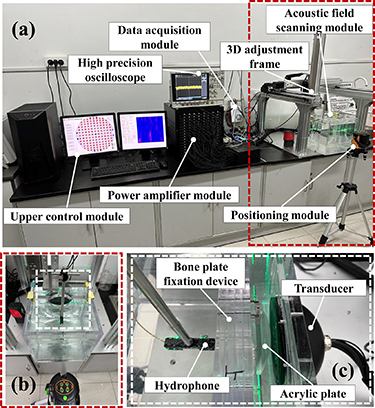
Figure 2. Ultrasonic phased array transducer experimental platform. (a) Overall system diagram. (b) Partial enlargement of the positioning module. (c) Partial enlargement of the acoustic field scanning module.
Download figure:
Standard image High-resolution imageUnder the condition that the initial excitation voltage of each array is 5 V, the transcranial self-focusing acoustic field distribution without any modulation of the arrays is firstly investigated, and then the modulated transcranial focusing acoustic field distribution is investigated based on the acoustic field modulation method described in 2.1.2. The acoustic field experiments were all done in a water tank with dimensions of 260 mm × 260 mm × 170 mm.
3.2. Ultrasonic phased array-based ABI experimental platform
3.2.1. Experimental setup
Figure 3 shows the schematic diagram of the ultrasonic phased array-based ABI experimental platform and ultrasonic irradiation range. Among them, figure 3(a) adds a multi-channel signal source (QDAC-II, QDevil, Denmark) and an EEG signal acquisition module (Neuroscan Curry 9, USA) to figure 2; figure 3(b) shows a partial enlargement of the signal source and ultrasonic irradiation region in figure 3(a); figure 3(c) shows a partial enlargement of the electrode and acrylic plate irradiation area in figure 3(b); figure 3(d) shows the schematic diagram of the imaging chamber and ultrasound incidence direction and electrode insertion direction, in which the imaging chamber was designed by SolidWorks and fabricated by 3D printing (40 mm × 40 mm × 30 mm); figure 3(e) shows the ultrasound phased array grid scanning area and electrode placement position, the gray circle is the ultrasound modulated irradiation site, and the purple and yellow areas are the scanning ranges during single and double dipole experiments, respectively; figure 3(f) shows the phantom physical image.
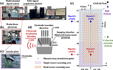
Figure 3. Schematic diagram of the phased array transducer -based ABI experimental platform. (a) Overall system diagram. (b) Local enlargement diagram of signal source and ultrasound irradiation region. (c) Local enlargement diagram of acrylic plate and phantom region. (d) Schematic diagram of electrode direction and ultrasound incidence direction. (e) Schematic of acoustic field raster scanning. (f) Phantom physical image.
Download figure:
Standard image High-resolution imageThe electrodes used in the study are platinum wire electrodes with a length of 15 mm and a diameter of 0.5 mm, which are soldered and connected to the internal signal wires of the BNC, and each pair of dipoles generates sinusoidal signals with the same frequency, equal amplitude, and opposite phase to simulate neuronal discharge process based on a multi-channel signal generator. The electrode tip is located in the y = 0 cross-section and the ultrasound is incident along the z-axis through the open side of the imaging chamber (figure 3(d)). The dipole, acquisition electrode, reference electrode and ground electrode setting positions for the experiment are shown in table 2, where Dipole1+ is set at (57, 0) and Dipole2+ is set at (60, 0).
Table 2. Electrode excitation parameters and positions.
| Frequency (Hz) | Amplitude (mV) | Phase (°) | Location (mm) | Schematic color | |
|---|---|---|---|---|---|
| Dipole1+ | 8 | 20 | 0 | (57, 0) | Red |
| Dipole1− | 8 | 20 | 180 | (57, −9) | Red |
| Dipole2+ | 13 | 20 | 0 | (60, 0) | Blue |
| Dipole2− | 13 | 20 | 180 | (60, −9) | Blue |
| Collection | — | — | — | (58.4, 9) | Green |
| Reference | — | — | — | (68.4, 9) | Purple |
| Grounding | — | — | — | (78.4, 9) | Black |
3.2.2. ABI experimental methods
Each electrode was inserted into the y = 0 section in the phantom along the y-axis direction according to the set position, where the phantom is composed of acrylamide (AM), ammonium persulfate (APS), N, N'-methylenebisacrylamide (MBA), and N, N, N', N'-tetramethylethylenediamine (TEMED), egg white solution, and physiological saline [10, 28].
For the single-source experiments in Dipole1+, the transducer was modulated to perform a  raster scan of the y = 0 cross-section in 0.2 mm steps using the array modulation method in 2.1.2 at an initial excitation voltage of 5 V for each array (purple area in figure 3(e)). For double-source experiments in Dipole1+ and Dipole2+,
  raster scans were performed in 0.2 mm steps (yellow area of figure 3(e)). Pure water single-source phantom experiments, transcranial single-source phantom experiments, and transcranial double-source phantom experiments were performed. The voltage signals generated by the dipole electrodes were acquired, amplified and filtered by the SynAmps2 system (Neuroscan Curry 9, USA) with a sampling rate of 20 kHz, an acquisition time of 20 s for each point, and a bandpass filtering range of 0–3500 Hz.
3.2.3. Signal acquisition and processing methods
The voltage signals acquired by SynAmps2 during ultrasonic irradiation of each target point were used as raw data, and the raw data were pre-processed by removing 50 Hz industrial frequency interference and downsampling from 20 kHz to 4 kHz. The pre-processed data were band-pass filtered at ultrasound pulse repetition frequency (PRF) ± 50 Hz to preserve the high-frequency signal at the 500 Hz. The 20 s envelope signal data was selected and divided into 20 segments of data at 1 s intervals, the data was wave-aligned, superimposed and averaged to obtain the 1 s envelope signal, which is the decoded signal of the ultrasonic irradiation point. The peak average value of the decoded signal was taken as the AE signal amplitude at that ultrasound irradiation point, and the AE signal values obtained at each point during the ultrasound raster scan were used to plot the dipole localization map.
4. Results
The modulated focused acoustic field distributions were first analyzed under both pure water and transcranial conditions, and then single-source and double-source ABI were tested based on the multi-array phased array transducer.
4.1. Phased array transducer transcranial focused acoustic field results
4.1.1. Array excitation signal modulation
Figure 4 shows a schematic of array calibration, transcranial geometric focusing, and offset geometric focusing array delays. Figure 4(a) shows the geometrically focused acoustic pressure of each array under different excitation conditions. Figure 4(b) shows a schematic diagram of the transcranial geometric focusing array delay, where the black line is the delay curve of each array after modulation by the method of 2.1.2, and the red line is the delay curve of each array element of the self-focusing method without any modulation. Figure 4(c) shows a schematic diagram of the delay of the transcranially modulated offset focusing arrays, where the black, blue, green and orange lines are the delay curves of each array at the four focal points of (0,0,60), (0,0,59), (0,0,58), and (0,0,57), respectively, after modulation by the method of 2.1.2.

Figure 4. Schematic of array calibration, transcranial geometric focusing, and offset geometric focusing array delays. (a) Geometric focus acoustic pressure plots of each array individually excited at excitation voltages of 2 V, 5 V, 8 V, respectively. (b) Transcranial geometric focusing. (c) Transcranial offset geometric focusing.
Download figure:
Standard image High-resolution imageAs can be seen from figure 4(a), the average values of acoustic pressure at the geometric focus of each array are 7.8 kPa, 17.95 kPa, and 22.52 kPa for excitation voltages of 2 V, 5 V, and 8 V, respectively, with a good output consistency. As can be seen from figure 4(b), the initial delay of each array after modulation varies, with the earliest excitation of array No. 111, which has an initial delay of 0 ns, and the latest excitation of array No. 52, which has an initial delay of 1590 ns; the initial delays of each array without modulation are all 0 ns. As can be seen from figure 4(c), the initial delays of each array after modulation are all different, when the preset focuses are (0,0,60), (0,0,59), (0,0,58) and (0,0,57), in which the No. 52 array are all the latest excitation, and the initial delays of the No. 52 array at each focus are 1590 ns, 1400 ns, 1210 ns and 990 ns, respectively; the No. 111 array are all the earliest excitation, and its initial delay is 0 ns.
Figure 5 shows the results of the transcranial modulation numerical simulation. Figure 5(a) shows the set focal point (0, 0, 57). Figure 5(b) shows the set focal point (0, 0, 58); figure 5(c) shows the set focal point (0, 0, 59). Figure 5(d) shows the set focal point (0, 0, 60). As can be seen from figure 5, the acoustic pressure field after modulation under numerical simulation conditions can be focused at the set position, and the focal acoustic pressure is 0.49 MPa.

Figure 5. Numerical simulation results of transcranial modulation. (a) Setting the focal point (0, 0, 57). (b) Setting the focal point (0, 0, 58). (c) Setting the focal point (0, 0, 59). (d) Setting the focal point (0, 0, 60).
Download figure:
Standard image High-resolution image4.1.2. Focused acoustic field comparison
The results of the comparison of transcranial self-focusing and modulated focusing at the geometric focus are shown in figure 6, where figure 6(a) shows the self-focusing acoustic pressure field, figure 6(b) shows the modulated focusing acoustic pressure field, figure 6(c) shows the self-focusing −6 dB focal area, figure 6(d) shows the modulated focusing −6 dB focal area, figure 6(e) shows the contrast of the focusing field contours, and figure 6(f) shows the contrast of the acoustic axial sound pressure curves. From figures 6(a) and (b), the maximum acoustic pressure is 0.18 MPa for self-focusing and 0.46 MPa for modulated focusing. The modulated acoustic pressure was increased by a factor of 1.56. From figures 6(c)–(e), it can be seen that the area of the self-focusing focal domain is 4.09 mm2 and there is a large parafocal flap; after modulation of focusing, the focal domain is 2.64 mm in the long axis and 0.83 mm in the short axis, with an area of 1.65 mm2 and basically no parafocal flap. The focal domain area was reduced by 59.66% after modulation. From figure 5(f), it can be seen that the focus of self-focusing exists about 1 mm forward; the focus of modulated focusing is accurately focused at the preset (0, 0, 60), and the effect of modulated focusing is obviously better than self-focusing.
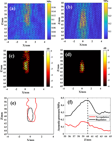
Figure 6. Comparison of focusing results under self-focusing and modulation at the geometric focus. (a) Self-focusing acoustic pressure field. (b) Modulated focused acoustic pressure field. (c) Self-focusing −6 dB focal area. (d) Modulated focus −6 dB focal area. (e) Comparison of focal area contours. (f) Comparison of acoustic pressure curves of acoustic axis.
Download figure:
Standard image High-resolution imageUnder the conditions of setting the focus as (0,0,60), (0,0,59), (0,0,58), and (0,0,57), the modulated focusing results are shown in figure 7, where figures 7(a)–(d) show the focused acoustic pressure fields when different focuses are set, and figures 7(e)–(h) show the corresponding attenuated −6 dB focusing fields, respectively. From figures 7(a)–(d), it can be seen that the maximum pressure of the acoustic field at the geometrical focal point for focusing and −Z direction shifted forward by 1 mm, 2 mm, and 3 mm are 0.46 MPa, 0.53 MPa, 0.55 MPa, and 0.50 MPa, respectively. From figures 7(e)–(h), the focal domain areas at each point are 1.65 mm2, 1.62 mm2, 1.25 mm2 and 1.51 mm2, respectively.

Figure 7. Map of the results of modulation focusing. (a)–(d) Focused acoustic pressure fields when the set focus is (0,0,60), (0,0,59), (0,0,58), and (0,0,57), respectively; (e)–(h) corresponding attenuation of −6 dB focal domain.
Download figure:
Standard image High-resolution imageThe focal domain contour and the acoustic axis pressure curve of the modulated offset focus are shown in figure 8, where figure 8(a) shows the focal domain contour and figure 8(b) shows the acoustic axis pressure curve. As can be seen from figure 8, the regulated focus is basically focused at the preset focus, realizing a regulated offset focus of 3 mm.

Figure 8. Focal area contours and acoustic axis pressure curves for acoustic axis direction modulation. (a) Focal domain contour. (b) Acoustic axis pressure curves.
Download figure:
Standard image High-resolution image4.2. ABI results based on phased array transducer
4.2.1. Single dipole source
4.2.1.1. Localization
The voltage signals acquired under the conditions of setting the phased array excitation voltage of 5 V, the Dipole1 discharge frequency of 8 Hz and the set position of (57, 0) are shown in figure 9, in which figure 9(a) shows the voltage time-domain signals with/without ultrasonic irradiation, and blue line is the signal with ultrasonic irradiation, and orange line is the signal without ultrasonic irradiation; figure 9(b) shows the spectrograms of the low-frequency bands of the two parts; and figure 9(c) shows the high-frequency bands of the spectrograms at the PRF of the two parts. As can be seen in figure 9(a), the time-domain signals of the voltages collected with/without ultrasonic irradiation are basically the same, and there is a high-frequency spike 'burr' in the time-domain signals with ultrasonic irradiation (black arrows zoom). As can be seen from figure 9(b), the spectrograms of the low-frequency bands with and without ultrasonic irradiation are basically the same for both conditions, and both are dominated by 8 Hz. As can be seen in figure 9(c), the acquired signal without ultrasonic irradiation has no specific frequency in the high-frequency band, and the acquired signal with ultrasonic irradiation contains the PRF of ultrasound (500 Hz).
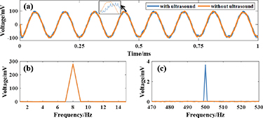
Figure 9. Time-domain and frequency-domain plots of the original acquired signals. (a) Comparison of voltage time-domain signals with/without ultrasonic irradiation. (b) Spectrogram of the low frequency band 1–15 Hz with/without ultrasonic irradiation. (c) Spectrogram of the high-frequency band 470–530 Hz with/without ultrasonic irradiation.
Download figure:
Standard image High-resolution imageFigure 10 shows the results of dipole localization in the phantom via pure water and simulated skull under the above conditions, respectively, where figures 10(a) and (b) shows the results of dipole localization under pure water; figures 10(c) and (d) shows the results of dipole localization under simulated skull. As can be seen from figures 10(a) and (b), the maximum value of the AE signal in the pure water experiment is 725.31 μV, which locates the Dipole1+ position at (0, 56.8), and the z-direction error is 0.2 mm compared with the set position. As can be seen from figures 10(c) and (d), the maximum value of the AE signal in the simulated skull experiment is 134.22 μV, which localizes the Dipole1+ position at (0, 56.6), and the z-direction error is 0.4 mm compared to the set position. As expressed in equation (7) in section 2.2.2, the AE signal is directly related to the focal acoustic pressure. The AE signal was reduced by 81.49% due to the presence of the simulated skull.
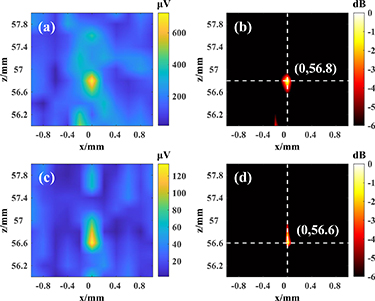
Figure 10. Localization result maps of single source dipole. (a) Localization imaging map of the AE signal under pure water. (b) Localization imaging decay thermogram under pure water. (c) Localization imaging map of the AE signal under simulated skull. (d) Localization imaging decay thermogram under simulated skull.
Download figure:
Standard image High-resolution image4.2.1.2. Decoding
The acquired single dipole source voltage signal is processed by the decoding algorithm of 3.2.3 and the decoded signal is obtained as shown in figure 11, in which figure 11(a) shows the comparison between the decoded signal and the source signal under pure water, with the blue curve being the decoded signal and the orange curve being the source signal; figure 11(b) is the spectrogram of the experimental decoded signal under pure water experiment; figure 11(c) is the comparison of the decoded signal and the source signal of the under simulated skull; and figure 11(d) is the spectrogram of the experimental decoded signal of the under simulated skull experiment. Calculations from the data in figures 11(a) and (b) show that the Pearson correlation coefficients of the decoded signal and source signal of Dipole1+ under pure water and simulated skull experiments are 0.94 and 0.93, respectively.
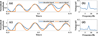
Figure 11. Decoding map of single dipole source signal. (a) Comparison map of decoded signal and source signal under pure water. (b) Spectrogram of decoded signal under pure water. (c) Comparison of decoded signal and source signal under simulated skull. (d) Spectrogram of the decoded signal under simulated skull.
Download figure:
Standard image High-resolution image4.2.2. Double dipole source
4.2.2.1. Localization
Under the conditions of setting the phased array excitation voltage of 5 V, Dipole1+/Dipole2+ positions of (0, 57)/(0, 60) and discharge frequencies of 8 Hz/13 Hz, the localization results of the simulated skull experiments are shown in figure 12, in which figure 12(a) is the localization imaging map of the AE signal; and figure 12(b) is the localization imaging attenuation thermogram. From figure 12(a), the maximum value of AE signal near Dipole1+ is 186.66 μV; the maximum value of AE signal near Dipole2+ is 236.18 μV. From figure 12(b), it can be seen that the position of localized Dipole1+ is at (0, 57.2), and the z-direction error in the simulated skull experiment is 0.2 mm compared with the set position; the position of localized Dipole2+ is at (−0.2, 60), and the x-direction error in the simulated skull experiment is 0.2 mm compared with the set position.

Figure 12. Maps of localization results of dual-source dipoles under simulated skull. (a) Localization imaging map of AE signal under simulated skull. (b) Localization imaging attenuation thermogram under simulated skull.
Download figure:
Standard image High-resolution image4.2.2.2. Decoding
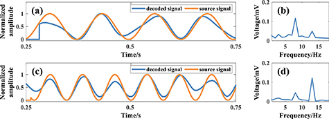
The acquired double dipole source voltage signals are processed by the 3.2.3 decoding algorithm and the decoded signals are shown in figure 13, in which figures 13(a) and (c) are the comparison maps of the decoded signals and source signals of Dipole1+ and Dipole2+ by the simulated skull experiments, the blue curve is the decoded signals, and the orange curve is the source signals; and figures 13(b) and (d) are the spectral maps of the decoded signals of Dipole1+ and Dipole2+ by the simulated skull experiments, respectively. The Pearson correlation coefficients between the Dipole1+/Dipole2+ decoded signal and the source signal in the simulated skull experiment can be calculated from the data in figures 13(a)–(d) to be 0.90 and 0.89, respectively.
Figure 13. Maps of decoding results of dual-source dipoles under simulated cranial. (a) Comparison map of Dipole1+ decoded signal and source signal. (b) Spectrogram of Dipole1+ decoded signal. (c) Comparison map of Dipole2+ decoded signal and source signal. (d) Spectrogram of Dipole2+ decoded signal.
Download figure:
Standard image High-resolution image
5. Discussion
In this paper, based on ABI under the effect of focused pulsed ultrasound with an excitation voltage of 5 V at the array, a center frequency of 1.1 MHz and a PRF of 500 Hz, we firstly explored the transcranial acoustic field modulation distribution, and further localized and decoded the single-source and dual-source dipole signals. The results of acoustic field modulation showed that the simulation-guided modulation results were significantly better than self-focusing, and precise modulation of intracranial target focusing could be realized. The results of single-source experiments show that this study can accurately localize the source signal position with mm-level spatial resolution, the transcranial localization error is less than 0.4 mm, and the decoding accuracy is greater than 0.93; the results of dual-source experiments show that the transcranial localization error is less than 0.2 mm, and the decoding accuracy is greater than 0.89.
In this study, it is found that there will be unavoidable errors between experimental and numerical simulations, which may be due to the mismatch between simulation parameters and real parameters. A homogeneous acrylic plate is used here to simulate the human skull (mainly cortical bone), ignoring the trabecular bone structure. The smooth and ideally homogeneous acrylic plate may not fully reproduce the problems of scattering and acoustic field distortion caused by the heterogeneous structure of the real skull, which is different from the actual situation. We have proposed corresponding modulation methods for phase modulation, amplitude modulation and distance compensation of the arrays in our previous study. To address the problem of acoustic field aberrations caused by strong acoustic attenuation and cranial heterogeneity [29]. And we will analyze the differences between the simulation and the experiment based on more real animal and volunteer cranial data in the later study to achieve more accurate transcranial acoustic field modulation.
In addition, we investigated dipole discharges at 8 Hz and 13 Hz based on the discharge frequencies of  and
and  rhythm in EEG. In this paper, the amplitude of the source signal is set to 20 mV based on the signal generator, which is larger than the real EEG signal amplitude, and the localization and decoding effects after reducing the amplitude need to be further investigated. The present study was performed only with the set conditions of the focused pulse wave described above, and the effects of FUS parameters on neuronal localization and decoding will be investigated in the next step. This paper is based on the SynAmps2 system commonly used for signal acquisition in normal EEG acquisition (<100 Hz), which may degrade the signal-to-noise ratio of high-frequency signals when acquiring signals, and high-frequency acquisition devices specifically designed for acquiring AE signals are likewise worthy of in-depth study.
6. Conclusions
In this study, we explored the effect of transcranial acoustic field modulation and the effect of dipole localization and decoding based on simulated skull, phantom experiments and numerical simulation of focused ultrasound. The results show that accurate transcranial acoustic field modulation focusing, high-precision localization of the source signal position and decoding of the source signal waveform can be achieved. We expect to solve the problem of cranial bone affecting the effect of ABI from the origin based on multi-array ultrasonic phased array, and the related research results provide a new approach to localize neurons and epileptic focus by ABI.
Acknowledgments
This research was supported by the National Natural Science Foundation of China (Nos. 62122059, 81925020, 61976152). Introduce Innovative Teams of 2021 'New High School 20 Items' Project (2021GXRC071). Research Program Project of Tianjin Municipal Education Commission (2022KJ198).
Data availability statement
All data that support the findings of this study are included within the article (and any supplementary files).