

Abstract
Summertime internal melting of Antarctic sea ice is common due to the penetration of solar radiation below the snow and ice surface. We focus on the role of internal melting and heat conduction in generating gap layers within the ice. These often occur approximately 0.1 m below the ice surface. In a small-scale survey over land-fast sea ice in Prydz Bay, East Antarctica, we observed, for the first time, gap layers 0.6–1.0 m below the surface for both first-year ice and multi-year ice. A 1D snow/ice thermodynamic model successfully simulated snow and ice mass balance and the evolution of the gap layers. Their spatial distribution was largely controlled by snow thickness and ice thickness. A C-shaped ice temperature profile with the lowest values in the middle of the ice layer resulted in heat flux convergence causing downward progression of the internal melt layer. Multidecadal (1979–2019) seasonal simulations showed decreasing air temperature favored a postposed internal melting onset, reduced total internal melt, and delayed potential ice breakup, which indicated a higher chance for local coastal ice to be shifted from first-year ice to multi-year ice.
Export citation and abstract BibTeX RIS

Original content from this work may be used under the terms of the Creative Commons Attribution 4.0 license. Any further distribution of this work must maintain attribution to the author(s) and the title of the work, journal citation and DOI.
1. Introduction
Summer sea ice in Antarctica is characterized by a common occurrence of 'gap layers', which consist of deteriorated sea ice of extremely high porosity, often characterized by honeycomb-like ice structures filled with water, slush, as well as algal and microbial community (Kattner et al 2004, Ackley et al 2008, Norman et al 2011). Gap layers are most common in old first-year or multi-year sea ice, and have typical thicknesses of 0.04–0.12 m (Fritsen et al 2001, Haas et al 2001). Gap layers are rare in the Arctic, where the strong summer melt typically results in the removal of the snow cover and the formation of surface melt ponds (Rösel et al 2012) instead of gap layers.
Gap layers are important for both sea ice mass balance and biological activity. According to Ackley et al (2008), sea ice melt rates related to gap layer formation typically range from 0.1 to 0.75 cm d−1, which accumulate to 0.02–0.22 m during the short (20–30 days) melt period in Antarctic summer. During autumn and winter, refreezing of gap layers and surface slush may contribute to even half of ice formation in the western Weddell Sea (Lytle and Ackley 1996). By providing suitable light, liquid water and salinity conditions, gap layers are ideal for biological productivity and, if the layers are widespread, they are suggested to strongly contribute to sea-ice related biological production in Antarctica (Underwood et al 2010, Vancoppenolle et al 2010, Nomura et al 2018, Selz et al 2018).
Different formation mechanisms of gap layers have been suggested. Ackley et al (1979) and Ackley and Sullivan (1994) stressed the importance of dark algal material in absorbing solar radiation, which results in sub-surface melting and gap layer formation, which further enhances algal growth, generating a positive physical-biological feedback loop. In summer the strong solar radiation penetrates below the ice surface and creates internal melting (Liston and Winther 2005). The gap layer formation mechanisms proposed by Fritsen et al (1998) and Haas et al (2001) were based on granular ice formation due to refreezing. Fritsen et al (1998) addressed the flooding of sea ice under a heavy snow cover and partial refreezing of the flooded layers, which allows the drainage of salt from the refrozen layer to the gap layer below, which does not entirely refreeze but remains as slush. This process occurs usually in pack ice, where there is open water nearby in leads, and rarely in landfast ice, except possibly to a small extent near tide cracks. Haas et al (2001) focused on the role of superimposed ice formation when snowmelt results in the percolation of meltwater to the snow-ice interphase, where the water refreezes forming a fresher ice layer. Ackley et al (2008) addressed the role of heat conduction in summertime conditions with a downward heat flux from the snow pack to sea ice. In such conditions, temperature increases in the upper parts of sea ice and the salinity decreases through brine drainage. In these upper layers with low salinity, heat is conducted downward without generating melt, but melt occurs in the saline gap layer. Hence, a gap layer can be generated without biological activity and superimposed ice/snow-ice formation, as long as there is a downward conductive heat flux in snow and upper ice layers. Observations and modeling of the gap layer are challenging and have great importance for the understanding of sea ice structure and processes since the gap layer is one of the components of multiphase sea ice (Hunke et al 2011).
In this paper, we focus on gap layers in the Antarctic landfast sea ice, which in summer comprises 35% of the overall Antarctic sea-ice area (Fraser et al 2012). As landfast ice is immobile, thermodynamic processes dominate ice evolution until its breakup (Heil et al 1996, Yang et al 2015, Zhao et al 2019b). Combining in situ observations and a snow/ice thermodynamic model, we investigate factors contributing to gap layer formation. We go beyond the previous studies by simulating the roles of both heat conduction and absorption of solar radiation in snow and ice and their contributions to the gap layer formation. The model results are quantitatively compared with observations. The modeling experiments cover time scales from seasonal to multi-decadal.
2. Data and methods
In Prydz Bay, observations of land-fast ice have been carried out in the coastal area near both Chinese Zhongshan and Russian Progress Research Stations (Zhao et al 2019a). Applying newly released field data allows us to map and discover gap layer distribution at different depths below the ice surface (figure 1). Unlike in Ackley et al (2008), we observed gap layers, for the first time, at depths of 0.6–1.0 m below the ice surface. The detailed observations are summarized in table S1.
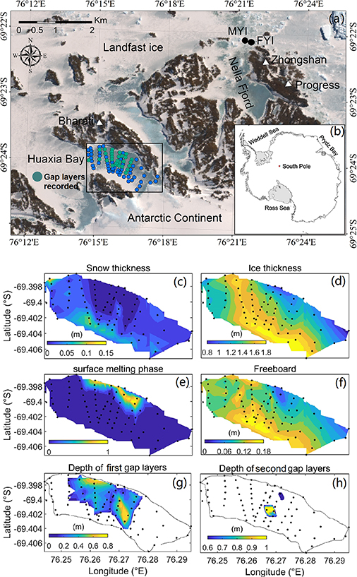
Figure 1. Small-scale landfast sea ice observations carried out during 29th CHINARE program on 11–13 December 2012 in the vicinity of Indian Bharati Station in Prydz Bay, about 10 km west of the Chinese Zhongshan and Russian Progress stations. (a) A map of the study region and distribution of the 79 measurement sites. The green circles indicate the locations where gap layers were detected. The background is a Landsat image (15 m resolution) from 30 November 2012. (b) The Prydz Bay study region, denoted by a black box, within the Antarctic. 2D maps of (c) snow thickness; (d) ice thickness; (e) surface melting phase (0: dry surface; 1: melting surface); (f) ice freeboard; (g) the depth of the first gap layers; (h) the depth of the second gap layers. The depth of the gap layer is defined as the distance of the top of the gap layer from the ice surface.
Download figure:
Standard image High-resolution imageA 1D high‐resolution Thermodynamic Sea Ice and snow model (HIGHTSI) (Launiainen and Cheng 1998) was used to simulate snow and ice temperatures and mass balance, affected by surface, internal and basal melt, as well as snow-to-ice transformation. The vertical distribution of solar radiation absorbed below snow or ice surface was calculated according to Grenfell and Maykut (1977) and Perovich (1996). The absorbed solar radiation contributed to both the heat balance of the surface layer and the warming of the internal snow and ice. This parameterization allows HIGHTSI to quantitatively simulate the sub-surface melting of snow and ice (Cheng et al 2003). HIGHTSI has been extensively validated and widely applied in both process studies (Cheng et al 2008, 2013, Wang et al 2015, Merkouriadi et al 2017, 2020, Mäkynen et al 2020) and operational service for the Prydz Bay region (Zhao et al 2020). Detailed model parameterizations are given in the supporting file (table S2).
The HIGHTSI control run covers the entire melting season from late spring (1 November 2011) until early autumn (31 March 2012). The initial snow and ice thicknesses were 0.17 m and 1.5 m, respectively, based on manual in situ observations near the Russian Progress station. Those measurements were made on a weekly basis between December 2011 and January 2012. The accuracy of the measurements was 0.01 m. Those routine measurements were compared with HIGHTSI results. The initial temperature profile in snow and ice was assumed as a piecewise linear distribution (Lei et al 2010). The meteorological parameters, used as model forcing, were observed by an automatic weather station at the Chinese Zhongshan Station (figure 1). The wind speed (Va), air temperature (Ta), and relative humidity (Rh) were observed at 10 m height with a 1 min time interval. The total cloud fraction (CN) was observed visually four times daily. Total precipitation (Prec) was observed at the Russian Progress Station, 1 km southeast of Zhongshan Station. On the basis of previous studies at near-coastal sites in Prydz Bay, the oceanic heat flux (Fw) has an annual cycle with a maximum value in March and a minimum in September (Heil et al 1996, Lei et al 2010). Unfortunately, no summer observations were available due to unsafe ice conditions. We, therefore, assumed a simple linear increase of monthly mean oceanic heat flux from an observed 16 W m−2 in November to an observed 32 W m−2 in March (Zhao et al 2019a). Figure S2 shows the time series of weather data and oceanic heat flux used for the HIGHTSI run.
A recent study found large temporal and spatial variations of air temperature in the margins of East Antarctica (Wei et al 2019), while air temperature has a profound impact on landfast ice formation (Li et al 2020). To investigate the long-term impact of air temperature on internal ice melting, we carried out multidecadal (1979–2019) seasonal simulations using ECMWF Reanalysis ERA-Interim from the European Centre for Medium-Range Weather Forecasts as forcing. The selection of ERA data was justified because ERA-Interim had the best skill scores among five atmospheric reanalysis data sets over the Antarctic Sea ice (Jonassen et al 2019). For each melting season during 1979–2019, the simulation started on 1 November and ended on 31 March using the same initial snow and ice thickness as in the control run.
3. Results
3.1. Mapping gap layers
Gap layers existed extensively during observations occurring at 37% of the measurement sites (figure 1(b)). The depths of gap layers ranged from 0.05 to 1.0 m below the ice surface. The gap layers were found in locations that were snow-free or where the snow pack was thin. In several locations where gap layers were deep, statistically 0.4–0.8 cm below the surface, the surface was melting. The study domain was covered by level ice with thickness ranging from 0.76 to 1.93 m. The ice freeboard correlated with the ice thickness (correlation coefficient 0.62), and no surface flooding was observed, even close to tide cracks between icebergs and islands. This suggested that the gap layers were unlikely caused by ice raft, deformation, or snow flooding. The details of the gap layers are summarized in table S1. For the first time, two-gap layers were discovered in a single borehole at several locations, where the first gap layer was 0.05–0.4 m below the ice surface and the second gap layer was farther down, 0.6–1.0 m below the ice surface (figure S1).
3.2. Snow and ice mass balance and internal ice melting
During the simulation period, the observed mean air temperature was −3.9 ± 4.1 °C with the highest monthly means observed in December (1.7 ± 2.9 °C) and January (−0.6 ± 1.8 °C). The air temperatures were sufficiently high for the melt of most of the snow pack, but there was no direct surface melt of ice, as some snow remained on top of ice during the entire study period. Hence, the ice melt was due to (a) solar radiation that penetrated through the snow and (b) the oceanic heat flux beneath the ice column.
The simulated snow and ice evolutions were well in agreement with the observations (figure 2(a)). The mean biases for simulated snow and ice thickness from the HIGHTSI model were −0.008 ± 0.029 m and −0.005 ± 0.022 m, respectively. The modeled internal ice melting occurred initially on 20 December at a depth of 0.07 m below the ice surface. This isothermal layer gradually moved downward with a mean rate of 1.2 × 10⁻² m d−1, and by 29 January it had become deeper, down to a depth of 0.67 m. By mid-February, the internal ice melting stopped although the ice layer was still melting from the bottom. In mid-March, the ice melting stopped, and the freezing season started. In reality, landfast sea ice may start to disintegrate in February due to impact of wind and ocean current. This sea ice dynamics was not considered in our modeling. The calculated snow thickness and ice thickness are the thermodynamic results. The modeled total sea ice melt rate was 2.6 × 10⁻³ m d−1 during the observation available period of November and December, which was close to the observed ice melt rate of 2.2 × 10⁻³ m d−1. During the entire simulation period, internal melt lasted for 56 days, with a mean rate of internal melt of 2.8 × 10⁻³ m d−1 and the total ice melt was 0.94 m, of which 0.16 m (17%) was internal melt, which agrees with the internal melt rates of 1.0–7.5 × 10⁻³m d−1 and amount estimate of 0.02–0.22 m by Ackley et al (2008). If turning off the internal melting parameterization in the control run, it yielded a total ice melt of 0.83 m, which is some 12% smaller than in the model run considering internal melting.

Figure 2. (a) The time series of snow and ice thickness, snow/ice temperature as well as the occurrence and depth of internal ice melt layers (white regions); the zero location represents the snow/ice interface; the (*) and (o) are observed snow and ice thickness, respectively, before the ice was eroded and not safe for on-ice measurement. (b) The distribution of solar radiation within snow and sea ice; (c) the distribution of conductive heat flux within snow and ice. The subplot (d) shows the instantaneous profiles of (a)–(c) (vertical black lines) on 1 January. In (c), the positive values represent downward fluxes, and the negative ones represent upward fluxes. The isolines of zero values are marked by solid gray lines.
Download figure:
Standard image High-resolution imageWhen a deep snow pack is present, the penetrating solar radiation is confined to its upper part (figure 2(b)), because the extinction coefficient of snow is large. When the snow pack gets thinner, solar radiation penetrates through it and deeper into sea ice, because the extinction coefficient of sea ice is much smaller (Perovich 1996). In early November, the air temperature and downward solar radiative flux started to increase gradually and heat the snow pack and upper ice layers. In the lower parts of the ice layer, the conductive heat flux (figure 2(c)) was upward in November but then decreased in magnitude and turned downward in mid-January. The initial linear in-ice temperature profile turned to a nonlinear one by the second half of November, and further to practically isothermal conditions by late December. For a given time step (figure 2(d)), the larger gain of solar radiation at the top ice layer increased the ice temperature and generated a downward heat flux in the upper half of the ice layer, while the continuous heat flux from the warm ocean to the ice bottom increased ice temperature and generated an upward conductive heat flux in the lower half of the ice layer. These fluxes converged in the middle of the ice layer and resulted in ice melt generating the gap layer.
The evolution of internal melting was revealed by the control run. However, it is difficult to directly compare the model results with the small-scale survey. We, therefore, performed a group of model experiments for the same period using the same external forcing but different initial snow thickness and ice thickness. Furthermore, clouds have a large impact on the downward shortwave and longwave radiation (Lachlan-Cope 2010), which affect the surface energy balance and internal melting. As the cloud fraction was observed only four times a day, its time series includes uncertainty, which may cause modeling errors in the ice melt and development of the gap layer. To investigate the sensitivity of the total internal ice melt, maximum depth of internal melt, and the onset date of internal melt to the cloud fraction and the initial snow and ice thickness, we ran a group of model experiments. To investigate the sensitivity to total cloud fraction, the initial snow and ice conditions were set the same as in the control run. To investigate the sensitivity to the initial snow thickness, the initial ice thickness and time series of cloud fraction were set the same as in the control run. To investigate the sensitivity to initial ice thickness, the snow thickness and the time series of the cloud fraction were the same as in the control run. To investigate the sensitivity to total cloud fraction, the initial snow and ice conditions were set the same as in the control run (table S3).
The probability density distribution (PDF) of modeled internal melting depth during entire December was compared with the survey observations (figure 3(a)). Both observed and modeled gap layer depths followed a Gaussian distribution. For the gap layer between 0.3 m and 0.5 m, the modeled and observed PDF of the gap layer depth were close to each other, indicating that the evolution of internal melting and the gap layer can be realistically modeled.

Figure 3. (a) Statistical comparison between modeled and observed depth of the gap layers in December. (b) Sensitivity of the total internal ice melt (black line); maximum depth of internal ice melt (red line) and the onset date of internal ice melt (blue) to the initial snow thickness. (c) Sensitivity of the same parameters to the initial ice thickness, and (d) sensitivity of the same parameters to cloud fraction.
Download figure:
Standard image High-resolution imageA deeper initial snow pack effectively reduces both the total amount and maximum depth of internal melt (figure 3(b)). These effects are due to the large extinction coefficient and high surface albedo of snow. Most of solar radiation is either reflected back to air or used to heat the snow surface and the layers slightly below it. The onset of internal melt is considerably delayed when the snow pack is deep. This is because thicker snow needs more time to melt and sublimate before bare ice can absorb more shortwave radiation flux and penetrate further into sea ice interior. Model sensitivity runs indicated that the onset of snow-free conditions is linearly delayed by up to a month when the initial snow thickness increases from 0.1 to 0.7 m.
In lieu of snow, increasing initial ice thickness increases the total amount and maximum depth of internal ice melting (figure 3(c)). During the period of internal melting, the ice layer is almost isothermal, and the internal melt penetrates through most of the ice layer. Hence, the thicker the ice is, the more ice is available to melt. Increasing ice thickness only causes a small delay in the onset of internal melt. This is because the temperature increase in the upper ice layers is mostly due to solar radiation (not affected by the amount of ice below the melt layer) and the contribution of the conductive heat flux is minor.
When cloud fraction increased from 0 to 1, the maximum depth of internal melting showed a nonlinear decrease, reduced by 33% from 0.73 m to 0.49 m, while the total internal melting showed a nearly linear trend, reduced by 61% from 0.23 m to 0.09 m. The internal melting onset was postponed by a few days (figure 3(d)).
3.3. Inter-annual variation of internal melting
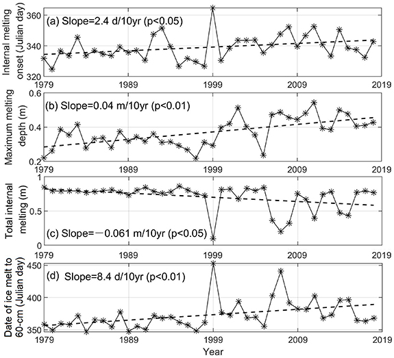
For the multidecadal seasonal simulations driven by the ERA-Interim Reanalysis data during 1979–2019, we pay particular attention to (a) internal melting onset; (b) the maximum internal melting depth, (c) the ratio of internal melting depth to the total ice thickness; and (d) the timing when ice thickness reduced to 60 cm after melting onset. Previous studies have indicated that when the ice thickness reaches this threshold value, the breakup of landfast ice in the Prydz Bay occurs (Lei et al 2010, Yang et al 2015).
The results showed that multidecadal seasonal average snow thickness was between 0.04 and 0.14 m with an average value of 0.07 m (figure S3(b)), in agreement with the early finding of coastal thin snow in the Prydz Bay (Lei et al 2010, Zhao et al 2019b), indicating that ice internal melting easily occurred and developed in this region. The decreasing trend (p < 0.05) of local air temperature (figure S3(a)) postponed internal melting onset 2.4 days per decade (figure 4(a)), and the total amount of internal ice melting was accordingly reduced (figure 4(c)). However, the maximum internal melting depth was deepened (figure 4(b)), probably related to the potential increase of solar radiation, with decreasing cloud fraction (figure S3(d)). After late 1990s, all parameters, in particular the internal melt onset, total amount of internal melting, fraction as well as the date of ice melt to 60 cm showed large interannual variations, which may be largely associated with spatial and temporal variation of snow. The late date for ice meltdown to 60 cm thickness may indirectly suggest that the ice breakup could be delayed, and the coastal landfast sea ice accordingly has a higher chance to be shifted from first-year ice to multi-year ice.
Figure 4. The time series of modeled (a) internal melting onset date, (b) maximum melting depth, (c) total internal melting, (d) date of ice melt to 60 cm thickness during the melting season.
Download figure:
Standard image High-resolution image
4. Discussion and conclusion
We observed and modeled gap layers caused by the internal melting of the Antarctic landfast sea ice. The gap layer may be thin, located a few centimeters below the ice surface, or it may occur in the middle of the ice layer. Our results for shallow gap layers approximately agree with previous studies (Fritsen et al 2001, Haas et al 2001, Ackley et al 2008), which have reported gap layers usually at some 0.2 m below the ice surface. Our results for deep gap layers are novel. According to our model experiments, the deepening of gap layers on multidecadal time scales is very likely associated with decreasing air temperature and cloud fraction during summer.
The results of thermodynamic modeling demonstrated that the key factor for internal melt and gap layer formation was the penetration of solar radiation into the sea ice. Several other factors, including air temperature, clouds, snow thickness, and ice thickness, contributed to determining the melt onset date as well as the total amount and maximum depth of internal melt. Due to the large extinction coefficient and high surface albedo of snow, a deeper snow pack reduces both the total amount and maximum depth of internal ice melt and causes a delay in its onset. In the case of bare ice, increasing ice thickness increases the total amount and maximum depth of internal melt.
Ice color is quantitatively associated with the spectrum of solar radiation reflected from the ice surface and scatters within the ice (Lu et al 2018a). White ice is common in the Antarctic and usually results from formations of superimposed ice or snow ice on the surface (Grenfell 1979). However, in the coastline area of Prydz Bay, katabatic winds were so strong that snow was blown away soon after the precipitation events, and therefore snow-free conditions were often seen, making the ice color more bluish. A piece of bluish ice indicates fewer internal scatterers, such as gas bubbles, and thus has a lower albedo and allows more penetration of light into the ice interior (Perovich 1996, Lu et al 2018b). For blue ice, the modeled maximum depth of internal melting was 0.81 m below the ice surface, which is 21% deeper than in the control run.
Considering the formation of gap layers, Ackley et al (2008) stressed the importance of the ice temperature profile, physical-biological feedbacks, and formation of superimposed ice and snow-ice. Our results demonstrated the importance of air temperature, cloud, snow and ice thickness, which are directly linked with the vertical distribution of solar radiation absorbed within the ice layer. Our results suggest that in summer conditions with strong solar radiation, internal melting and associated formation of gap layers are possible even without physical-biological feedback. We note, however, that our study addressed Antarctic landfast sea ice, whereas Ackley et al (2008) addressed drift ice zone, where the boundary conditions for internal melting may be somewhat different. Considering the importance of the shape of the temperature profile, our model results agree with Ackley et al (2008). In our experiments, the oceanic heat flux at the ice base and the strong solar radiation absorbed in the upper layer of the ice column resulted in a profile shape that led to the convergence of conductive heat flux in the middle of the ice column. It resulted in strong internal melting.
There had not been major progress or breakthrough on gap layer investigations since the study of Ackley et al (2008). At least we are not aware of any gap layer modeling study for the Antarctic sea ice. In this paper, we demonstrated that gap layers can be formed by the internal melting of sea ice. Because of the sparse in situ observations, the optical properties of sea ice and snow were presented as integrated bulk values in our model experiments. Although the model runs reproduced the development of gap layers deep below the ice surface, the exact physical mechanisms responsible for the simultaneous occurrence of two gap layers at different depths in an ice column remain unclear. The brine channel migration and gravity drainage are important micro-scale processes within sea ice (Marchenko and Lishman 2017, Thomas et al 2020), and they may also play considerable roles in formation of deep gap layers. Hence, more field data are needed. For example, observations of the vertical profile of physical properties and microstructure of sea ice could result in a better understanding of the spatial distribution of gap layers and the factors controlling it. The water within the gap layers, as the water within ice ridges, may enhance biological activity and biomass production in the ice (Fernández-Méndez et al 2018). The relevant physical and biological observations are scheduled for a future field campaign under the support of the Chinese National Antarctic Research Expedition and will enable new discoveries of characteristics of land fast sea ice in other parts of the Antarctic (Heil et al 2011, Arndt et al 2020).
Acknowledgments
We thank colleagues at the Progress Station for sharing us with snow and ice thickness observations. The study was supported by the National Natural Science Foundation of China (4211101310, 41876212, and 41922045) and the European Commission H2020 Project Polar Regions in the Earth System (PolarRES, Grant 101003590). Two anonymous reviewers are acknowledged for their very constructive and valuable comments that helped to improve the manuscript significantly.
Data availability statement
The data that support the findings of this study are openly available at the following URL/DOI: http://doi.org/10.5281/zenodo.4556496.
Supplementary data (0.8 MB DOCX)