


Abstract
The 2019/20 winter was extremely warm globally and in the Northern Hemisphere extratropics. The main cause of climate extremes particularly in East Asia, was the extreme positive Arctic Oscillation (AO) event superimposed on steady global warming. The negligible trend in the AO over the preceding 41 years makes it possible to distinguish the roles of AO and global warming in the observed extremes. We estimate and compare contributions to January–March 2020 climate extremes by the AO and global warming represented by local temperature trends using the ERA5 reanalysis data. Based on results from a preliminary study, we estimate the contribution by global warming using linear regression while that by the AO using cubic regression, which is more restrained for the high AO index values than linear. The results show that the temperature extremes were mainly caused by the extreme positive AO event which accounts for approximately 3/4 of the observed temperature anomalies in northern East Asia and 2/3 in eastern East Asia. In southern East Asia, the AO contributes negligibly and positive temperature anomalies are related to global warming and local and regional impacts, particularly extreme sea surface temperature, enhance south-westerlies and local radiative forcing. General conclusion is that the observed strong positive temperature anomalies including extreme anomalies over East Asia could have been achieved only as a combined effect of the extreme positive AO event and global warming. Quantification of the roles of the AO and global warming in climate extremes helps to estimate future anomalies caused by extreme AO events as well as assess uncertainties in climate model projections.
Export citation and abstract BibTeX RIS

Original content from this work may be used under the terms of the Creative Commons Attribution 4.0 license. Any further distribution of this work must maintain attribution to the author(s) and the title of the work, journal citation and DOI.
1. Introduction
The 2019/20 winter was the second warmest winter on 141 year record, with January–March (JFM) 2020 temperature anomaly being +1.15 K for globe and +1.53 K for the Northern Hemisphere against the 1901–2000 climatology (NOAA National Centers for Environmental Information 2020). Recent studies (Lawrence et al 2020, Juzbašić et al 2021) have shown that the winter 2019/20 climate extremes in the Northern extratropics were caused by an extremely positive Arctic Oscillation (AO) event. The AO recognized by Thompson and Wallace (1998), (2000) is a seesaw in sea level pressure (SLP) and geopotential height (GPH) anomalies between the polar region and the middle latitudes. In the lower troposphere, the positive AO phase is associated with the negative SLP and GPH anomalies encompassing the polar region and two stretched centers of the positive anomalies over the North Atlantic and North Pacific in the latitudinal belt 40°–50°N. This pattern provides anomalous westerlies on the northern side of this positive anomaly belt and anomalous easterlies on its southern side. It is atmospheric circulation mode that dominates the wintertime climate over whole Northern Eurasia.
In East Asia, the 2019/20 winter was extremely warm, with observed wintertime temperatures being highest on record in Korea and Japan, with number and intensity of cold surges being anomalously low (figures are available at, https://data.kma.go.kr/climate/cdwv/selectCdwvDmap.do?pgmNo=733). The mechanisms of the AO influence on East Asia temperature ensue from these AO-associated SLP/GPH anomaly patterns (Thompson and Wallace 2000) and were discussed in previous studies (e.g. Thompson and Wallace 2001, Wu et al 2006, Park et al 2011, Park and Ahn 2016). The positive AO polarity associates with weakening of the Siberian High due to the enhanced heat advection with anomalous westerlies over Northern Eurasia, resulting in weakening of the East Asia Winter Monsoon (EAWM) (e.g. Gong et al 2001), reducing of frequency, amplitude, and duration of cold surges (Zhang et al 1997, Jeong and Ho 2005, Park et al 2011, Woo et al 2012, Heo et al 2018), and triggering the positive East Asia temperature anomaly (Gong et al 2001). Also, the positive AO polarity associates with the anomalous heat advection from the ocean with the enhanced easterlies on the southern side of the North Pacific stretched center (e.g. Gong and Wang 2003, Suo et al 2009, Lee et al 2013). Therefore, the described mechanisms suggest that a positive AO event can cause positive temperature anomalies in East Asia that provide the basis for our study focused on assessment of a portion of East Asia JFM 2020 observed positive extreme temperature anomalies caused by the extreme AO event and a portion associated with global warming.
The previous studies of the response to the extreme AO event have been focused on hemispheric or continental scale regions. Particularly, Lawrence et al (2020) analyzes zonal mean temperature anomalies. They show that about two thirds of the zonal mean temperature anomalies in the latitudinal belt 40°–70°N are linearly congruent with the AO index in JFM 2020, with the AO-congruent zonal mean positive temperature anomaly being largely contributed from western and north-eastern Eurasia with contribution from northern North America being negative (Lawrence et al 2020, figure 6). However, the authors note that the quantity may partly be attributed to global warming because it was obtained on non-detrended data. Kryjov (2021) studies the separate linear contributions of the AO and global warming to the December–March 2019/20 mean temperature anomalies over Northern Eurasia, focusing mainly on its western part, and reveals a dominant role of the AO enhanced by the trend components. However, the study has remained uncertainties because both the AO and trend contributions were estimated by linear models whereas some studies have suggested nonlinearity in local-scale temperature trends (e.g. Ribes et al 2016) as well as in the temperature-AO relationships (e.g. Higgins et al 2002, Son et al 2012). Therefore, in this study, the appropriate functions representing the temperature trends and the temperature-AO relationships over East Asia are determined through preliminary studies. Kam et al (2022) show that 36% of December–February 2019/20 mean Northwestern Russia temperature anomaly is linearly congruent with the North Atlantic Oscillation index. However, their result is not applicable to East Asia because the studied region is far distant from East Asia and zonal circulation was not strong in December (the AO index was 0.41).
Changes in weather and climate extremes occur regularly and it is evident that extremes of temperature will rise in the daily and seasonal time scales, and intermittent winter extremes will continue to appear (IPCC 2014). Under these climate change, the Northern Eurasia Future Initiative (NEFI) ultimately seeks to develop a sustainable society by establishing appropriate mitigation and adaptation strategies accordingly through analysis of the changing climate and environment (Groisman et al 2017, Soja and Groisman 2018). Located in the easternmost part of the NEFI domain, East Asia is a densely populated area where extreme climate greatly impacts social and economic status and development. Moreover, regional global warming wintertime manifestations in East Asia are strong and spatially inhomogeneous within the region (e.g. Jiang et al 2004, Ahn et al 2014, Xu et al 2016, Luo et al 2020). Therefore, quantification of the separate contributions of global warming and the AO to the extremes of 2019/20 winter could increase our understanding of the forthcoming temperature extremes in East Asia. This not only provides a broader understanding of temperature extremes in the context of global warming but can also help regional decision makers in strategizing mitigation and adaptation. Along with daily mean temperature, we analyze the AO and global warming contributions to maximum and minimum temperatures.
The purpose of the study is separation and quantification of the AO and global warming contributions to the JFM 2020 temperature extremes in East Asia accounting for possible nonlinearity of the local warming trends and temperature-AO relationships and their spatial inhomogeneity.
This paper is organized as follows. Section 2 describes the datasets and details the methods. Analysis of the 2020 regional climate anomalies and contributions by the AO and global warming are posted in section 3. Discussion is in section 4. Section 5 presents conclusions.
2. Data and methods
2.1. Data
The monthly mean AO index (AOI) used is available from the Climate Prediction Center website at www.cpc.ncep.noaa.gov/products/precip/CWlink/daily_ao_index/ao.shtml (accessed 14 June 2021). It is updated monthly following the technology of Thompson and Wallace (2000) with the use of the 1000 hPa GPH (Z1000) fields poleward of 20°N from NCEP-NCAR Reanalysis-1 (Kalnay et al 1996) and the 1979–2000 basic period. Monthly mean indices are estimated by projecting monthly mean anomalies of Z1000 on the loading pattern that was estimated for the basic period as the first EOF of the year-round monthly mean Z1000 anomalies with respect to the corresponding monthly means weighted by square root of the cosine of latitude. All the AO monthly indices have the same loading pattern, and the published indices are not standardized that implies opportunity for estimation of the seasonal mean AOI values. This study focuses on January–March because the extreme seasonal mean AOI was observed during these months in 2020. It is important to note that the linear trend in the JFM AOI during the 41 year period (1979–2019), preceding the analyzed 2020, was negligible, 0.01 σ/year, with 95% confidence intervals being 0.03 σ/year (figure 1).
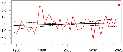
Figure 1. The 1979–2019 time series of JFM AOI and its 41 year linear trend (0.01 σ/year, with 95% confidence intervals being 0.03 σ/year). The AOI value of JFM 2020 is shown with red dot.
Download figure:
Standard image High-resolution imageA reasonable estimate of the contribution of the AO and global warming in East Asia would require high resolution long-term data sets covering up to JFM 2020. We selected the ERA5, a fifth-generation ECMWF reanalysis that covers data from 1979 to the present. The ERA5 reanalysis has a horizontal resolution of 0.25° × 0.25° and 37 vertical levels, it is available from the Copernicus Climate Change Service (C3S) Climate Data Store homepage (https://cds.climate.copernicus.eu/cdsapp#!/search?type=dataset&text=era5). The JFM mean temperature variables we use are seasonal means of daily mean (T2m), maximum (T2max), and minimum (T2min) temperature, obtained based on 1 h data (Hersbach et al 2018). Monthly data are additionally used in supporting analyses: SLP, sea surface temperature (SST), wind at 850 hPa surface, surface net shortwave and long-wave radiation (Hersbach et al 2019a, b). The monthly mean snow cover extent (SCE) data were derived from the Rutgers University Global Snow Laboratory data meshed on the irregular 88 × 88 grid.
2.2. Subregions of East Asia
The local manifestations of global warming as well as the AO impact on temperature essentially differs from each part of East Asia (figure 2). Particularly, the grid-points featuring statistically significant temperature trends are mainly concentrated in the southern part of East Asia and the adjacent seas (figure 2(a)), whereas the AO influence is the strongest in the northern half of the East Asian region (figure 2(b)). Therefore, we divide the whole East Asia region into three subregions allowing more or less spatially homogeneous quantification of the contributions of global warming and the AO to the temperature extremes. Northern East Asia (NEA) is a subregion of comparatively low local temperature trends (LTTs) and of the strongest temperature response to the AO, mainly caused by variations in heat advection associated with the AO. Eastern East Asia (EEA) is a subregion combining both significant temperature trends and strong affect by the AO via its influence on the EAWM. Southern East Asia (SEA) is a subregion of mainly significant LTTs and insignificant correlations of grid-point temperatures with AOI.
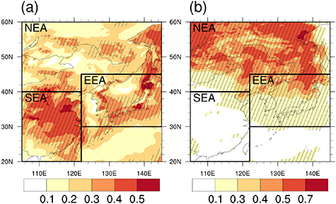
Figure 2. Maps of (a) T2m trends based standardized T2m, and (b) coefficients of determination (R2) between the observed and estimated using cubic regression series of JFM T2m for 1979–2019. Rectangles show selected subregions of East Asia, Northern East Asia (NEA), Eastern East Asia (EEA), Southern East Asia (SEA). Please see details in the text. Thin nets mark the grid-points where (a) the linear trend and (b) correlation coefficient is significant at the 95% confidence level in two-tailed test.
Download figure:
Standard image High-resolution image2.3. Methods
We examined anomalies of the winter 2020 and the contributions of the AO and global warming to these anomalies with respect to climatology from 1979 to 2019. Global warming is characterized by the trend in globally averaged temperature or, that is the same under linear constraint at least, globally averaged LTTs. However, the LTTs, contributing to the global one, essentially differ from each other (e.g. IPCC 2014, figure 1). So that, in our study, a grid-point manifestation of global warming was represented by a 1979–2019 LTT at this grid-point. Our preliminary analysis of the shape of the trend line for three selected subregions of East Asia with the use of linear, quadratic, and cubic polynomial approximations shows that for the analyzed 41 year period the linear approximation is the most appropriate based on F-value assessments. This result is supported by previous studies demonstrated that the non-linear trend with rapid temperature increase in the 1970s and restrained in the 2000s was the result of overlapping the global trends with natural variability, (Meehl et al 2009, Zhou and Tung 2013). Furthermore, Zhou and Tung (2013) showed that linear trend assessments for different recent time intervals within the past 100 years vary insignificantly when overlapping variability was removed. For East Asia, the temperature trend nonlinear approximations underestimate the 2020 temperature value by several tenths of Kelvin as compared with linear for all three temperature characteristics, T2m, T2max, and T2min (figures 3(a)–(c) and S1 (available online at stacks.iop.org/ERL/17/065010/mmedia)). So that, our assessments could be considered as an upper bound of the global warming contribution for East Asia in JFM 2020.
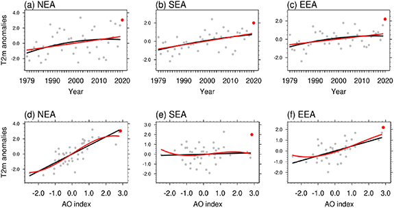
Figure 3. (Top) JFM temperature time series (gray dots) from 1979 to 2019 for T2m for (a) NEA, (b) SEA, and (c) EEA (Unit: K). Linear trend derived on 1979–2019 time series is shown with red line; quadratic trend is shown with black line. The temperature values of JFM 2020 are shown with red dots; (Bottom) Scatterplots showing the temperature-AO relationships (gray dots) from 1979 to 2019 for T2m for (d) NEA, (e) SEA, and (f) EEA (Unit: K). Derived on 1979–2019 time series, cubic relationships are shown with red line, linear relationships are shown with black line. The temperature-AO relationship values of JFM 2020 are shown with red dots.
Download figure:
Standard image High-resolution imageSon et al (2012) documented nonlinearity in the temperature-AOI relationships. For the high and low AOIs some kind of 'saturation' in temperature response occurs that results in overestimation of the temperature values associated with the high and low AOI values under linear constraints. Therefore, we performed preliminary analysis for East Asia and selected the cubic polynomial function as the most appropriate to characterize the temperature-AOI relationships (figures 3(d)–(f) and S2), with cubic regression coefficients being estimated separately for each grid-point.
Since the linear trend in the AOI was negligible in 1979–2019, we consider the AOI and the grid-point linear temperature trend statistically independent during this period (we discuss this assumption in section 4.1). In our study, the LTT and AO contributions are estimated by regression, with the training period being 1979–2019, with 2020 being the target year. For each grid-point we derive a regression equation for the LTT contribution using the grid-point original temperature time series as predictand and time as predictor. Then, we independently derive the cubic regression equation for the AO contribution on the grid-point linearly detrended time series, with the linear trend, although negligible, being subtracted from the AO indices as well. Significance of the regression coefficients was assessed by Student's t-statistic accounting for the effective series size (Bretherton et al 1999). Since regression coefficients may be positive and negative, the appropriate confidence level was set at the 95% in two-tailed tests.
Following recommendations of Wilks (1995, p 311) we assess similarity between the patterns of observed temperature anomalies in JFM 2020 and patterns of the global warming and AO contributions by spatial correlation coefficients. Accuracy of our statistical model is assessed by the root mean squared error (RMSE) between the JFM 2020 observed and estimated temperature fields. We compare the accuracy of representation of the observed temperature field by different estimated fields (the AO, LTT, AO + LTT contributions) by the mean squared skill score (MSSS), recommended by Murphy (1988):

where MSE is the mean squared error of the observed temperature field representation by an estimated field, with the  corresponding to the analyzed estimated field and the
  to the reference one. The MSSS is positive if the analyzed estimated field is closer to the observed one than the reference estimated field.
The statistical significance of the spatial correlation coefficients and MSSS values was assessed using a Monte Carlo resampling approach (Wilks 1995). To account for the spatial correlation structure, we use the moving blocks procedure (Wilks 1997). We estimated p-values by computing 1000 coefficients (MSSS values) between fields of randomly scrambled blocks of observations and unchanged contribution fields. We considered the spatial correlation coefficient (MSSS) significant at the 97.5% confidence level in one-tailed test if the p-value was below 2.5%.
3. Results
3.1. Global analysis of the AO and LTT contributions to T2m anomalies of JFM 2020
As a preliminary analysis to provide a broader understanding of the results for East Asia we examine the AO and LTT contributions to the observed T2m anomalies of JFM 2020 on a global scale. Figure 4(a) shows an exceptionally warm winter in Northern Eurasia (anomalies exceed 5 K), with East Asia anomalies exceeding 2 K, positive anomalies of up to 2 K over south-eastern North America, and negative anomalies of about −3 K over Greenland and Alaska. The AO mainly contributes positively over western (exceeding 5 K) and eastern (up to 5 K) Northern Eurasia and negatively over Greenland (up to −5 K). This spatial pattern of the AO contribution resembles the typical pattern of T2m anomalies associated with the positive AO events, although with stronger anomalies. The contribution of LTT is not spatially uniform. It is the largest over the Eastern Arctic (up to 5 K) while over the continents it is mostly less than 2 K. Areas of the largest underestimation of the JFM 2020 T2m anomalies are Western Siberia (residuals of up to 5 K) and the Labrador Peninsula (residuals of up to 4 K). The largest overestimation is over the Arctic Ocean (residuals are less than −5 K) where both the AO and LTT contribute (incorrectly) positively based on the historical relationships.
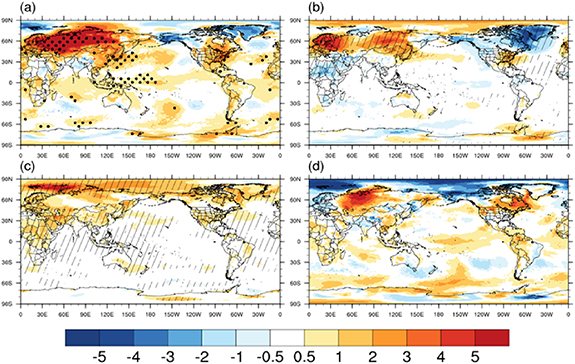
Figure 4. (a) Anomaly of T2m in 2020 with respect to 1979–2019 climatology; black dots mark grid-points where T2m is the highest on record. (b) The AO contribution; thin nets mark the grid-points where the regression coefficient is significant at the 95% confidence level in two-tailed test. (c) The LWT contribution; thin nets mark the grid-points where the linear trend is significant at the 95% confidence level in two-tailed test. (d) The residual of the T2m anomaly in 2020 excluding the AO and LWT contributions (Unit: K).
Download figure:
Standard image High-resolution image3.2. Regional/subregional portion of the JFM 2020 anomalies congruent with the AO and global warming
Table 1 shows the portion of the JFM 2020 observed anomalies congruent with the AO and global warming. For whole East Asia, the average AO contribution accounts for 58% of T2m anomalies, while the LTTs contribute 32%, together they explain 90% of the observed anomalies. Over NEA, the AO portion increases up to 78%, while the global warming contribution accounts for 32%. Summation of these two contributions leads to 10% overestimation of the observed anomalies and essential negative residuals. EEA demonstrates results closest to the observations, 94% of the observed anomalies are congruent with the joint AO and global warming contribution, with the AO accounting for 66% and LTTs for 28%. The poorest results are for SEA, 45% of jointly explained portion of the observed anomaly, with the AO portion being 3% and the global warming portion being 42%. In general, our statistical model, implying contributions by only the AO and global warming, is appropriate for East Asia on regional scale and on the subregional scale for NEA and EEA, for which residuals are about 10% of the observed anomaly. For SEA, where the AO influence is uncertain (figure 3), the only LTTs underestimate anomalies and remain large residual discussed in section 4.2. Results for T2max and T2min resemble those for T2m and are shown in supplementary material (table S1).
Table 1. Regional/subregional JFM 2020 mean observed T2m anomalies and their portions contributed by the AO, LTT, AO + LTT. The positive (negative) residuals correspond to underestimation (overestimation) of the observed anomalies.
| Region/subregion | Mean anomaly (K) | Portion of observed anomaly (%) contributed by | Residual (%) | ||
|---|---|---|---|---|---|
| AO | LTT | AO + LTT | |||
| EA | 2.35 | 58 | 32 | 90 | 10 |
| NEA | 3.02 | 78 | 32 | 110 | −10 |
| EEA | 2.17 | 66 | 28 | 94 | 6 |
| SEA | 1.97 | 3 | 42 | 45 | 55 |
3.3. Particular temperature anomalies and contributions over East Asia
The positive T2m anomalies exceeding 2 K over the land and 1 K over the seas span almost whole East Asia (figure 5(a)), with new records being established in the northernmost NEA (anomalies exceed 5 K in the Lena-Aldan interfluve), most of EEA (anomalies of up to 4 K), and coastal areas of SEA, (anomalies of up to 3 K). The AO contributes positively (1 to 5 K) over NEA and EEA (figure 5(b)). However, the AO positive contribution over SEA is negligible and even locally negative as a result of the low coefficient of determination (<0.1) between observed and estimated T2m (figure 2(b)). The LTTs contribute positively over whole East Asia, with contribution of 1 to 2 K spanning SEA and parts of NEA and EEA (figure 5(c)). Regionally, the AO contribution is the strongest over NEA and weakest over the SEA, while LTTs' is relatively strong over SEA.
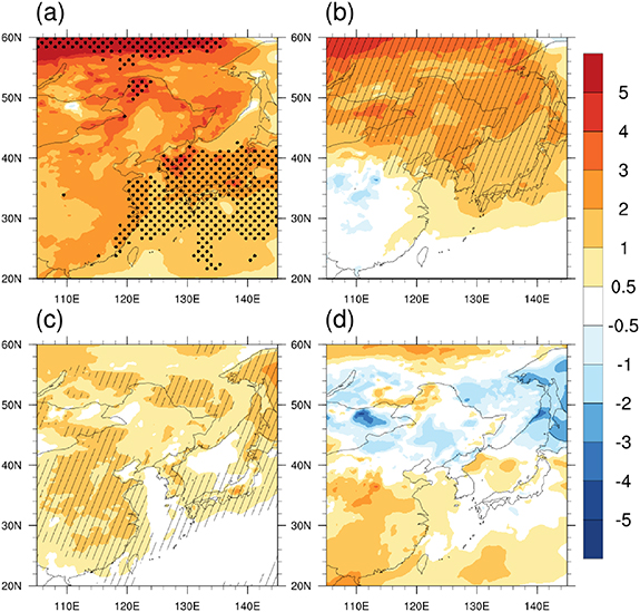
Figure 5. Same as figure 4, but for East Asia.
Download figure:
Standard image High-resolution imageAs shown in figure 5(d), the statistical model underestimates observed anomalies over SEA (residuals of up to 2 K) and over the Lena-Aldan interfluve and Manchuria in NEA (residuals of up to 3 and 2 K). Meanwhile, in the rest of NEA, residuals, mainly negative, are quite small and randomly dispersed over land while the main area of the negative residuals (overestimation) is over the adjacent seas. Over EEA, residuals do not exceed 1 K, with residuals less than 0.5 K spanning the Korean Peninsula and Japanese Archipelago where the observed anomaly extremes achieve 4 K being the highest on record. The detail discussion on the residuals is posted in the section 4.2. For T2min and T2max, the results are similar to those of T2m. Please refer to the supplementary material for details (figures S3 and S4).
3.4. Consistency between the observed and estimated temperature fields
Spatial correlation between the observed T2m field and the field estimated using the LTT is 0.38 while that estimated using AOI is 0.72, that indicates that the AO contribution pattern is closer to the observed anomaly pattern than the LTT contribution.
The RMSE for the T2m field estimated using the LTT (1.95 K) is larger than that associated with the AO (1.34 K) that supports the result from the consistency assessment on the superiority of the AO contribution. Superiority of the AO contribution also results from the significant positive MSSS value (0.53) assessing consistency between the observed field and the AO contribution in respect to the LTT contribution. However, the lowest RMSE (1.00 K) is between the observed field and the field combining both the AO and LTT contributions, meanwhile, the significant positive MSSS value (0.45) proves that it is global warming that essentially improves the field estimated based on the AO alone. The field consistency scores for T2min and T2max are similar to those obtained for T2m, see tables S2 and S3 in supplementary material for detailed values. Consequently, the observed strong positive temperature anomalies including extreme anomalies over East Asia could have been achieved only as a combined effect of the extreme positive AO event and global warming.
4. Discussion
4.1. Relationships between the AO and global warming
Our study is based on assumption of statistical independence between AOI and global warming trend over the 41 year training period during which the AOI trend was negligible. Meanwhile, statistical independence during a certain period does not imply physical independence between the AO and global warming. Particularly, at least two physically plausible mechanisms linking the AO and global warming that offset each other have been suggested. The first mechanism has been detailed and supported in the model studies by Shindell et al (2001). Increase of well mixed greenhouse gas concentration in atmosphere results in increase in horizontal temperature gradient between the upper tropical troposphere and lower polar stratosphere that results in enhancement of the polar vortex, that is, the positive AOI polarity. The second suggested mechanism is based on the Arctic amplification, the enhanced Arctic warming as compared with the middle and lower latitudes caused by the positive feedback between the sea ice retreat and global warming. It must result in decrease of the temperature gradient between middle and polar latitudes, enhancement of meridional circulation and weakening of zonal one, that is, in the negative AOI polarity (Cohen et al 2020, and references therein). However, it should be noted that there is no consensus on the second mechanism yet, with model studies disagreeing each other and observed periods being too short for reliable statistical confirmation (Cohen et al 2020). The first mechanism prevailed in the 1960s–1990s, with the AOI trend during 1959–1997 being 0.041 ± 0.032σ/year. Associated significant contribution to the global warming signals during the 1960s–1990s was demonstrated by Thompson et al (2000) and numerous following studies. However, since the 1990s, the AOI trend has been decreasing down to the negative values (Kryzhov and Gorelits 2015), and the AO signal became distinguishable from that of global warming (Cohen and Barlow 2005). This AOI decrease was possibly caused by the second mechanism.
Our training period comprises both the AOI positive and negative trend periods, with the AOI trend for the whole 41 year training period turning out negligible. We should note that external forcings not related to global warming that may also affect the AO have been also suggested, particularly, variations in ultra-violet solar radiation and volcano eruptions (e.g. Shindell et al 2001). Therefore, if the AOI trend were significant, uncertain would be the causes of the trend, and the AO signal would become undistinguishable from that of global warming in an empirical study. Meanwhile, for the period 1979–2019 when the AO trend is negligible, the AO and global warming signals become distinguishable, so do their contributions to the anomalies of JFM 2020.
We have also analyzed status of the SCE of JFM 2020 which may influence on the AO and East Asia temperature at the same time. As has been shown by Juzbašić et al (2021) development of the extreme positive JFM AO event was abnormal in the autumn and winter of 2019/20. It was preceded by enlarged October and November SCE in Eastern Eurasia that tends to result in the negative AO phase rather than positive (Cohen et al 2007, Cohen and Jones 2011, Han and Sun 2018). However, in spite of the extreme positive JFM AO event, because of its abnormal development, the autumn 2019 area averaged SCE anomaly standardized in respect to 1979–2019 was 0.95 in East Asia. The positive SCE anomaly persisted into winter being 0.56 in JFM 2020, weakening the AO-induced warming impact. Meanwhile, the East Asia JFM SCE negatively correlates with the AO with coefficient −0.44 on the detrended 41 year series.
It is also worth noting that the positive SST anomalies in the equatorial Pacific, with the JFM 2020 Nino3.4 index being 0.5, similarly to the autumn positive SCE anomalies in Eastern Eurasia, were favorable for the negative phase of the AO (Fletcher and Cassou 2015) rather than the extreme positive AO event.
4.2. Residuals
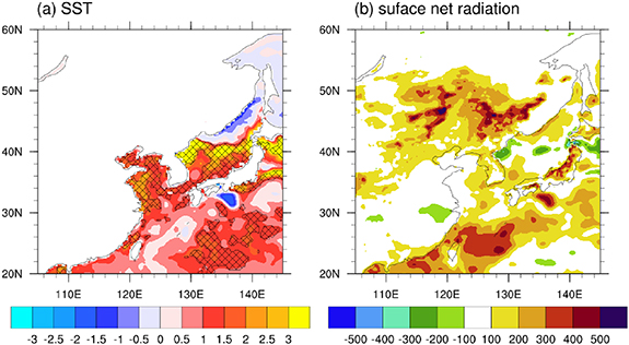
Temperature anomalies are overestimated (negative residuals) by 10% as average over NEA, with the largest negative residuals spanning the seas as a result of underestimation of enhanced cold advection from the continent with anomalous westerlies and prevailing negative SST anomalies (figures 6(a) and S5). The negative residuals in the continental area may be a result from the positive SCE anomaly in NEA, with standardized in respect to 1979–2019 area average SCE anomaly in JFM 2020 being 0.75. On the background of average overestimation, there are two areas of essential underestimation of the observed anomalies those are the northernmost NEA part and the central NEA part over Manchuria. The northernmost area of NEA in JFM 2020 was affected by anomalous westerlies in the western part and southerlies in the eastern part (figure S5), which caused additional heat advection from warmer western domain and from the East Sea (figures 4(d) and 6(a)), not inherent in the classical AO pattern, and could result in the underestimation of anomalies by the model. It should be noted that SST of the East Asia adjacent seas was extremely high in JFM 2020 (figure 6(a)) in contrast to the negative SST anomaly in 1989 when the previous extreme AO event occurred (Juzbašić et al 2021). The area of the positive residuals in Manchuria is a comparatively flat valley bordered in the north with an arc of the trans-Baikal ridges opened to anomalous south-easterlies of JFM 2020 (figure S6). Also, these positive residuals could result from an anomalous radiative forcing during JFM 2020 (figure 6(b)) that corresponds to the enhanced role of radiative forcing in temperature variability in the dryland belt (Groisman et al 2018).
Figure 6. Anomalies of (a) SST (Unit: K) and (b) surface net radiation (Unit: W m−2) in JFM 2020 with respect to 1979–2019 climatology. Thin nets in (a) mark grid-points where SST is the highest on record. The value in (b) was calculated as an algebraic sum of mean surface net shortwave and longwave radiation flux, the positive indicates downwards.
Download figure:
Standard image High-resolution image
Underestimation by 40%–69% of the observed anomalies over SEA, at least in its eastern part where anomalies were extreme, was caused by the anomalous heat advection to the region from the adjacent seas with extremely high SST (figures 6(a) and S5). Given that the tendency of a weaker winter monsoon marked by warmer winters to occur in El Niño years (Ha et al 2012), the extremely high SST could be related to a weak El Niño during JFM 2020. However, both low intensity of El Niño (Nino3.4 index was 0.5) and rather low mosaic distributed correlation between SST in the adjacent seas and the Nino3.4 index, slightly exceeding the 95% confidence level (figure S7), do not imply a strong El Niño impact on East Asia T2m in JFM 2020. Meanwhile, in the north-western continental part anomalous radiative forcing (figure 6(b)) could explain essential underestimation of the observed anomalies by the LTT alone with no additional contribution by the AO.
Analysis of residuals, that is, the portion of the observed anomalies not dominated by global warming and the AO, with both impacts being parameterized on the 1979–2019 series, reveals that the residuals were mainly caused by extremely high SST of the seas adjacent to East Asia, anomalous south-easterlies, and locally anomalous radiative forcing.
5. Conclusion
In recent decades, the occurrences of abnormally high temperatures have increased in frequency and intensity. Global warming caused by Earth's radiative imbalance clearly contributes to this, but its local manifestations are not uniform. It raises the question of whether each new regional temperature extreme is a result from global warming or regional peculiarities, particularly anomalous heat advection with circulation anomalies. The extremely warm winter of 2019/20 gave us a unique opportunity to compare the roles of global warming and the AO in achieving these extremes based on observations.
We performed this analysis for East Asia based on linear LTTs and cubic temperature-AO relationships. The extremely positive AO event accounts for 78% and 66% of the temperature extremes in NEA and EEA, correspondingly, and had a negligible effect for SEA. Moreover, the LTTs made the anomaly patterns estimated by the AO contributions more consistent with those observed in all regions. Notably, the LTTs account for 42% of the anomalies observed in SEA. Meanwhile, the statistical model in this study showed residuals in some regions of NEA and SEA, which appear to be related to the unique climate features of JFM 2020, such as anomalously high SLP over the Northern Pacific and associated anomalous heat advection to East Asia, extremely warm SST along the East Asia coast, and enhanced radiative forcing over Manchuria.
This study suggests that the 2020 wintertime temperature extremes would probably not have occurred in the absence of either the extreme AO event or background global warming and shows that superimposing of certain climate modes on global warming could lead to previously unexperienced extremes in future. These results have implications for the evaluation of possible temperature anomalies caused by the extreme AO events behind steady climate system changes, particularly the temperature's upward trend which matches the goals of NEFI (Groisman et al 2017, Soja and Groisman 2018). It also suggests that appropriate climate change adaptation and mitigation should be implemented as soon as possible in East Asia, as the occurrence of extreme events in response to climate change might pose challenges to sustainable societies.
Acknowledgments
This work was funded by the Korea Meteorological Administration Research and Development Program under Grant No. KMI2020-01411.
ERA5, a fifth-generation ECMWF reanalysis data (Hersbach et al 2018, 2019a, 2019b) are provided by the Copernicus Climate Change Service (C3S) and were obtained from Climate Data Store (CDS) homepage at https://cds.climate.copernicus.eu/. Monthly AO indices are taken from the NOAA Climate Prediction Center website (www.cpc.ncep.noaa.gov/). Snow cover data were provided by Rutgers University (https://climate.rutgers.edu/snowcover/index.php)
Data availability statement
The data that support the findings of this study are available upon reasonable request from the authors.