

Abstract
Temperature extremes have increased during the past several decades and are expected to intensify under current rapid global warming over Southeast Asia (SEA). Exposure to rising temperatures in highly vulnerable regions affects populations, ecosystems, and other elements that may suffer potential losses. Here, we evaluate changes in temperature extremes and future population exposure over SEA at global warming levels (GWLs) of 2.0 °C and 3.0 °C using outputs from the Coupled Model Intercomparison Project Phase 6. Results indicate that temperature extreme indices are projected to increase over SEA at both GWLs, with more significant magnitudes at 3.0 °C. However, daily temperature ranges show a decrease. The substantial increase in total SEA population exposure to heat extremes from 730 million person–days at 2.0 °C GWL to 1200 million person–days at 3.0 °C GWL is mostly contributed by the climate change component, accounting for 48%. In addition, if global warming is restricted well below 2.0 °C, the avoided impacts in population exposure are prominent for most regions over SEA with the largest mitigation in the Philippines. Aggregate population exposure to impacts is decreased by approximately 39% at 2.0 °C GWL, while the interaction component effect, which is associated with increased population and climate change, would decrease by 53%. This indicates serious consequences for growing populations concurrent with global warming impacts if the current fossil-fueled development pathway is adhered to. The present study estimates the risks of increased temperature extremes and population exposure in a warmer future, and further emphasizes the necessity and urgency of implementing climate adaptation and mitigation strategies in SEA.
Export citation and abstract BibTeX RIS

Original content from this work may be used under the terms of the Creative Commons Attribution 4.0 license. Any further distribution of this work must maintain attribution to the author(s) and the title of the work, journal citation and DOI.
1. Introduction
How much time do we have left? The global mean surface temperature (GMST) in 2020 was 1.2 ± 0.1 °C above pre-industrial levels, and was among the three warmest years on record (WMO 2021). Limiting global warming to below 2.0 °C, even to the ambitious target of 1.5 °C, has been a keystone commitment of the Paris Agreement (UNFCCC 2015) under the United Nations Framework Convention on Climate Change (UNFCCC). However, there is not much time left, since the current mitigation strategies for anthropogenic greenhouse gases (GHG) cannot support us to achieve a temperature rise below 1.5 °C, and the ambitious target now seems hardly feasible (Rogelj and Knutti 2016, Smith et al 2019, IPCC 2021). Consequently, climate and weather extremes are very likely to continue in the near future (Stott 2016). It is therefore crucial for the scientific community to deeply understand the future changes in climate extremes, and their consequent impacts on the human society and ecosystem.
It has been widely acknowledged that the occurrences of worldwide temperature extremes are associated with the rise in GMST (WMO 2011, IPCC 2018). Examples include the European heatwave in 2003, which was the warmest record-breaking temperature for hundreds of years, causing at least 20 000 heat-related deaths (Stott et al 2004, Hajat et al 2006, Barriopedro et al 2011, Russo et al 2015) and the extremely hot summer in 2010, when Russia suffered a rare heatwave which caused over 50 000 deaths (Dole et al 2011, Hoag 2014, You et al 2017). Increasing temperature extremes concurrent with incidences of heat-related hazards have been the focus of significant societal concerns over the past two decades (Ishigami et al 2008, Anderson and Bell 2009, Stott et al 2010, Åström et al 2013). Looking ahead to the middle of the 21st century, intensified temperature extremes are expected to occur more frequently with longer durations, resulting in the potential hazard of increased heat-related morbidity and mortality, especially in developing countries with aging populations (McMichael et al 2006, Bindoff et al 2013, Rohat et al 2019). For instance, the increase of high temperatures would amplify adverse impacts on human health through deterioration of existing medical conditions and heat stress, such as respiratory, cerebrovascular and cardiovascular disorders (Bobb et al 2014, Gasparrini et al 2015, Carleton and Hsiang 2016). Thus, it is not only essential to provide detailed information on changes of temperature extremes in the future, but also critical for exploring the impacts of temperature extremes on humans.
Southeast Asia (SEA) is characterized by a dense population with distinct terrains, an area that is generally vulnerable to global warming. Climate conditions of the SEA mainland are significantly modulated by the Asian-Australian monsoon regime (Matsumoto 1997, Webster et al 1998, Wang et al 2001, Zhou et al 2011, Ge et al 2021b) and the El Niño/Southern Oscillation (ENSO; Barnett et al 1999, Wang and Chan 2002, McPhaden et al 2006, Ge et al 2017, McGregor and Ebi 2018). In the past few decades, SEA has already experienced intensified extreme events, imposing widespread heat-related risks that have led to considerable social and economic losses (IPCC 2013, 2021, Zhu et al 2020b, Ge et al 2021a). In April 2016, record-breaking droughts that accompanied long durations of temperature extremes resulted in many deaths and massive socioeconomic impacts (Thirumalai et al 2017). These unprecedented heat extremes are likely to intensify under current rapid global warming (Zhu et al 2020a, Dong et al 2021). Additionally, with a population of more than 600 million across SEA, enhanced severe extremes associated with ongoing global warming would expose more people to danger (Liu et al 2017b, Kumar and Mishra 2020). Since the incidences of heat-related mortality, awareness of temperature extremes has become increasingly important for densely populated areas, where estimating projected changes of population exposure to temperature extremes is essential for local governments in implementing adaptations and mitigations. However, the research on investigating the exposure to temperature extremes in response to different global warming levels (GWLs) remains insufficiently represented. In this work, we focus on population exposure changes to heat extremes in a warmer world over the SEA region, and also address the following key issues. (a) How do temperature extremes over SEA change at 2.0 °C and 3.0 °C GWLs? (b) To what extent could the risk of exposure to heat extremes increase if the GMST rises by 2.0 °C or even more? (c) How much of the impact could be avoided if global warming is limited to 2.0 °C?
2. Data and methods
2.1. Datasets and temperature extreme indices
The daily maximum and daily minimum temperatures in this study are derived from 20 Coupled Model Intercomparison Project Phase 6 (CMIP6) ensembles (supplementary table S1 available online at stacks.iop.org/ERL/17/044006/mmedia, Eyring et al 2016). The future changes in temperature extremes are projected under two Shared Socioeconomic Pathway (SSP) scenarios (SSP2-4.5 and SSP5-8.5, O'Neill et al 2016). They represent the medium part and high end of the ranges of future forcing pathways. In order to evaluate the historical runs of CMIP6 during the period of 1985–2014, the observational datasets of SA-OBSv2.0 covering the period of 1981–2017 derived from Southeast Asian Climate Assessment & Dataset (SACA&D) is selected in this study (Van Den Besselaar et al 2017). It has undergone accurate quality control and is currently one of the high–quality available gridded observational dataset for SEA, which has been widely used to evaluate regional and global climate simulations (Van Der Schrier et al 2016, Van Den Besselaar et al 2017, Ge et al 2019a, Dong et al 2021).
The domain of SEA is located from 10° S to 23° N and 95° E to 140° E and divides into five subregions as shown in figure S1: the Indochina Peninsula (ICP; 6° N–23° N, 95° E–110° E), Kalimantan (KAL; 4° S–6° N, 109° E–118° E), Sumatra (SUM; 8° S–6° N, 95° E–108° E), Philippines (PH; 5° N–20° N, 118° E–130° E), and Sulawesi (SUL; 6° S–3° N, 118° E–126° E).
Table 1 shows the four recommended indices from the Expert Team on Climate Change Detection and Indices (ETCCDI), which are used to estimate the temperature extremes over SEA (You et al 2011, Sillmann et al 2013b, Sheikh et al 2015). Further information could be found at the ETCCDI website, http://etccdi.pacificclimate.org/indices.shtml.
Table 1. Definitions of used temperature extreme indices.
| Label | Index definition | Units |
|---|---|---|
| WSDI | Warm spell duration index (number of days summed by periods where at least six consecutive days when TX > the calendar day 90th percentile centered on a five-day window for the baseline of 1981–2010). | day |
| DTR | Daily temperature range (difference between TX and TN). | °C |
| TX90p | Number of warm days (percentage of days when TX > 90th percentile, where TXij is the daily maximum temperature on day i in period j and TXin90 is the calendar day 90th percentile centered on a five-day window for the baseline of 1981–2010). | % |
| TN90p | Number of warm nights (percentage of days when TN > 90th percentile, where TNij is the daily minimum temperature on day i in period j and TNin90 is the calendar day 90th percentile centered on a five-day window for the baseline of 1981–2010). | % |
Based on assumptions that the population was predominantly influenced by fertility, income, and political change, a new spatial population downscaling model dataset is provided by the National Center for Atmospheric Research and City University of New York Institute for Demographic Research (NCAR-CIDR). Taking into account the uneven economic development of different regions in SEA, we used population projections under SSP3, which is the pathway that faces great challenges of climate change adaptation and mitigation (Jones and O'Neill 2016). Additionally, an event is here defined as a heat extreme when the daily maximum temperature exceeded the threshold corresponding to the 90th percentile of the baseline, in accordance with the TX90p index recommended by the ETCCDI (Batibeniz et al 2020, Iyakaremye et al 2021).
2.2. Definition of GWLs of 2.0 °C and 3.0 °C
The 'time sampling' approach was employed to define the GWLs, since this could eliminate interannual variability and reduce uncertainties from the different models (Vautard et al 2014, King et al 2017, Ge et al 2019b). The pre–industrial reference period is defined as years of 1881–1910, which is available from all CMIP6 historical simulations. In order to get stable climatology states, the 30 year averaged window of the running mean which reached 2.0 °C and 3.0 °C higher than the pre–industrial baseline is identified as the corresponding GWL. According to this approach, seven models under SSP2-4.5 and SSP5-8.5 scenarios reached the 2.0 °C and 3.0 °C thresholds, which together comprise 14 ensemble members for each GWL. The spread of the years covered by the participating outputs is shown in figure 1.
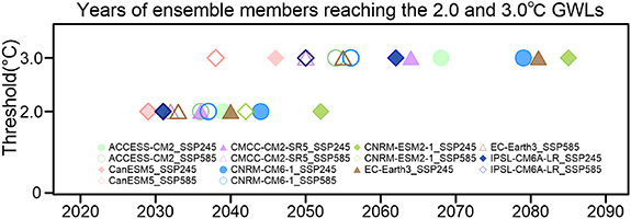
Figure 1. Timing of participating ensemble members reaching 2.0 °C and 3.0 °C GWLs above the 1881–1910 pre-industrial baseline. The years represent the mid-year of 30-year running mean periods.
Download figure:
Standard image High-resolution image2.3. Evaluation of CMIP6 model performances
Here, the relative root mean squared error (RMSE') is applied to evaluate the empirical reliability and the robustness of the model performance (Sillmann et al 2013a, Zhou et al 2014, Zhu et al 2020a)
where  is the ensemble median of RMSEs for all selected models. In general, a better (worse) performance than the majority of the model was represented as negative (positive) RMSE'.
To assess the interannual variability of the models relative to the observations, the interannual variability skill score (IVS, Gleckler et al 2008, Yang et al 2021) is used and calculated as
where SDm and SDo are the standard deviations of the model simulations and observations, respectively. IVS is a symmetric variability statistic to quantitatively estimate the interannual variation, with smaller value indicates better agreement with the observational data. The CMIP6 model outputs are interpolated onto a common horizontal resolution of 1° × 1° by bilinear interpolation to keep consistency with the SA-OBSv2.0 observations.
Figure 2 presents the statistical metrics of the temperature extreme simulations in selected models relative to the SA-OBSv2.0 observations. It can be seen that the models vary considerably in simulating temperature extremes. Most of the models show relatively better modeling performance, especially EC-Earth3 and IPSL-CM6A-LR. Their correlations range among 0.5–0.9 and the ratios of standard deviations (RSD) are generally close to 1 (see text S1 in the supplementary material for equations). However, relatively 'weak' performance occurs in simulation from CMCC-CM2-SR5, with positive RMSE' values for all indices except TX90p. Overall, lighter colors represent a better model performance. The ensemble medians with lighter colors are superior to each single model in each respect, the IVS values are below 1.5 for all indices (figure 2, last row). This suggests that the ensemble median can reasonably represent the results of the future projections, which reduce the uncertainties of the participating models to a great extent and is therefore determined to represent the projected changes in the following study.
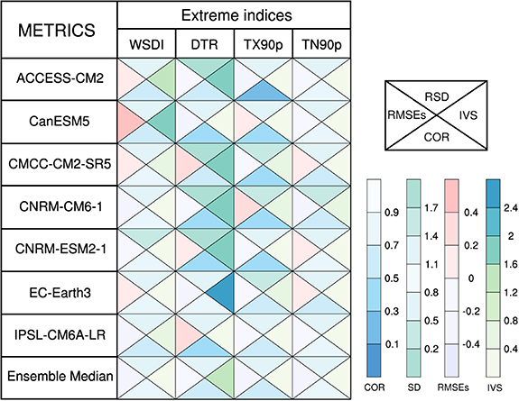
Figure 2. Statistical metrics in temperature extreme indices based on the participating CMIP6 ensemble members versus the SA-OBS observations during the period of 1985–2014. COR is the correlation coefficient, RSD is the ratio of standard deviation, RMSE' is relative root mean squared error and IVS is interannual variability skill score.
Download figure:
Standard image High-resolution image2.4. Quantitative estimations of population exposure and avoided impacts
Population exposure to heat extremes is calculated by multiplying the projected frequency of warm days (TX90p) in each grid point and the projected population for each corresponding point (Liu et al 2017b, Chen and Sun 2019). Here, we estimate the population exposure change following the approach of Jones et al (2015), and typically decomposed into three terms (equation (3))

where ΔE is the total population exposure changes, C1 and P1 are the heat extremes and population of the baseline, respectively. ΔC and ΔP are the changes in heat extremes and the population in the warmer world relative to the base time. Hence, P1 × ΔC, C1 × ΔP and ΔC × ΔP represent the climate effect, population effect and their interaction effect on exposure change.
Finally, the avoided impacts (AI) of exposure change due to the lower warming are calculated as follows:
where C2.0 and C3.0 are the changes of heat extremes (represented by TX90p) and population exposure under the 2.0 °C and 3.0 °C warmer climates, respectively. Here, the two-tailed Student's t-test is employed to verify all statistical significances at the 95% confidence level.
3. Results
3.1. Future projections in temperature extremes at 2.0 °C and 3.0 °C GWLs
Future changes in temperature extremes over SEA at 2.0 °C and 3.0 °C GWLs are presented in figure 3, respectively. Temperature extremes are projected to show a general increase over SEA at different GWLs, except for daily temperature range (DTR). These projected changes are substantially greater in some regions over SEA, with disproportionate spatial magnitudes and extents. It is noteworthy that more significant temperature extremes can be found at the 3.0 °C GWL than at the 2.0 °C GWL. The three indices of warm spell duration index (WSDI), TX90p and TN90p (representing the warm spell duration index, number of warm days and number of warm nights, respectively; see table 1) are projected to intensify significantly over Maritime Continent at both GWLs. They also share similar spatial distributions, which show that the increases over the Indochina Peninsula (ICP) are smaller than those over the Maritime Continent. Future changes in WSDI at both GWLs indicate longer warm spell duration would be existed over SEA. Over the Maritime Continent, a prominent amplification of WSDI by 43 days would exist at the 2.0 °C GWL, which would further increase by 18 days and especially even reach 90 days in some areas at the 3.0 °C GWL. For TX90p, the largest increase occurs across the PH, and with an increase of approximately 40 days in response to a warmer future. Higher TX90p and TN90p imply that intensified temperature extremes would occur more frequently and also that the change in nighttime warming will slightly exceed that of daytime. The increases in warm nights could be attributed to the high temperature and wet climate at nighttime, which tend to pose more heat stress (Li et al 2018, Liao et al 2018, Ullah et al 2019). An increasing probability of adverse impacts exert on public health, especially for those countries with dense coastal population. These indices of relative thresholds can capture warm weather under various climatological conditions (Radinović and Ćurić 2012, Sillmann et al 2013b).
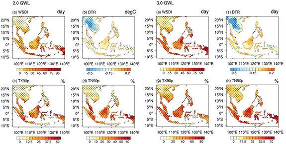
Figure 3. The future changes of CMIP6 ensemble median in temperature extreme indices at the 2.0 °C and 3.0 °C GWLs relative to 1985–2014. The black dots represent ensemble medians are significant at the 95% confidence level.
Download figure:
Standard image High-resolution imageOn the other hand, the projections show anomalous decreases of DTR that occur in the central areas of the ICP at both GWLs, which could be mainly attributed to inconsistent rapid increases in maximum and minimum temperatures (Horton 1995, Caesar et al 2006, Martínez et al 2010, Yao et al 2013). This also suggests that the decreased DTR are closely associated with the increasing number of warm days (TX90p) and warm nights (TN90p), confirming a potential risk of aggravated heat extremes under the acceleration of global warming. This result is also consistent with our conclusions from CORDEX model ensembles (Zhu et al 2020a).
3.2. Future population exposure at 2.0 °C and 3.0 °C GWLs
Changes in temperature extremes and population combine to drive exposure. In this section, we estimate the future changes in population exposure over SEA and the subregions at two GWLs, as shown in figure 4. Generally, changes in projected exposure show a distinctly great increase in different GWLs. Notably, the ensemble medians of the total projected exposure changes (ΔE) exhibit a particularly large increase at the 3.0 °C GWL, suggesting a higher population exposure will be established at future warmer world. For the SEA region as a whole (figure 4(f)), the median of the total exposure to heat extremes (TX90p) increases by 205% under the 2.0 °C GWL while that value rises to 337% under the 3.0 °C GWL. For the subregions, striking increases in exposure are projected with magnitudes of 549% and 1094% over the PH at the 2.0 °C and 3.0 °C GWLs, respectively. Over KAL, projected exposure changes increase by 316% (513%) at the 2.0 °C GWL (3.0 °C GWL). The total exposure changes become moderate in the ICP compared with other regions. If temperatures reach 3.0 °C of warming, the ICP has an increase of 202% in exposure changes. Although the increasing magnitude is smaller than in other regions, the absolute change under the two GWLs is still dramatic, which emphasizes the necessity of limiting global warming. In general, these results imply that the risks of population exposure would be further exacerbated over the entire SEA under the higher warming scenarios.
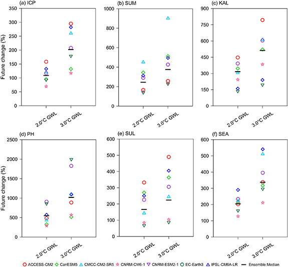
Figure 4. Total population exposure change (ΔE) to heat extremes (TX90p) during 2.0 °C and 3.0 °C warming periods compared with the base time during 1985–2014 in SEA and subregions (unit: %).
Download figure:
Standard image High-resolution imageTo quantify the relative importance of the different drivers to population exposure, we further used equation (3) to estimate the total exposure change and its components (including the climate change component, P1 × ΔC, the population change component, C1 × ΔP, and the interaction component, ΔC × ΔP) for different regions at 2.0 °C and 3.0 °C GWLs (figure 5). Under the 3.0 °C GWL, the tendency of exposure change is drastically increased compared with the 2.0 °C GWL, reaching more than 1200 million person-days over SEA, equivalent to a threefold increase relative to the reference period of 1985–2014. Overall, the increase in population exposure over SEA is largely attributed to the climate change component, which accounting for 590 million person-days, while the population and their interaction effects contributed to an increase of 177 million person-days and 434 million person-days, respectively.
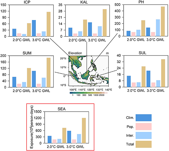
Figure 5. Decomposition of future changes in population exposure at the 2.0 °C and 3.0 °C GWLs over SEA and subregions. Average increase in total population exposure change (ΔE) is shown in brown; exposure change contributed by climate effect in dark blue; exposure change contributed by population effect in pink; and exposure change contributed by interaction effect in light blue (see section 2 for details) (units: person-day, 106).
Download figure:
Standard image High-resolution imageAt the regional scale, the climate change component also has more far–reaching influence on the increase in exposure change, as substantially greater exposure always contributes by climate change than population change, particular in the ICP and SUM. For example, the increased exposure in SUM is primarily from the contribution of climate effect, which accounts for 66 million person-days, followed by the attributable portion from interaction effects for 33 million person-days. The population effect can be observed a relatively small proportion in increased exposure at a warmer climate, accounting for approximately 22 million person-days. In other words, 54% of the increase is induced by the climate change component.
In contrast, the intensified heat extremes over the KAL have relatively moderate impact on local exposure as a result of the low population density. The exposure increases by 30 million person-days in the future (at 3.0 °C GWL), exceeding fivefold with respect to the current climate. However, greater impacts occur over PH from the interaction component than other two components. The increase in exposure goes from around 253 million person-days at 2.0 °C GWL to 470 million person-days at 3.0 °C GWL. This is largely due to the widespread increase in heat extremes coinciding with higher population density. Under such warming, an increase caused by the interaction component strengthens over the PH, to 102 million person-days and 267 million person-days, respectively, under the two scenarios.
In brief, for both SEA as a whole and the subregions, increased population exposure is to a great extent associated with climate change in the future. Therefore, the explicit target of restricting climate warming is undoubtedly more beneficial than other climate events and avoided impacts and climate actions should be encouraged to promote such restricting regardless of the mitigation and adaptation strategies in this region.
3.3. Avoided impacts due to limiting warming
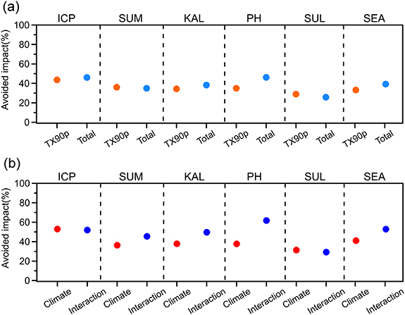
The future projection of the CMIP6 ensembles in climate simulating indicate that the occurrences of heat extremes are expected to intensify at a rate that is unprecedented in the majority regions over SEA as global warming continuous (Kim et al 2020, Chen et al 2020b). If the Paris Agreement goal of limiting the rise below 2.0 °C is met, some temperature extreme events will not be tested. We therefore estimate the avoided impacts of heat extremes and population exposure in response to 1.0 °C limited warming (figure 6). Our results show that nearly all regions would see considerable avoided impacts, although the magnitudes differ among regions. For the whole of SEA, the increase of heat extremes (TX90p, figure 6(a)) can be avoided by approximately 33% in the situation of the 1.0 °C limiting warming, and the increase of population exposure is also avoided by 39% when compared with that under the 3.0 °C GWL. It is notable that the most pronounced changes can be found in the regions of the ICP and PH, where limited 1.0 °C warming will help to avoid increase in heat extremes by at least 40%, and the increase of population exposure can be avoided by 50% in the future. The change tendencies of heat extremes and population exposure are consistent, which also illustrates that climate change is the essential role in driving the increased population exposure. Over the regions of SUL, population exposure presents a moderate reduction in response to the 1.0 °C limited warming, of approximately 29%. Generally, population exposure would be drastically lowered across SEA when GMST increase is controlled below 2.0 °C.
Figure 6. Avoided impact (AI, unit: %) of (a) heat extremes (TX90p) and total population exposure change (ΔE), and (b) climate (P1 × ΔC) and interaction (ΔC × ΔP) components in SEA and subregions.
Download figure:
Standard image High-resolution image
Surprisingly, regarding the decomposed components of exposure, the avoided impacts of population exposure caused by the interaction component over SEA are higher than for the single climate effect (figure 6(b)). The increase of exposure in PH caused by the interaction component (ΔC × ΔP) would be significantly decreased by 62%, while only 38% by the climate component (P1 × ΔC). Over SEA, the interaction component avoids the impacts by more than 50%. These results indicate that the combined effects of increased population concurrent with climate change would induce more risks of population exposure in a warmer future. More efforts to control rapid global warming and increasing populations would lead to more impacts being avoided in the future.
4. Conclusions and discussion
Heat extremes have imposed huge social and ecological stresses in the last few decades. If global warming continues, heat extremes are expected to be more frequent and will exert a negative impact on humans and ecosystems. It is critical for researchers to quantify the potential risk of heat extremes to populations. In this study, we have evaluated the responses of heat extremes at different GWLs against the present day (1985–2014) and the corresponding impacts on population exposure over SEA. The major results are listed below:
- (a)Projected changes of indices indicate distinct increases at 2.0 °C and 3.0 °C GWLs over SEA, with the exception of decreasing DTR. Additionally, future changes in most indices are prominent under the 3.0 GWL compared with the 2.0 °C lower GWL. The regional scale projections of temperature extremes show disproportionate spatial magnitudes and extents. The most significant changes are found in WSDI and TX90p. The increases of TX90p are projected in the PH with the magnitudes of 18% and 47% at the 2.0 °C and 3.0 °C GWLs, respectively.
- (b)Population exposure is projected to increase substantially across the continent in a warmer future. For the SEA region as a whole, the median of the total exposure change to heat extremes would increase by 205% under 2.0 °C GWL, rising to 337% under 3.0 °C GWL. There are significant variations in total exposure over each region, and the PH is expected to experience the largest proportion of increase compared to the present day. The amount of people hit by heat extremes will increase drastically, and the climate effect is a stronger determinant of increased exposure in most regions of SEA.
- (c)Aggregate population exposure over SEA would avoid impacts by 39% if the GMST increase is stabilized at 2.0 °C rather than 3.0 °C, when the interaction component effect (ΔC × ΔP) would decrease by 53% and the climate component effect (P1 × ΔC) by 41%. Meanwhile, the limited warming under 2.0 °C GWL would help avoid heat extremes of 33%. It is notable that the most pronounced changes can be found in the PH regions, where the interaction component effect could decrease approximately 62% in response to the limited warming, suggesting the high risks of increased populations concurrent with climate warming.
SEA, located in the tropics, comprises many developing countries. Low adaptability and rapid population growth make these areas particularly vulnerable to climate change. Our results highlight the concerning rate of heat extremes increases in recent decades. If no action is taken to reduce GHG emissions and other factors contributing to global warming, rising temperature would pose more profound threats to humans (IPCC 2014, Mora et al 2017, Harrington and Otto 2018). In general, climate and population effects are both crucial factors for the increase in population exposure over most regions across the world (Chen et al 2020a). Jones et al (2018) considered that the low contribution of the population effect may be from the urban heat effect resulting in an increasing number of heat extreme days, and that different assumptions concerning internal migration may lead to an increased population in colder areas, accordingly weakening the perceived importance of demographic change. The rise in global temperature plays an increasingly important role in the changes of population exposure. By the mid-21st century, the US population is projected to increase by 50% with reference to the 2005 levels, which would result in more than 161 million people (close to half of the current US population) being exposed to climate extremes per year (Batibeniz et al 2020). In general, these extreme changes of climate characteristics in the coming future are more likely to bring unprecedented pressure to social and ecological environments.
Additionally, the most destructive heat extremes in history were usually manifested in compound heatwaves during daytime and nighttime (Kunkel et al 1996, Meehl and Tebaldi 2004, Mukherjee and Mishra 2018). In fact, daytime and nighttime heat extremes are not completely separated and compound extremes have appeared more frequently in the recent past, such that compound heatwaves have become the most prominent type of heatwave in recent years (Zscheischler et al 2018, An and Zuo 2021). By the end of the 21st century, the rising GHG emissions would make three-quarters of a typical summer experience compound heat extremes, which would induce increased population exposure several times (Wang et al 2020). As well as this, urbanization further enhances societal vulnerability to exert a significant effect, which may even result in more frequent compound heat extremes (Xie et al 2020, Wang et al 2021). More work associated with compound temperature extremes based on CMIP6 model simulations over SEA is therefore urgently needed in the future, and should be combined with the discussion on mitigation targets and liability considerations.
It should be noted that the threshold estimation might be limited due to the relatively small subset of model simulations from CMIP6 up to the launch of the study. The preliminary result provides fundamental understandings on the response to different global warming thresholds over SEA, which are expected to be further examined as more models are added. Besides, it is also indicated that the CanESM5 model is characterized by generally higher climate sensitivities and manifests an earlier emergence of the global warming thresholds than other models. Although its warming projection results have been included in this study, more detailed and comprehensive clarification is necessary for further investigation and discussion (Swart et al 2019, Cook et al 2020, Li et al 2021, Xu et al 2021). Looking ahead, to better evaluate the regional changes in response to different GWLs, higher resolution convection-permitting models with physical parameterizations should be adopted in the subsequent research, which could provide further reliable climate projections over SEA (Prein et al 2015, Liu et al 2017a, Zhao et al 2021).
Acknowledgments
We thank the German Climate Computing Center (DKRZ), ETCCDI, SACA&D, and the climate modeling groups (shown in table S1) for their data and resources. We also acknowledge the support of Chengdu Plain Urban Meteorology and Environment Observation and Research Station of Sichuan Province.
Data availability statement
CMIP6 outputs can be obtained from https://esgf-data.dkrz.de/search/cmip6-dkrz/. The observation datasets are available at https://sacad.database.bmkg.go.id/. Spatial population dataset is provided by www.cgd.ucar.edu/iam/modeling/spatial-population-scenarios.html.
Funding
The National Natural Science Foundation of China (U20A2097, 4210050408).