

Abstract
Australian heatwaves have a significant impact on society. Most previous studies focus on understanding them in terms of frequency, duration, intensity, and timing. However, understanding the spatial characteristics of heatwaves, particularly those occurring in contiguous regions at the same time (here referred to as contiguous heatwaves), is still largely unexplored. Here, we analyse changes in spatial characteristics of contiguous heatwaves in Australia during 1958–2020 using observational data. Our results show that extremely large contiguous heatwaves are covering significantly larger areas and getting significantly longer during the recent period (1989/90–2019/20) compared to the historical period (1958/59–1988/89). We also investigated the association of contiguous heatwaves in Australia with interactions of the El Niño–Southern Oscillation (ENSO) and Indian Ocean Dipole (IOD) using a large multi-member ensemble of a physical climate model. We found that areal magnitude, total area, median duration, and maximum area of large and extremely large contiguous heatwaves in Australia are significantly higher (lower) during the strong El Niño (Es), strong El Niño co-occurring with strong IOD positive (Es-IPs), and with moderate IOD positive (Es-IPm) (co-occurring strong La Niña with the strong IOD negative (Ls-INs)) seasons relative to the neutral seasons (where both ENSO and IOD are in neutral phase). During the Es, Es-IPm, and Es-IPs seasons, the large-scale physical mechanisms are characterised by anticyclonic highs over the southeast and cyclonic lows over the northwest of Australia, favouring the occurrence and intensification of heatwaves in Australia. These results provide insights into the driving mechanisms of contiguous heatwaves in Australia.
Export citation and abstract BibTeX RIS

Original content from this work may be used under the terms of the Creative Commons Attribution 4.0 license. Any further distribution of this work must maintain attribution to the author(s) and the title of the work, journal citation and DOI.
1. Introduction
Heatwaves are generating extra heat at an increasingly rapid rate in recent decades compared to earlier periods over many parts of the world (Perkins-Kirkpatrick and Lewis 2020), including Australia (Reddy et al 2021a). Moreover, heatwaves are projected to increase in frequency, magnitude, and duration in the future climate under higher emission scenarios (Cowan et al 2014, Perkins-Kirkpatrick et al 2017). Australian heatwaves have significant impacts on human health (Loridan et al 2016), crop productivity (Asseng et al 2011), infrastructure failure (McEvoy et al 2012) and can also influence other extreme events like bushfires (Sharples et al 2016, Reddy et al 2021b). For instance, a severe heatwave prior to the 2009 Black Saturday bushfires in Victoria had killed 374 people (Department of Health & Human Services 2009, ABS 2010) and primed the landscape for devastating bushfires (Sullivan and Matthews 2013), which killed an additional 173 people (Teague et al 2010).
In general, heatwaves are defined as episodes of successive days with temperatures exceeding extreme thresholds. Many previous studies have measured heatwaves tracking temporally at a point or grid cell level by employing metrics such as frequency, duration, and magnitude (Fischer and Schär 2010, Perkins and Alexander 2013, Russo et al 2014). Some earlier studies measured the spatial extent of the heatwaves by considering the proportion of grid cells where heatwaves occurred (Russo et al 2015, Sharma and Mujumdar 2017). However, these previous studies did not consider spatial connectivity and did not examine changes in spatial extent of heatwaves occurring over contiguous regions (contiguous heatwaves, hereafter). The spatial extent covered by contiguous heatwaves varies through time (Vogel et al 2020). Hence, tracking heatwaves simultaneously both in space and time dimensions (i.e. three-dimensional) by considering their spatiotemporal connectivity allows us to effectively analyse the areal extent of contiguous heatwaves (Lyon et al 2019, Vogel et al 2020).
Only a few previous studies have investigated the spatial extent of contiguous heatwaves. Lyon et al (2019) analysed these events across the United States and noticed increasing spatial extent under the RCP8.5 emission scenario. Keellings and Moradkhani (2020) examined the spatiotemporal evolution of contiguous heatwaves over different climate regions of the United States in the historical period (1981–2018), observing a substantial increase in the spatial coverage of contiguous heatwaves. Vogel et al (2020) investigated projections of large contiguous heatwaves globally by considering neighbouring countries as contiguous regions and found that they will substantially increase under the RCP8.5 emissions scenario. Over Australia, King and Reeder (2021) tracked spatially contiguous extreme heat events (not necessarily heatwaves) in the southeast during 1979–2018 to explore their lifecycle. However, contiguous heatwaves have not yet been a research focus of Australian heatwaves.
Heatwaves across many global regions (Luo and Lau 2019, 2020), including Australia (Pezza et al 2012, Perkins et al 2015), are influenced by natural climate variability modes through the alteration of atmospheric background conditions, favouring the development and amplification of heatwaves. The El Niño Southern Oscillation (ENSO) (Trenberth 1997), the Indian Ocean Dipole (IOD) (Saji et al 1999), and the Southern Annular Mode (SAM) (Trenberth 1980) have been shown to influence Australian heatwaves, but the strength of their influence differs across the country (Perkins et al 2015, Loughran et al 2017). ENSO and IOD have an effect on heatwaves over large parts of Australia, and the SAM influences heatwaves over a smaller portion of southeast Australia (Perkins et al 2015, Loughran et al 2017). Previous studies highlighted that ENSO and IOD interact with each other (Meyers et al 2007, Risbey et al 2009, Ummenhofer et al 2011). However, the influence of these co-occurring modes of variability on contiguous heatwaves in Australia has not yet been researched.
The short availability of reliable observational data provides only a small sample of the occurrences of various co-occurring modes of ENSO and IOD, making it challenging to comprehensively study the interactive influence of ENSO and IOD on contiguous heatwaves. Previous studies suggest that a single model initial-condition large ensemble (SMILE) with enough members enables the robust quantification of the influence of climate variability (Fischer et al 2018, Lehner et al 2020, Maher et al 2020). Earlier studies used the SMILE to quantify the effects of overall climate variability on climate extremes (Perkins-Kirkpatrick et al 2017, Schaller et al 2018, Deng et al 2021). However, investigating the interactive influence of climate variability modes on contiguous heatwaves in Australia using a SMILE has not yet been conducted.
Here, we examine the observed changes in contiguous heatwaves over Australia during 1958–2020 by simultaneous spatiotemporal tracking. This analysis will provide an understanding of how spatiotemporal characteristics of contiguous heatwaves have changed in Australia during the historical period. We also investigate the influence of co-occurring modes of ENSO and IOD on large contiguous heatwaves in Australia. This investigation provides insights into the driving mechanisms of large contiguous heatwaves over Australia, which may aid in improving their seasonal predictability.
2. Methods
2.1. Data
To identify heatwaves, we employ the daily maximum and minimum temperature data from the Australian Water Availability Project (AWAP) observational gridded dataset (Jones et al 2009). The gridded dataset is developed using the hybrid gridding algorithm on high-quality station data across Australia (Jones et al 2009). The AWAP data is available at both 0.05° and 0.25° horizontal resolutions. We use the 0.25° spatial resolution data for the analysis because of computational limitations and also because it has been suggested that this decrease in grid resolution does not affect the spatial pattern and magnitude of heatwaves (Perkins and Alexander 2013). We use the observed Hadley Centre Global Sea Ice and Sea Surface Temperature (HadISST) monthly global sea surface temperature (SST) data (Rayner et al 2003) for the identification of climate variability modes (ENSO and IOD) during 1958–2020.
Due to the small observational sample size, we obtain daily maximum and minimum temperature and monthly SST data from the CNRM-CM6-1 SMILE (Voldoire et al 2019) of CMIP6 for the historical period 1958–2014 (November 1958–March 2014). Out of the 30 ensemble members (r(1–30)i1p1f2) of CNRM-CM6-1 SMILE, r2i1p1f2 and r25i1p1f2 members data is not considered for the analysis due to large errors in the calculation of contiguous heatwaves compared with the observational data (further details provided in supplementary material (available online at stacks.iop.org/ERL/17/014004/mmedia)). These 28 ensemble members of CNRM-CM6-1 SMILE provides a large sample size to robustly investigate the interactive influence of ENSO and IOD on contiguous heatwaves in Australia (Schaller et al 2018, Lehner et al 2020). We choose CNRM-CM6-1 SMILE because it performs well in simulating extreme temperatures across Australia (Deng et al 2021), and its horizontal resolution is finer (1.4008° × 1.40625°) compared to other SMILEs of CMIP6. A finer resolution is required to effectively capture the spatial variation of contiguous heatwaves across various climatic regions and coastlines of Australia, where a relatively coarser resolution would provide fewer grid cells, if any at all (Perkins et al 2014).
2.2. Contiguous heatwaves
We defined heatwaves at each grid cell using the excess heat factor (EHF) (Nairn and Fawcett 2013), which has been used in many previous Australian heatwave studies (Perkins et al 2015, Reddy et al 2021a). The EHF is computed according to Reddy et al (2021a) and is expressed in the supplementary information (equations (S1)–(S4)). The EHF based heatwave definition identifies a heatwave as a period of three or more consecutive days with a positive EHF value (>0). However, recent research shows that heatwaves can continue after minor interruptions of cold days, and these heatwaves could have similar effects to those that persist through consecutive days (Baldwin et al 2019). To overcome this limitation and following Baldwin et al (2019) and Rastogi et al (2020), we allow for minor breaks in our heatwave definition. Therefore, a heatwave at a given grid cell is defined as a period of at least three consecutive days with an EHF value greater than zero, and the heatwave is considered to continue until at least two consecutive days with EHF value less than or equal to zero are recorded.
Contiguous heatwaves are identified using the three-dimensional connected component algorithm (Silversmith 2021). First, the gridded temperature data is converted into binary format, with a '1' assigned to grid cells that satisfy the heatwave criteria described above, and a '0' assigned to those grid cells that do not. Then, the three-dimensional connected component algorithm is applied to the gridded binary data by setting the connectivity as 26, which considers all the surrounding neighbours (9 in the previous day + 8 in current day + 9 in next day) by both adjacent and diagonal connectivity (Vogel et al 2020 see figure 1). This allows tracking the contiguous heatwave simultaneously, both in space and time dimensions. This algorithm also allows a contiguous heatwave event to break into parts and connect again providing they are contiguous either in space or in time. Figure 1 shows the tracking of contiguous heatwaves from 23 January 2009 to 09 February 2009, where each colour represents the different individual contiguous heatwave. The large and long event (represented in red, shown in figure 1) started as a small event on 23 January 2009 and through time grew bigger, moved in space, broke into parts, and connected again and vice versa. During the period 23 January–09 February 2009 several other contiguous heatwaves evolved in space and time, which are shown in different colours (see figure 1).
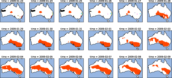
Figure 1. Evolution of contiguous heatwaves over Australian region during the period 23 January 2009–09 February 2009. Each colour represents different individual contiguous heatwave.
Download figure:
Standard image High-resolution image2.3. Contiguous heatwave metrics
Contiguous heatwaves can be quantified by their total area, maximum area, median duration (Vogel et al 2020), and areal magnitude (Keellings and Moradkhani 2020). They are expressed as follows:
- Total area: The sum of the areal extent of a contiguous heatwave across all days.
- Maximum area: The maximum areal coverage of a contiguous heatwave in its duration.
- Median duration: The median value of the duration of all grid cells associated with the contiguous heatwave.
- Areal magnitude: Computed similarly as heat severity and convergence index defined by Keellings and Moradkhani (2020):
where  is the EHF value corresponding to the grid cell
  ,
,  represents the total number of grid cells associated with the heatwave on a particular day
  ,
,  represents the proportion of land area coverage of a heatwave event on a particular day
  ,
,  is the heatwave duration measured in days.
We categorised contiguous heatwaves as large and extremely large events using their total area metric. A heatwave is classified as large or extremely large if its total area exceeds the climatological 80th or 90th percentile value of the selected base period (1961–90), respectively. We focus on analysing the changes in large or extremely large contiguous heatwaves because previous studies have indicated large contiguous heatwaves potentially cause adverse societal impacts such as increased electricity supply-demand, overwhelming pressure on emergency services, and food supply-demand rise in other regions (Lyon et al 2019, Vogel et al 2020), and which will likely have similar impacts for Australia.
The contiguous heatwave metrics of individual events were calculated using the AWAP gridded data across Australia in the extended heatwave season, i.e. from November to March during the period 1958–2020. We used the bootstrapped two-sample Kolmogorov-Smirnov (KS) test (Sekhon 2011) (further details provided in the supplementary material) to identify significant changes or shifts in large and extremely large contiguous heatwave metrics between the first half (1958/59–1988/89) and the second half (1989/90–2019/20) of the study period. We also calculated the seasonal contiguous heatwave metrics of all, large and extremely large heatwaves to see how they are changing through time. The seasonal contiguous heatwave metrics are calculated as follows:
- Accumulated areal magnitude: Seasonal sum of areal magnitude across all contiguous heatwaves (Keellings and Moradkhani 2020).
- Aggregate total area: Comprehensive sum of all individual contiguous heatwave's total area in a season.
- Maximum of maximum area: Maximum value of all individual contiguous heatwave's maximum area in a season.
- Mean of median duration: Average value of all individual contiguous heatwave's median duration in a season.
These seasonal metrics are used to visualise and capture the temporal changes of the respective metric, and in the rest of the study, we considered the individual contiguous heatwave metrics for the analysis.
2.4. Evaluation of CNRM-CM6-1 SMILE
The single realisation or the ensemble mean of the model will not be able to exactly reproduce the observations but can provide the better estimates of temporal variability (Wood et al 2021). Here, to evaluate the model's skill in representing the temporal variability of contiguous heatwaves, we considered the evaluation method followed by the Maher et al (2019), Suarez-Gutierrez et al (2020) and Wood et al (2021). By following this method, we compared the observed seasonal anomalies of contiguous heatwave metrics with the anomalies of the CNRM-CM6-1 SMILE members. Anomalies were calculated relative to the selected base period 1961–90. The model is considered to be overestimating the temporal variability if the observed anomalies cluster mostly (more than 85% of the time) in the 75th percentile range (i.e. 12.5th–87.5th percentile) of the ensemble and many (more than 15%) observations located outside the ensemble range (0–100th percentile) indicates the underestimation of variability. The model is considered to be in a good agreement with the observations in terms of representing the variability when only a few observed anomalies (less than 15%) fall outside the ensemble range and observations should not cluster most of the time (less than 85%) in the 75th percentile range of the ensemble.
2.5. Natural climate variability modes—ENSO and IOD
We used both the HadISST (Rayner et al
2003) and CNRM-CM6-1 SMILE (Voldoire et al
2019) detrended monthly SST data for the calculation of ENSO and IOD indices. The Niño3.4 SST index is used to quantify ENSO (Trenberth 1997). The anomalies were calculated relative to the base period 1961–90. Perkins et al (2015) found that the strength of ENSO is significantly correlated with heatwaves (not necessarily contiguous) over much of Australia. To accommodate the strength variations of ENSO in our analysis, we classified ENSO into two categories (moderate and strong events) according to Casselman et al (2021). Moderate events are defined as ±0.5–1 standard deviation ( ) of mean November–February Niño3.4 index, and strong events are defined as the exceedance of ±1
 of mean November–February Niño3.4 index (see equation (2)):
IOD is quantified using the dipole mode index (DMI) (Saji et al
1999). Similar to ENSO, we classified IOD as moderate and strong events to incorporate the strength variations of IOD in our analysis. Moderate events are defined as ±0.5–1 standard deviation ( ) of mean September–November DMI, and strong events are defined as the exceedance of ±1σ of mean September–November DMI (see equation (3)):
We considered the co-occurring modes of ENSO and IOD to identify their relationship with contiguous heatwaves because these modes can interact with each other (Meyers et al 2007, Risbey et al 2009, Ummenhofer et al 2011). The above-mentioned ENSO and IOD classification resulted in 25 combinations (5 × 5) of phases of co-occurring modes (table 1). For example, the season is considered a strong El Niño active season (Es) only when ENSO is in a strong El Niño phase and IOD in a neutral phase. If ENSO is in a strong El Niño phase and IOD in a strong positive phase, it is considered a co-occurring event strong El Niño + strong IOD positive (Es-Ips). The season is considered neutral (NN) when both the ENSO and IOD are in their neutral phases, respectively. If ENSO is in a strong La Niña phase and IOD in a moderate negative phase, it is considered a co-occurring event strong La Niña + moderate IOD negative (Ls-Inm) (table 1).
Table 1. Description of the total 25 combinations of co-occurring ENSO and IOD phases and presented the frequency of occurrences of these phases in both observational (1958–2020) and CNRM-CM6-1 ensemble data (1958–2014).
| Phase | Number of seasons in the observed HadISST data | Number of seasons in the CNRM-CM6-1 ensemble data |
|---|---|---|
| Moderate El Niño + IOD neutral (Em) | 6 | 83 |
| Strong El Niño + IOD neutral (Es) | 3 | 61 |
| Moderate La Niña + IOD neutral (Lm) | 6 | 50 |
| Strong La Niña + IOD neutral (Ls) | 2 | 64 |
| Moderate IOD positive + ENSO neutral (Ipm) | 2 | 127 |
| Strong IOD positive + ENSO neutral (Ips) | 1 | 85 |
| Moderate IOD negative + ENSO neutral (Inm) | 4 | 67 |
| Strong IOD negative + ENSO neutral (Ins) | 4 | 103 |
| Strong El Niño + strong IOD positive (Es-Ips) | 6 | 97 |
| Strong El Niño + moderate IOD positive (Es-Ipm) | 1 | 120 |
| Moderate El Niño + strong IOD positive (Em-Ips) | 4 | 59 |
| Moderate El Niño + moderate IOD positive (Em-Ipm) | 1 | 76 |
| Strong El Niño + strong IOD negative (Es-Ins) | 0 | 5 |
| Strong El Niño + moderate IOD negative (Es-Inm) | 0 | 8 |
| Moderate El Niño + strong IOD negative (Em-Ins) | 0 | 16 |
| Moderate El Niño + moderate IOD negative (Em-Inm) | 1 | 23 |
| Strong La Niña + strong IOD positive (Ls-Ips) | 0 | 6 |
| Strong La Niña + moderate IOD positive (Ls-Ipm) | 1 | 28 |
| Moderate La Niña + strong IOD positive (Lm-Ips) | 1 | 13 |
| Moderate La Niña + moderate IOD positive (Lm-Ipm) | 1 | 29 |
| Strong La Niña + strong IOD negative (Ls-Ins) | 2 | 118 |
| Strong La Niña + moderate IOD negative (Ls-Inm) | 4 | 41 |
| Moderate La Niña + strong IOD negative (Lm-Ins) | 2 | 84 |
| Moderate La Niña + moderate IOD negative (Lm-Inm) | 1 | 36 |
| ENSO neutral + IOD neutral (NN) | 9 | 169 |
To omit the climate change signal and solely focus on investigating the interactive influence of ENSO and IOD on contiguous heatwaves, we detrended the contiguous heatwave metrics data by removing the linear trends. We used the non-parametric permutation test to assess the statistical significance of the difference in detrended mean contiguous heatwave metrics during the NN phase and various co-occurring phases of ENSO and IOD. This test does not assume any distribution and can be appropriately used to assess the significance of non-normally distributed contiguous heatwave metrics data. We set the permutations to 10 000 times and the significance level as 0.05 (Singh et al 2021) (for further details, refer to supplementary material). We also explored the underlying mechanisms associated with various co-occurring phases of ENSO and IOD that influence contiguous heatwaves in Australia during extended summers by analysing the composite maps of detrended mean sea level pressure (MSLP) and geopotential height at 500 hPa (z500). The composite maps are generated as the difference of detrended MSLP/z500 between the extended summers of various co-occurring phases of ENSO and IOD and NN phase.
3. Results and discussion
3.1. Observed contiguous heatwaves in Australia
Observed temporal changes of seasonal contiguous heatwave metrics of all heatwaves, large heatwaves, and extremely large heatwaves, respectively, during 1958–2020 in Australia are presented in figure 2. Results show that seasonal values of the maximum of maximum area metric are the same across all categories of contiguous heatwaves (all, large, and extremely large) (figure 2). This means that extremely large contiguous heatwaves with a massive total area also have the maximum areal coverage on a particular day in its duration, which is the maximum of all contiguous heatwaves in a season. Minor variations in seasonal values of accumulated areal magnitude and aggregate total area metrics are observed because the areal magnitude and total area of events other than large and extremely large contiguous heatwaves are minimal. However, seasonal metrics (accumulated areal magnitude, aggregate total area, maximum of the maximum area and mean of median duration) of the three size categories are increasing through time, with a more pronounced increase during the recent decade (figure 2). This substantial increase in recent decades is consistent with previous studies (Perkins-Kirkpatrick and Lewis 2020, Reddy et al 2021a), which highlighted a rapid rise in seasonal heatwave metrics over Australia.
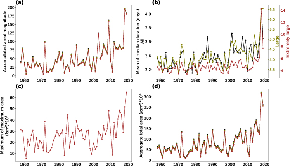
Figure 2. Observed temporal changes in the considered metrics ((a) accumulated areal magnitude, (b) mean of median duration, (c) maximum of maximum area, and (d) aggregate total area) of all (black line), large (olive line), and extremely large (brown line) contiguous heatwaves, respectively, during the period 1958–2020 across Australia.
Download figure:
Standard image High-resolution imageFigure 3 shows changes in the individual large and extremely large contiguous heatwaves during 1989/90–2019/20 compared to 1958/59–1988/89. We find that most contiguous heatwave metrics of extremely large heatwaves and the median duration of large heatwaves show a significant change in 1989/90–2019/20 relative to 1958/59–1988/89 (figure 3). This implies that extremely large heatwaves are growing larger and are lasting longer. Previous research on Australian heatwaves found that heatwaves in Australia are mainly driven by modes of natural climate variability, global warming, and synoptic systems (Pezza et al 2012, Perkins 2015). This suggests that the observed increase in extremely large heatwaves could be due to the combination of climate variability, global warming, and large and persistent synoptic systems. Further research is required to identify the causes behind the increase in extremely large contiguous heatwaves in recent decades compared to the past, which may consider investigating the influence of multidecadal climate variability (such as Interdecadal Pacific Oscillation (IPO)) and global warming on Australian contiguous heatwaves.

Figure 3. Probability distribution function (PDF) of considered metrics of large (a)–(d) and extremely large (e)–(h) contiguous heatwaves during the recent period (1989/90–2019/20; orange) and the earlier period (1958/59–1988/89). The KS test with bootstrapping is used to test for significant differences between the distributions, with the resulting p-value presented in the respective plots.
Download figure:
Standard image High-resolution image3.2. Influence of ENSO and IOD on large contiguous heatwaves in Australia
The larger interannual variability of all considered seasonal contiguous heatwave metrics is seen during 1958–2020 and is more pronounced during the recent decade (figure 2). Previous studies have linked variability in heatwave metrics to climate variability (Perkins-Kirkpatrick et al 2017). Hence, here we investigated the influence of natural climate variability modes (ENSO and IOD) on large and extremely large contiguous heatwaves. As previous studies suggested that ENSO and IOD interact with each other (Meyers et al 2007, Risbey et al 2009, Ummenhofer et al 2011), we consider co-occurring phases rather than individual phases for further analysis (see section 2.4). The CNRM-CM6-1 SMILE data provides a larger sample of co-occurring modes (table 1) relative to observations. We evaluated the performance of the CNRM-CM6-1 SMILE in simulating temporal variability of the seasonal contiguous heatwave metrics against the observations. Results suggested that the CNRM-CM6-1 SMILE is able to skilfully represent the temporal variability of the aggregate total area (figure 4), accumulated areal magnitude (figure S1), maximum of the maximum area (figure S2) and mean of median duration (figure S3) of contiguous heatwaves in Australia.
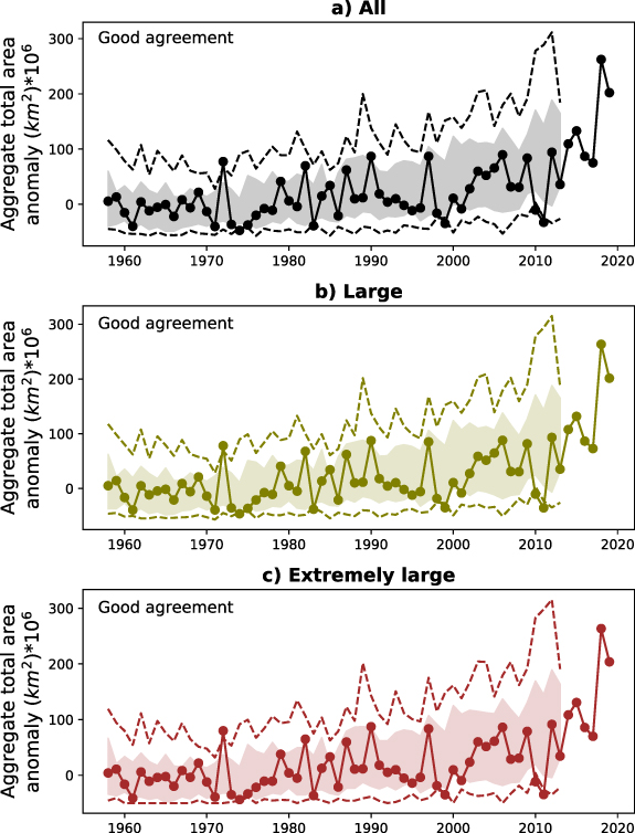
Figure 4. Comparison of observed (thick line) seasonal aggregate total area of (a) all, (b) large, and (c) extremely large contiguous heatwaves, respectively, with the CNRM-CM6-1 SMILE data (thin lines represent 0th and 100th percentile; shading indicate the 75th percentile range (i.e. 12.5th–87.5th percentile)).
Download figure:
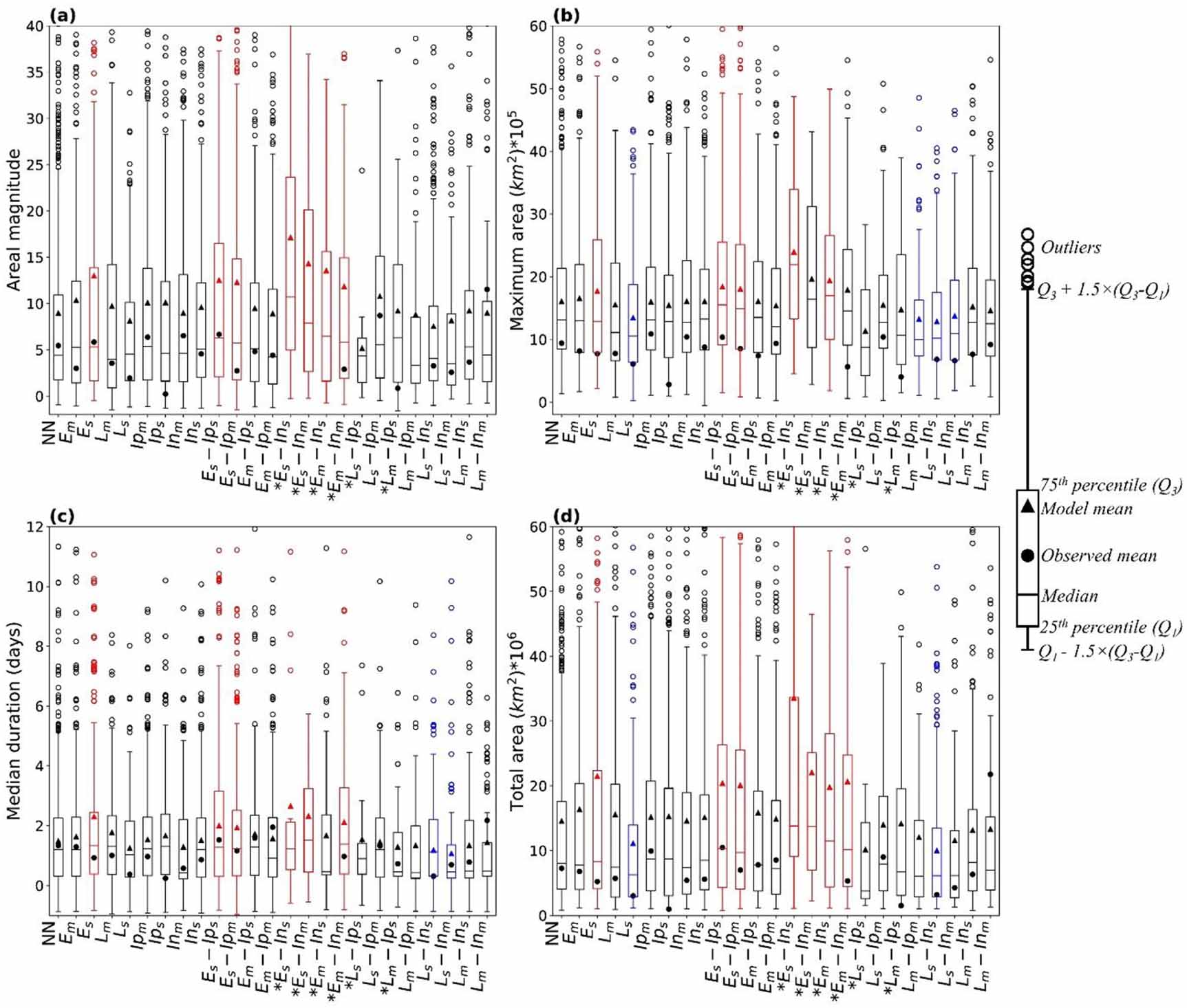
Standard image High-resolution imageFigures 5 and 6 show the variations of detrended contiguous heatwave metrics of large and extremely large events of co-occurring variability modes. The results obtained without detrending are presented in the supplementary figures S4 and S5. However, detrending the contiguous heatwave metrics had minimal effect on the results. Results suggest that areal magnitude, maximum area, total area, and median duration of both the large and extremely large contiguous heatwaves are significantly higher during the strong El Niño (Es), strong El Niño co-occurring with strong IOD positive (Es-Ips), and with moderate IOD positive (Es-Ipm) seasons relative to the neutral seasons (where both ENSO and IOD are in neutral phase; NN) (figures 5 and 6). This means that Es, Es-Ips, and Es-Ipm conditions significantly influence the increase in size (spatial extent) and duration (temporal length) of these events. These results are in line with those from previous studies, which found that El Niño seasons are associated with dry conditions, above-normal temperatures, and more heatwave days over much of Australia (Arblaster and Alexander 2012, Perkins et al 2015). In addition to El Niño seasons, the drier conditions are also observed during co-occurring El Niño and IOD positive seasons over many parts of Australia (Meyers et al 2007, Ummenhofer et al 2011). During these phases, the abnormally dry conditions caused by both of these phases likely favour heatwave conditions and thus result in significant increases in extremely large contiguous heatwaves.

Figure 5. The distributions of detrended metrics ((a) areal magnitude, (b) maximum area, (c) median duration, and (d) total area) of large contiguous heatwaves during seasons of various climate variability modes. Red and blue coloured box plots indicate significant increase and decrease, respectively, in the mean of the distribution of considered large contiguous heatwave metrics corresponding to various modes of climate variability relative to neutral conditions (NN) at a significance level of 0.05. Asterisk indicates limited sample data during certain modes of variability. The filled triangle and filled circle represent the mean of model data and the mean of observation data during the corresponding modes, respectively. Empty circles represent the outliers of model data.
Download figure:
Standard image High-resolution image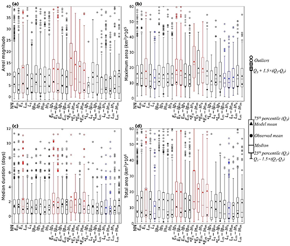
Figure 6. Same as figure 5 but for detrended extremely large contiguous heatwave metrics ((a) areal magnitude, (b) maximum area, (c) median duration, and (d) total area).
Download figure:
Standard image High-resolution imageThe co-occurring strong La Niña and strong IOD negative (Ls-Ins) seasons are associated with the most significant decrease in most of the considered metrics of the large and extremely large contiguous heatwaves compared to the NN seasons (figures 5 and 6). Both the La Niña and IOD negative modes are associated with below normal temperatures and enhanced rainfall conditions over many parts of Australia (Pepler et al 2014, Perkins et al 2015). Their interactions (La Niña and IOD negative) likely exacerbate wet conditions (Meyers et al 2007, Ummenhofer et al 2011), which are not favourable for heatwaves. Co-occurring modes such as strong El Niño with strong IOD negative (Es-Ins) and moderate IOD negative (Es-Inm), moderate El Niño with strong IOD negative (Em-Ins) and moderate IOD negative (Em-Inm) exhibit a significant association with some of the considered metrics of large and extremely large contiguous heatwaves compared to the NN conditions. However, there is a limited sample of data during these co-occurring modes (Es-Ins, Es-Inm, Em-Ins, and Em-Inm), and as such, these results might not be statistically robust. The observations and CNRM-CM6-1 SMILE data suggest that the combinations of El Niño co-occurring with IOD negative (Es-Ins, Es-Inm, Em-Ins, and Em-Inm) and La Niña with IOD positive (Ls-Ips and Ls-Ipm) occur very rarely, consistent with previous studies (Meyers et al 2007, Ummenhofer et al 2011).
Larger variability of heatwave metrics is seen across various co-occurring modes of ENSO and IOD, even when their mean values are significantly higher compared to the neutral conditions (figures 5 and 6). The high probability of occurrence of large and extremely large contiguous heatwaves, which cover massive areas, particularly during the Es, Es-Ips, and Es-Ipm seasons (table S1), results in a larger composite mean, even though relatively moderate events are also possible. Although the mean values of large and extremely large contiguous heatwave metrics are significantly lower during the Ls-Ins seasons compared to the neutral conditions, there is a (low) probability for the occurrence of those events with a massive area (table S1). This significant decrease in their composite mean during the Ls-Ins seasons is likely due to the low (high) probability of occurrence of large and extremely large contiguous heatwaves which cover massive (moderate) areas (table S1).
3.3. Physical mechanisms
The above-presented results show that large and extremely large contiguous heatwaves in Australia are significantly increasing (decreasing) during the Es, Es-Ips, and Es-Ipm (Ls-Ins) conditions. To examine the large-scale underlying physical mechanisms associated with these phases, we calculated the composite differences of detrended MSLP and geopotential height at 500 hPa (z500) between these phases and the neutral phase. This composite analysis provides more insights into how the Es, Es-Ips, Es-Ipm, and Ls-Ins phases influence contiguous heatwaves in Australia.
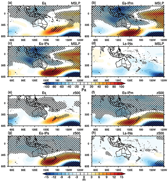
The composite maps of MSLP and z500 during the Es, Es-Ips, Es-Ipm, and Ls-Ins are shown in figure 7. The composite difference patterns of MSLP are similar with z500 during the Es, Es-Ips, and Es-Ipm, and Ls-Ins phases. The Es, Es-Ips, and Es-Ipm phases show positive changes in MSLP and z500 along the Southeast of Australia over the Tasman Sea and negative changes along the northwest of Australia over the Indian Ocean (figure 7). These positive and negative changes of MSLP and z500 are significant, particularly during the Es-Ips, and Es-Ipm phases. No significant changes of MSLP and z500 are observed during the Ls-Ins phase. The zonal pressure dipole-like circulation features such as low-pressure cyclonic circulation over the northwest and high-pressure anticyclonic circulation over the southeast of Australia observed during the Es, Es-Ips, and Es-Ipm phases favour the persistence of blocking highs over the Tasman Sea (Pezza et al 2012, Boschat et al 2015). The blocking of high-pressure systems over the Tasman Sea favours the development and amplification of heatwaves over Australia (Pezza et al 2012, Perkins et al 2015). Hence, the increased geopotential height and the pressure dipole-like circulation features near Australia associated with the Es, Es-Ips, and Es-Ipm phases influence the contiguous heatwaves in Australia.
Figure 7. Composite differences of detrended mean sea level pressure (MSLP) (a)–(d) and geopotential height at 500 hPa (z500) (e)–(h) between Es, Es-Ips, Es-Ipm, and Ls-Ins phases and NN phase, respectively. Hatching indicates significance at the 0.05 level. The statistical significance is tested with permutation test.
Download figure:
Standard image High-resolution image
3.4. Implications and limitations
The results presented here have a number of important implications for Australian industry and society. The increase in extremely large contiguous heatwaves coupled with prolonged duration (figure 3) results in simultaneous exposure of crops to heatwaves over large connected regions. The prolonged exposure of crops to heatwaves can decrease their productivity (Asseng et al 2011). The intensification of the areal magnitude of extremely large contiguous heatwaves (figure 3) will also expose a greater proportion of the Australian population to intense heatwaves in neighbourhood regions at the same time. Severe heatwaves seriously affect human health (Hanna et al 2011) and have a negative impact on the emergency health services (Lindstrom et al 2013) and electricity supply systems (McEvoy et al 2012). Many previous studies investigated the effects of heatwaves (not necessarily contiguous) on Australian society (Hanna et al 2011, Lindstrom et al 2013), but there is a lack of research on the impacts of large contiguous heatwaves on society. Further research is needed to consider and quantify the impacts of simultaneous exposure of regions to contiguous heatwaves.
There are a few caveats and limitations to this study that need to be highlighted. In this study, the spatial connectivity of heatwaves is only allowed for those grid cells with adjacent land area, which omits Tasmania from contiguous events on the mainland. Moreover, we have only considered ENSO and IOD and their interactions but not the SAM, which also influences heatwave characteristics over southern parts of Australia (Perkins et al 2015). Nevertheless, this study is the first to systematically quantify observed changes in spatial characteristics of contiguous heatwaves in Australia during the historical period and comprehensively investigate their association with the interactions of ENSO and IOD. Our results will help understand how the contiguous heatwaves in Australia respond to ENSO and IOD and their interactions. An enhanced understanding of the interactive influence of ENSO and IOD on contiguous heatwaves can help improve the seasonal prediction skill of contiguous heatwaves.
4. Conclusions
Contiguous heatwaves are growing in terms of their spatial and temporal extent and occurring with higher intensity across Australia during 1958–2020. Results highlight that metrics of extremely large contiguous heatwaves in Australia have significantly increased during 1989/90–2019/20 compared to 1958/59–1988/89. Further research on future projected changes in contiguous heatwaves across Australia utilising the various emission scenarios is required to develop a comprehensive heatwave hazard management plan. Strong El Niño (Es), strong El Niño co-occurring with strong IOD positive (Es-Ips), and with moderate IOD positive (Es-Ipm) modes of climate variability leads to the significant increase in all the considered metrics of large and extremely large contiguous heatwaves relative to the neutral (ENSO neutral + IOD neutral; NN) conditions. These phases (Es, Es-Ips, and Es-Ipm) are associated with the anomalous pressure dipole-like circulation patterns near Australia (anticyclonic pressure anomaly over the Tasman Sea and cyclonic pressure anomaly along the northwest Australia over the Indian ocean), which provides the favourable environment for the heatwaves. While strong La Niña with strong IOD negative (Ls-Ins) promotes a significant decrease in most of the considered large and extremely large contiguous heatwave metrics compared to the NN mode. These results provide insights into the underlying physical mechanisms of contiguous heatwaves in Australia and may help improve forecasts of contiguous heatwaves through incorporation of predictions of ENSO and IOD interactions. Further, future studies may consider investigating how ENSO and IOD interact with other large-scale drivers (such as SAM, the IPO and the Madden-Julian Oscillation) and how their interactions influence contiguous heatwaves in Australia. Such studies will provide a more comprehensive understanding of the driving mechanisms of contiguous heatwaves in Australia.
Acknowledgments
The authors thank CSIRO and the Bureau of Meteorology for providing the AWAP gridded dataset. We thank the U. K. Hadley Centre for making available HadISST data and the NCI for its computational assistance. The authors thank CNRM/CERFACS modelling group for producing and making available CNRM-CM6-1 model data. S E Perkins-Kirkpatrick is supported by ARC Grant (FT170100106) and CLEX Grant (CE170100023).
Data availability statement
The data that support the findings of this study are openly available at the following URL/DOI: https://esgf-node.llnl.gov/search/cmip6/.