Reanalysis-driven simulations may overestimate persistent contrail formation by 100%–250%

We use radiosonde data from the IGRA V2 from 2012 to 2016 [38, 39]. The soundings are generated from 2788 stations globally, 1081 of which contribute between 2012 and 2016. The instruments used in each sounding can vary depending on year and country. To be consistent, we include only those stations using the Vaisala RS92 sensor. This choice is a compromise between the need for a widely used sensor, to ensure sufficient coverage, and for accurate readings. The RS92 is used at 360 of the 1081 contributing stations (see figure S1 (available online at stacks.iop.org/ERL/17/014045/mmedia)). This sensor has also been shown to measure temperature and relative humidity—the two critical measurements for contrail formation and persistence—to within $\pm 1$ K and 10%, respectively [40, 41]. The RS92 sensor is known to have a daytime dry bias due to a radiation error of around 30% at 10 km and 50% at 15 km for humidity [42]. Information on the sensors used by the stations is available from the World Meteorological Organization (WMO) [43]. Vaisala, the manufacturer of the RS92 sensor, incorporates a proprietary correction for these factors, which leads to similar corrections as developed by Dirksen et al [41]. These corrections are applied prior to them being received by the IGRA and so are included in our analysis.

Trent et al [32] also compared RS92 sonde data from the UK Met Office (UKMO) with readings at standard and significant pressure levels to humidity profiles from the AIRS. First, a time lag and humidity correction was applied to the RS92 sonde data. This was compared to the AIRS data as well as data from the global climate observing system (GCOS) reference upper air network (GRUAN), who supply high resolution, bias corrected, radiosonde data but for fewer locations than the UKMO. These results found the satellite data to be drier than the corrected sonde data by 21.74% at 250–300 hPa and smaller differences at lower altitudes. In comparison, the satellite data and GRUAN data differed by only 0.24% at 250–300 hPa, with a maximum difference at 500–600 hPa of 5.7%.

The number of RS92 sonde launches for each station between 2012 and 2016 is shown in figure S1. These 360 stations launched 930 091 sondes ('profiles') in this period. Observations with not-a-number (NaN) readings for pressure, temperature or dewpoint depression were removed. Profiles where the vertical distance between observations is greater than 3 km or where all observations are below 12 km are removed. These two requirements account for 14.7% of profiles and our results use the remaining 793 044.

The distribution of stations and profiles varies by latitude band, as seen in figure 1. Forty-eight percent of profiles are in 30° N–60° N. The number of profiles increases by 9.8% from 2012 to 2016 and varies by up to 13% between seasons. By latitude, the distribution of profiles is skewed towards the northern hemisphere, representing 75% of profiles, with the fewest profiles in the Antarctic (2.0%) and southern mid-latitudes (6.5%). This distribution is similar to that of aviation fuel burn, where 92% is burned in the northern hemisphere [44]. Finally, 54% of the sondes are launched during the day, with this proportion increasing from 53.6% in 2012 to 54.6% in 2016. Sondes are typically released twice a day at noon and midnight. This is reflected in the IGRA data where 98.5% of sondes are launched at 3 h intervals (i.e. 3 AM UTC, 6 AM UTC etc.), matching the output time of both sets of reanalysis data.

Zoom In Zoom Out Reset image size

The selected locations of sondes are not uniformly distributed globally. This means that they may not be representative of the overall meteorological conditions. To assess whether they are representative for the purposes of the PCC distribution, figures S2 and S3 show the percentage PCC in the northern mid-latitudes for DJF and JJA comparing the sonde data with collocated ERA5 profiles, all ERA5 profiles in the given latitude band and season, and all ERA5 profiles on land locations also in the given latitude band and season. The mean cruise-altitude PCC in DJF is 10% lower than the data at sonde locations for ERA5 and 12% lower for MERRA-2. In comparison, in JJA, the mean cruise-altitude PCC is 46% higher than the value for ERA5 and 34% higher for MERRA-2. This suggests a seasonal bias in how representative the sonde data is for persistent contrail formation. Using land locations only does not explain the differences between the reanalysis data at sonde versus all locations.

Humidity measurements in the sonde data are provided as a dew point depression ($T - {T_d}$), which measures the difference between the ambient temperature, $T$, and the dew point temperature, ${T_d}$. The dew point temperature measures the temperature to which air must be cooled to become saturated with respect to water. The dew point temperature can be converted to the water vapor partial pressure by

$$\begin{align}{p_{{\text{wv}}}} = a{ }{e^{\dfrac{{b{T_d}}}{{c + {T_d}}}}},\end{align} \tag{ 1 }$$

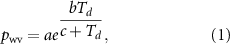
where ${p_{{\text{wv}}}}$ is the water vapor partial pressure, and $a = 611.2$ Pa, $b = 17.67$ K⁻¹, and $c = 243.5$ K are fitted coefficients [45]. This is converted to a relative humidity by estimating the saturation water vapor partial pressure by

$$\begin{align} p_{{\text{wv}}}^{{\text{sat}}}= 100{ }{{\text{e}}^{\frac{{ - 6096.9385}}{T} + 16.635794 - 0.02711193T + 1.673952 \times {{10}^{ - 5}}{ }{T^2} + 2.433501log\left( T \right)}},\end{align} \tag{ 2 }$$

where $p_{{\text{wv}}}^{{\text{sat}}}$ is the saturation water vapor partial pressure and $T$ is the ambient temperature [46].

We estimate altitude using pressure data. Each data point is considered to represent a layer with constant temperature its lower to upper edge. A layer is defined by the geometric mid-point between consecutive observations. The barometric formula with constant temperature is used to estimate the difference in altitude between the layer edges. The altitude is initialized assuming the highest recorded pressure value is at the surface. We therefore calculate

$$\begin{equation}{z_ + } = {z_ - } + \frac{{RT}}{{gM}}log\left( {\frac{{{p_ - }}}{{{p_ + }}}} \right),\end{equation} \tag{ 3 }$$

where ${z_ + }$ and ${z_ - }$ are the altitude of the upper and lower edge of the layer respectively, $R = 8.31$ J (mol K)⁻¹ is the universal gas constant, $g = 9.81$ m s⁻¹ is the gravitational acceleration at the surface of the Earth, $M = 0.028$ kg mol⁻¹ is the average molecular mass of air, and ${p_ + }$ and ${p_ - }$ are the pressure of the upper and lower edge of the layer, respectively.

Two reanalysis datasets are tested in this paper: the MERRA-2 [15] and the ECMWF ERA5 [18]. The reanalysis data are generated from data-assimilation models that combine numerical simulations with a wide range of atmospheric observations.

MERRA-2 is generated from the Goddard Earth Observation System model, version 5 and is the latest reanalysis product from the Global Modeling and Assimilation Office (GMAO). MERRA-2 uses a cube-sphere horizontal discretization with a resolution of around 0.5$^\circ\, \times$ 0.625$^\circ$ (∼50 km) and 72 hybrid-eta levels from surface to 0.1 hPa. For this study, the three-hourly, 0.5$^\circ\, \times$ 0.625$^\circ$, 72-layer data was used. Humidity data is assimilated using the normalized pseudorelative humidity and a complete set of the data assimilated is provided in the literature [17]. MERRA-2 assimilates radiosonde and other water vapor observations up to 300 hPa since the accuracy of radiosonde water vapor observations at lower pressures is lower [25].

ERA5 is the second global reanalysis data studied. It is based on four-dimensional variational (4D-Var) data assimilation using Cycle 41r2 of the Integrated Forecasting System. ERA5 is a spectral model at the TL639 resolution (∼31 km) with 137 layers to 1 hPa. The hourly 0.25$^\circ\, \times$ 0.25$^\circ$ data on 37 fixed pressure levels was used, provided from the Copernicus Data Store (CDS). ERA5 assimilates radiosonde and other water vapor observations until the diagnosed tropopause at ∼300 hPa [25].

Radiosonde profiles are collocated to the same time and locations based on the sonde release data. Additional temporal or spatial location information as the sonde rises is not provided in the sonde data. The grid-average values are used from both ERA5 and MERRA-2 and we retain all vertical layers from ground to the highest for which observations are available for each individual profile.

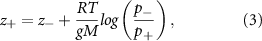
The GRUAN provides state-of-the-art, high quality humidity measurements from radiosondes [41]. These measurements use the RS92 sensor, but are corrected for time-lag, radiation dry bias, and other errors. Detailed uncertainty estimates are also provided. The GRUAN only provides data for 32 locations and thus cannot be used to study global trends like the IGRA. The accuracy and uncertainty data is used as a benchmark to compare to IGRA and reanalysis data. In this section, we provide an overview of how uncertainties in temperature and humidity are propagated to the PCC.

The GRUAN separates uncertainties in temperature and humidity measurements (including corrections) according to whether they are correlated or uncorrelated. A method to combine uncertainties across several observations in a given profile is provided [47]. The uncertainty of the average conditions across $M$ observations for each profile, $l$, is calculated by

$$\begin{equation}\begin{gathered} \overline{{k_{i,l}}} = \frac{\mathop\sum \limits_{j = i - M}^{j = i + M}{k_{i + j,l}}}{2M}\hfill \\ \overline{{r_{i,l}}} = \frac{\sqrt{\mathop\sum\limits_{j = i - M}^{j = i + M} r_{i + j,l}^2}}{2M}\hfill \\ \end{gathered},\end{equation} \tag{ 4 }$$

where ${k_{i + j}}$ and ${r_{i + j}}$ represent the (perfectly) correlated and uncorrelated uncertainties at observation $i + j$, respectively, and $2M$ represents a normalizing factor, such that. In this case all weights are equal. Each observation's uncertainty is calculated using data provided in each GRUAN dataset.

The combined uncertainty of the average signal of profile $l$, $\overline {\left( {{u_{i,l}}} \right)}$, is

$$\begin{equation}\overline {{u_{i,l}}} = \sqrt {{{\overline {{k_{i,l}}} }^2} + {{\overline {{r_{i,l}}} }^2}} .\end{equation} \tag{ 5 }$$

We must now combine uncertainties across multiple profiles with observations in the same layer. We assume that $\overline {\left( {{u_{i,l}}} \right)}$ is independent and uncorrelated across profiles, allowing us to calculate the combined uncertainty, $\widehat {\left( {{u_i}} \right)}$, using quadrature by

$$\begin{equation}\widehat {{u_i}} = \frac{1}{N}\sqrt {\sum\limits_{l = 1}^N {{\overline {{u_{i,l}}} }^2}} .\end{equation} \tag{ 6 }$$

To propagate uncertainties in temperature and relative humidity for the PCC, we can define the PCC in terms of four auxiliary variables, ${X_i}$, that all must be greater than zero as

$$\begin{equation}{\text{PCC}} = \prod\limits_{i = 1}^3 \left[ {\left[ {{X_i} > 0} \right]} \right],\end{equation} \tag{ 7 }$$

where $\left[ {\left[ \ldots \right]} \right]$ is the Iverson brackets, which maps the statement within to its possible values (e.g. true when ${X_i} > 0$, false otherwise). Each condition follows the PCC definition defined as

$$\begin{align} {X_1}\left( {T,p} \right) & = {T_c}\left( p \right) - T \nonumber\\ {X_2}\left( {{\text{RH}},T,p} \right) & = {\text{RH}} - {\text{R}}{{\text{H}}_c}\left( {T,p} \right) \nonumber\\ {X_3}\left( {RH,T} \right) & = RH\dfrac{{p_{{\text{wv}}}^{{\text{sat}}}\left( T \right)}}{{p_{{\text{ice}}}^{{\text{sat}}}\left( T \right)}} - 1 .\end{align} \tag{ 8 }$$

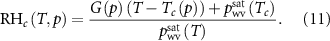
${T_c}\left( p \right)$ is defined as [48]

$$\begin{align}{T_c}\left( p \right) & = 226.69 + 9.43\ln \left( {G\left( p \right) - 0.053} \right) \nonumber\\ & \quad + 0.72\ln {\left( {G\left( p \right) - 0.053} \right)^2},\end{align} \tag{ 9 }$$

where $G\left( p \right)$ is the gradient of the mixing between the ambient air and engine exhaust conditions on the temperature-water vapor partial pressure curve. It is defined as

$$\begin{equation}G\left( P \right) = \frac{{{\text{EI}}\left( {{\text{H}_2}\text{O}} \right){c_p}p}}{{0.622{\text{ LHV}}\left( {1 - {\eta _0}} \right)}}.\end{equation} \tag{ 10 }$$

${\text{R}}{{\text{H}}_c}\left( {T,p} \right)$ is defined as

$$\begin{equation}{\text{R}}{{\text{H}}_c}\left( {T,p} \right) = \frac{{G\left( p \right)\left( {T - {T_c}\left( p \right)} \right) + p_{{\text{wv}}}^{{\text{sat}}}\left( {{T_c}} \right)}}{{p_{{\text{wv}}}^{{\text{sat}}}\left( T \right)}}.\end{equation} \tag{ 11 }$$

Assuming each measured variable is randomly distributed with mean value ${\mu _\varepsilon }$ and uncertainty $\sigma _\varepsilon ^2$, and uncorrelated with each other, then the combined uncertainty is modeled as

$$\begin{equation}{\mathrm{X}_i}\sim \mathcal{N}\left( {{\mu_{\mathrm{X}_i}},\sigma _{{\mathrm{X}_i}}^2} \right),\end{equation} \tag{ 12 }$$

where the variance is found by

$$\begin{equation}\sigma _{{\mathrm{X_i}}}^2 = \sum\limits_{j = 1}^m {\left( {\frac{{\partial {X_i}}}{{\partial {\varepsilon _j}}}} \right)^2}\sigma _{{\varepsilon _j}}^2.\end{equation} \tag{ 13 }$$

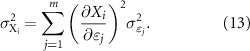
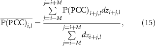
This also assumes that $T$ and ${\text{RH}}$ are uncorrelated with each other. While we do expect these variables to be correlated, the GRUAN does not provide information on the correlation coefficient between the $T$ and ${\text{RH}}$ uncertainties. The probability of PCC is then found by

$$\begin{equation}\mathbb{P}\left( {{\text{PCC}}} \right) = \mathop \prod \limits_{i = 1}^4 \mathbb{P}\left( {{X_i} > 0} \right) = \mathop \prod \limits_{i = 1}^4 \phi \left( {\frac{{{\mu _{{X_i}}}}}{{{\sigma _{{X_i}}}}}} \right),\end{equation} \tag{ 14 }$$

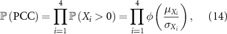
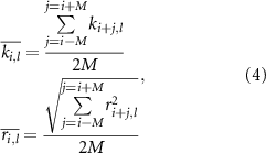
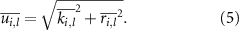
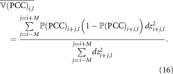
where $\mathbb{P}$ is the notation used for probability and φ is the cumulative distribution function of the normal distribution. Assuming each estimate of $\mathbb{P}\left( {{\text{PCC}}} \right)$ is independent, we can estimate the proportion of a layer that satisfies the PCC by

$$\begin{equation}\overline {\mathbb{P}{{\left( {{\text{PCC}}} \right)}_{i,l}}} = \frac{\mathop \sum \limits_{j = i - M}^{j = i + M} \mathbb{P}{\left( {{\text{PCC}}} \right)_{i + j,l}}d{z_{i + j,l}}}{\mathop \sum \limits_{j = i - M}^{j = i + M} d{z_{i + j,l}}},\end{equation} \tag{ 15 }$$

where $d{z_{i + j,l}}$ is the distance between the mid-point of the given observation and adjacent observations. The variance of this distribution is

$$\begin{align}& \overline {\mathbb{V}{{\left( {{\text{PCC}}} \right)}_{i,l}}}\nonumber\\ & \quad = \frac{\sum\limits_{j = i - M}^{j = i + M} \mathbb{P}{\left( {{\text{PCC}}} \right)_{i + j,l}}\left( {1 - \mathbb{P}{{\left( {{\text{PCC}}} \right)}_{i + j,l}}} \right)dz_{i + j,l}^2}{\sum\limits_{j = i - M}^{j = i + M}dz_{i + j,l}^2}.\end{align} \tag{ 16 }$$

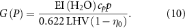
To quantify the probability of contrail formation and persistence, we define the PCC. The PCC identifies whether a contrail could form and persist in the local conditions if an aircraft passed. Satisfying the PCC means satisfying three conditions: (a) the air must be supersaturated with respect to ice (${\text{R}}{{\text{H}}_i} > 100\%$); (b) the relative humidity with respect to water must be above the critical ambient relative humidity with respect to water (${\text{R}}{{\text{H}}_w} > {\text{R}}{{\text{H}}_{w,{ }C}}$); and (c) the relative humidity with respect to water must be below 100% (${\text{R}}{{\text{H}}_w} < 100\%$).

${\text{R}}{{\text{H}}_i}$ is calculated by

$$\begin{equation}{\text{R}}{{\text{H}}_i} = {\text{R}}{{\text{H}}_w}\frac{{p_{{\text{wv}}}^{{\text{sat}}}}}{{p_{{\text{ice}}}^{{\text{sat}}}}}{ },\end{equation} \tag{ 17 }$$

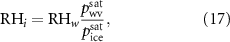
where ${\text{R}}{{\text{H}}_w}$ is the measured relative humidity with respect to water, and $p_{{\text{ice}}}^{{\text{sat}}}$ is the estimated saturated partial pressure with respect to ice. This is approximated by [46]

$$\begin{equation}p_{{\text{ice}}}^{{\text{sat}}} = 100{ }{{\text{e}}^{\frac{{ - 6024.5282}}{T} + 24.721994 + 1.0613868 {{10}^{ - 2}}T - 1.3198825 {{10}^{ - 5}} {T^2} - 0.49382577{\text{log}}\left( T \right)}}{ },\end{equation} \tag{ 18 }$$

where $T$ is the local, measured air temperature in kelvin. The ${\text{R}}{{\text{H}}_{w,{ }C}}$ is calculated using equation (10). Here, ${\eta _{\text{o}}}$ is equal to the propulsive efficiency (${\eta _{\text{p}}}$) multiplied by the thermal efficiency (${\eta _{\text{t}}}$). While fuel and ambient air properties are relatively fixed globally and for each aircraft, ${\eta _{\text{o}}}$ can vary by 10–15 percentage points depending on engine technology and mode of operation [49]. We assume ${\eta _{\text{o}}} = 0.35$ as a mid-point between currently used engines as well as new engines that have recently entered the market. Prior studies [50] have estimated ${\eta _{\text{o}}} = 0.31$ for the year 2006 using the Base of Aircraft Data (BADA) dataset [51].

Multiplying the PCC at a given altitude (averaged over time) by the likelihood of a flight passing through that altitude gives a metric of the frequency with which contrails will form at the location. For a given vertical profile, we can use the vertical distribution of aviation fuel burn as a proxy for the likelihood that an aircraft will be present at that altitude. Accordingly, we calculate the fuel-burn weighted PCC, ${F_{{\text{PCC}}}}$, at any given time $t$ by

$$\begin{equation}{F_{{\text{PCC}}}} = \frac{{{{\mathop \smallint \nolimits }}{P_{{\text{PCC}}}}\left( z \right)F\left( z \right){\text{d}}z}}{{{{\mathop \smallint \nolimits }}F\left( z \right){\text{d}}z}},\end{equation} \tag{ 19 }$$

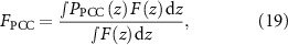
where ${P_{{\text{PCC}}}}\left( z \right)$ is the proportion of space-time that satisfies the PCC, $F\left( z \right)$ is the fuel burn profile, and $z$ is the vertical coordinate. ${F_{{\text{PCC}}}}$ thus represents the proportion of the vertical fuel burn profile in a region that could lead to a persistent contrail forming. It is calculated from the Aviation Environmental Design Tool (AEDT) [44] fuel burn inventory for 2015. We use a global, annual average value as aviation fuel burn varies by less than 25% between summer and winter [52]. The vertical profile is also not expected to change significantly between seasons or within the latitude bands considered.

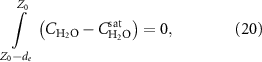
The final metric used is the evaporation depth, ${d_e}$, which measures the depth below a specific altitude at which the area between the water concentration and ice saturation concentration profile is zero. For this paper, we specify the initial altitude, ${Z_0}$, to be 10 km. It is calculated by solving the equation

$$\begin{equation}\int\limits_{{Z_0} - {d_e}}^{{Z_0}} \left( {{C_{{{\text{H}}_{\text{2}}}{\text{O}}}} - C_{{{\text{H}}_{\text{2}}}{\text{O}}}^{{\text{sat}}}} \right) = 0,\end{equation} \tag{ 20 }$$

where ${C_{{{\text{H}}_{\text{2}}}{\text{O}}}}$ is the water vapor concentration and $C_{{{\text{H}}_{\text{2}}}{\text{O}}}^{{\text{sat}}}$ represents the saturation water vapor concentration.

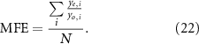
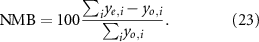
Throughout this paper, we use a range of error metrics including the mean absolute error (MAE), mean factor error (MFE), normalized mean bias (NMB), and correlation coefficient (R²). The MAE is calculated by

$$\begin{equation}{\text{MAE}} = \frac{\sum\limits_i \left| {{y_{o,i}} - { }{y_{e,{ }i}}} \right|}{N},\end{equation} \tag{ 21 }$$

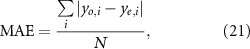
where ${y_o}$ represents the observation from the sonde data and ${y_e}$ represents the estimate from the reanalysis data, with N observations. The MFE is calculated by

$$\begin{equation}{\text{MFE}} = \frac{\sum\limits_i \frac{{{y_{e,i}}}}{{{y_{o,i}}}}}{N}.\end{equation} \tag{ 22 }$$

Finally, the NMB is calculated by

$$\begin{equation}{\text{NMB}} = 100{ }\frac{{{{\mathop \sum \nolimits }}_i{y_{e,i}} - {y_{o,i}}}}{{{{\mathop \sum \nolimits }}_i{y_{o,i}}}}.\end{equation} \tag{ 23 }$$

Studies [12, 28, 30, 53, 54] have analyzed observations of ISS regions, providing information on potential regions where contrails could persist. The proportion of the vertical profile that is ISS by latitude is shown in figures 2(a)–(c), with typical cruise altitude (9–12 km) shaded in gray on each panel. Sonde observations from the IGRA show that the altitude where the percentage of ISS regions peaks increases towards the equator. At the same time, the peak value decreases by 65% from the Arctic to the tropics. At typical cruise altitudes, the percentage PCC varies by less than 5% across latitude bands in the sonde observations. In comparison, the percentage PCC varies by 31% across latitude bands in ERA5 and 48% in MERRA-2. Both sets of reanalysis data also overestimate the average percentage PCC at cruise altitudes. In the northern mid-latitudes, where 62% of aviation fuel is burned, ERA5 overestimates this by 43% and MERRA-2 by 137%.

Zoom In Zoom Out Reset image size

The proportion of the vertical profile that satisfies the PCC is shown in figures 2(d)–(f), aggregated into three latitude bands. The mean cruise-altitude PCC is overestimated in both reanalyses by a factor of 1.3–3.5. This bias factor is highest in the mid-latitudes, at 2.0 for ERA5 and 3.5 for MERRA-2, and lowest in the Arctic, at 1.3 and 1.8, respectively. Given that the PCC overestimate changes with latitude, simulations of contrail forcing using these reanalyses likely also include a latitude-dependent bias. These biases also vary with altitude and could result in additional errors when estimating the effects of future supersonic aircraft in the tropics, which are expected to cruise at altitudes between 15 km and 20 km [55].

Sonde observations show that the mean PCC-weighted altitude decreases towards the poles, from 14 km in the tropics (0°–30° N) to 8.1 km in the Arctic (60°–90° N). This decrease is reproduced by ERA5 and MERRA-2. In the tropics, ERA5 overestimates the mean PCC-weighted altitude by 430 m, while MERRA-2 underestimates it by 410 m. In the Arctic, ERA5 overestimates the mean PCC-weighted altitude by 590 m and MERRA-2 underestimates it by 322 m. Seasonal differences and other analyses are shown in figure S8.

We also include the percentage ISS and PCC estimated using the sonde observations from the GRUAN in gray for the northern mid-latitudes (figures 2(b) and (c)). For the percentage ISS, despite the locations not being collocated, the IGRA and GRUAN data match within 10% between 6 km and 12 km. For the PCC, a consistent offset of around one percentage point is found between the IGRA and GRUAN up to 12 km, with a greater IGRA underestimate above this. We also include the ISS and PCC for the ERA5 and MERRA-2 data at the GRUAN sonde launch locations in the faded red and blue, respectively. These results show that the GRUAN-collocated ERA5 data overestimates the GRUAN mean cruise altitude ISS by a factor of 1.4, consistent with the IGRA data. The mean cruise altitude PCC from ERA5 shows a lower overestimate of a factor of 1.7 when using the GRUAN data. For MERRA-2, the mean cruise altitude ISS and PCC is overestimated by a factor of 2.1 and 2.4.

Our results suggest that the reanalysis datasets overestimate humidity in PCC regions relative to sonde-based measurements. Radiosondes are not the only possible ground truth, but satellite-based estimates have been found to report either similar or lower humidities at these altitudes compared to sonde-based measurements [32]. To draw stronger conclusions would require a co-located comparison of reanalysis estimates of PCC regions against satellite measurements, which is outside the scope of this study.

We also quantify the variation in these errors by season. Previous studies have found that contrails are twice as likely to form in the winter than the summer, despite only 22% of annual air traffic occurring during the northern hemispheric winter [56]. Figure 3 shows how the observed and simulated PCC profiles vary between northern hemisphere winter (DJF) and summer (JJA) for the northern mid-latitudes, covering 62% of global aviation fuel burn.

Zoom In Zoom Out Reset image size

Based on sonde data, differences in the vertical PCC profile are dominated by changes that occur between 5 and 11 km. Above 11 km, the percentage PCC is roughly the same across seasons, with a 24% reduction from DJF to JJA at 11 km. However, between 5 and 11 km, the mean percentage PCC is a factor of 4.1 greater in DJF than in JJA. The shape of the profile within the cruise altitude region also changes. In DJF, the peak PCC probability occurs below 9 km, and decreases with increasing altitude. In JJA, the peak instead occurs at 11 km. Combined, these differences result in a mean cruise-altitude PCC proportion during DJF, which is three times greater than during JJA. This seasonal trend is also reflected in contrail observation studies [57, 58].

Meteorological reanalysis data qualitatively reproduce observed seasonal variations in overall PCC probability. However, both ERA5 and MERRA-2 overestimate the mean cruise-altitude PCC. ERA5 overestimates this by a factor of 2.0 across both seasons. MERRA-2 shows an overestimate of a factor of 3.4 and 3.6 in DJF and JJA, respectively. Both reanalysis models also overestimate the increase in the mean PCC altitude from DJF to JJA. The sonde data show a 7.6% increase while in ERA5 and MERRA-2, we find a 19% and 14% increase, respectively.

We use the fuel-burn weighted PCC to produce a single metric that accounts for the altitude of aviation fuel burn and that can be compared between locations. This metric measures the percentage of aviation fuel burn that could lead to the formation of a persistent contrail. The variation of fuel-burn weighted PCC over the full 2012–2016 period is shown in figure 4 for each latitude band. The correlation coefficient (R²), mean absolute error (MAE), and normalized mean bias (NMB) are calculated between each reanalysis data time series and the sonde data and are provided in the legend. The R² is used to assess whether temporal variations in fuel-burn weighted PCC are well-represented in the reanalysis data. MAE indicates how far from the 'true' PCC occurrence the average reanalysis estimate is, while NMB indicates whether the reanalysis overestimates (NMB > 0) or underestimates (NMB < 0) the likelihood of formation. Each time series is a daily average of all fuel-burn weighted PCC.

Zoom In Zoom Out Reset image size

For all latitudes, the reanalysis data overestimates the fuel-burn weighted PCC. The greatest NMB occurs at mid-latitudes, where 62% of aviation fuel is burned. ERA5 shows a bias of 44%, while MERRA-2 has a bias that is a factor of 3.1 greater. Both sets of reanalysis data show a positive bias in the tropics and Arctic. For ERA5, this bias is 9% and 8%, respectively. In comparison, for MERRA-2, the bias is 126% in the tropics and 38% in the Arctic.

MERRA-2 has an R² of 0.55 in the tropics and 0.93 in the Arctic. This suggests that, notwithstanding the NMB, MERRA-2 captures a large fraction of the seasonal variability in persistent contrail formation. ERA5 is also able to capture the seasonal variability with an R² of 0.52 in the tropics and 0.86 in the Arctic.

We also quantify the effect of engine overall efficiency (${\eta _{\text{o}}}$) on the fuel-burn weighted PCC (figure S6). Increasing ${\eta _{\text{o}}}$ is expected to lead to an increase in the potential for contrail formation [15]. In the sonde data, we find that an increase in ${\eta _{\text{o}}}$ from 0.30 to 0.40 causes the fuel-burn weighted PCC to increase by approximately 9.4%. This increase in fuel-burn weighted PCC varies with time between a maximum of 14% and minimum of 5.8%. The sensitivity to efficiency is similar in ERA5 and MERRA-2, with a mean increase in fuel-burn weighted PCC of 11% and 9.8%, respectively. Both sets of reanalysis data exhibit a larger variability over the five-year period studied, with the percentage change in fuel-burn weighted PCC varying between 4.4%–26% for MERRA-2 and 6.2%–21% for ERA5. This could lead to unexpectedly strong seasonal or latitudinal variations in contrail simulations using reanalysis data that would not be reproduced in reality.

The average fuel-burn weighted PCC for each latitude band and season are shown in figure 5, with the MFE (see equation (22)) shown in the legend. MERRA-2 overestimates the fuel-burn weighted PCC in all cases, while ERA5 overestimates in all but two cases (0°–30° S in DJF and 60°–90° S in JJA). In addition, the MFE is higher for MERRA-2 than ERA5 in all cases except 60°S—90°S. Finally, the MFE is greatest for ERA5 and second greatest for MERRA-2 in the northern mid-latitudes, where 62% of fuel is burned.

Zoom In Zoom Out Reset image size

Contrail lifetime is determined by several factors. A contributing factor is the time taken for contrail ice crystals to fall into subsaturated air and evaporate. Initially, ice crystals fall and grow in supersaturated conditions until the relative humidity with respect to ice, ${\text{R}}{{\text{H}}_i} = 100\%$. Upon reaching subsaturated conditions, they lose ice mass until the surrounding air reaches an ${\text{R}}{{\text{H}}_i} = 100\%$. As they continue falling in subsaturated conditions, they will lose more ice mass until they evaporate. The distance fallen before evaporation (the 'evaporation depth') is a contributor to contrail lifetime and can be estimated from the background relative humidity profile (see section 2).

Figure 6 shows how the mean evaporation depth for regions satisfying the PCC at 10 km varies from 2012 to 2016. The sonde data shows a mean depth of 1.3 km, varying between a minimum of 1.0 km in northern hemisphere summer and maximum of 1.8 km in northern hemisphere winter. Comparing with reanalysis data, ERA5 has a NMB of 17% and a MAE of 0.2 km, which is smaller than MERRA-2 (45% and 0.6 km, respectively). The contrail lifetime estimated using ERA5 is thus likely to be more accurate than when using MERRA-2, although an overestimate would be expected from both. Both sets of reanalysis data predict a similar, positive R², suggesting that seasonal variations are well represented. This suggests that the reanalysis models predict the vertical gradients in temperature and water vapor correctly.

Zoom In Zoom Out Reset image size

Figure S7 shows a time series of the median and interquartile range (IQR) of the evaporation depth for the sonde data and each data assimilation system. The IQR provides information on the ability of the reanalyses to represent 'deep' supersaturation regions (upper quartile) or 'shallow' regions (lower quartile), and the skew in the distribution. These results follow those discussed for the mean evaporation depth except for two differences. Firstly, the distribution of evaporation depth is skewed by a small number of relatively large evaporation depths, exceeding 5 km in 3.9% of cases. This causes the mean evaporation depth to be ∼0.5 km greater than the median. These cases are important as they may contribute to longer lasting and larger contrails that can have a greater impact [36]. Secondly, both ERA5 and MERRA-2 do not capture the strength of the seasonal cycle in the median evaporation depth. The observations vary by a factor of 2.2 between a maximum of 1.3 km in JJA and minimum of 0.6 km in DJF. In comparison, ERA5 varies from 1.4 km in JJA to 1.0 km in DJF, a factor of 1.4 seasonality, and MERRA-2 varies from 1.9 km in JJA to 1.2 km in DJF, a factor of 1.6 seasonality. This means that contrail lifetimes may not increase as much in the northern hemisphere summer as would be expected from the sonde data.

Contrail studies have shown that in-flight, operational strategies to divert flights around PCC or ISS regions may reduce the number of contrails that form [13, 59, 60]. These strategies rely upon forecasts being accurate enough to predict PCC regions. To assess this, we compare individual observations of PCC regions with estimates from the reanalysis data. ERA5 and MERRA-2 correctly predict PCC regions (true positives) 13% and 52% of the time, respectively, between 9 and 12 km globally. In comparison, non-PCC regions (true negatives) are correctly predicted 95% and 93% of the time, respectively (see tables S1 and S2). The results are similar to recent comparisons between aircraft observations and ERA5, where ice supersaturation is found to be correctly predicted 18% of the time [61]. These results suggest that testing mitigation strategies on historical data may not be accurate since individual contrail-forming regions cannot be identified with sufficient reliability [13, 59, 62–65]. Similar issues will affect forecast data, presenting a challenge for practical contrail mitigation.

We also assess whether the ability of reanalysis data to predict individual PCC regions is driven by errors in temperature or humidity by swapping either the temperature or humidity profiles in sonde data with that in the reanalysis data. Figure S11 shows the improvement on various metrics of swapping temperature or humidity for both ERA5 and MERRA-2 in the northern mid-latitudes, between 9 and 12 km. For both ERA5 and MERRA-2, swapping the temperature profile has a small effect, improving the number of true positives by 2 and 1 percentage points, respectively. In comparison, swapping the humidity profiles leads to a 54 and 28% points improvement. This confirms that errors in humidity are driving the difference between the sonde and reanalysis estimates of percentage PCC [66]. The remaining difference may be due to the lower vertical resolution of the reanalysis compared with the sonde data.

We find four central results. Firstly, both ERA5 and MERRA-2 overestimate the percentage PCC across latitude bands. In the northern mid-latitudes, where 62% of jet fuel is burned, the mean percentage PCC at cruise altitudes is overestimated by a factor of 2.0 and 3.5, respectively, for ERA5 and MERRA-2. Similar biases are also found in the tropics and Arctic.

Secondly, the sonde data exhibits seasonality in PCC in the mid-latitudes, where the mean cruise percentage PCC is a factor of 1.7 higher in DJF than JJA. MERRA-2 consistently overestimates this mean cruise PCC by a factor of 3.4–3.6 and ERA5 by a factor of 2.0. Both sets of reanalysis data correctly predict the seasonality in PCC, which is important to capture as studies suggest contrails forming in the winter are expected to have a disproportionate climate impact [56]. This extends results showing that reanalysis data are unable to identify the formation or persistence of contrails in comparison to using atmospheric measurements from aircraft [61].

Thirdly, the evaporation depth, a proxy for contrail lifetime, is overestimated by 45% in MERRA-2 and 17% in ERA5. This suggests that simulations using MERRA-2 and ERA5 would predict contrails surviving to lower depths than expected from observations and, thus, with longer lifetimes. However, the evaporation depth only captures the effect of ice crystal sedimentation. Synoptic-scale influence on contrail lifetime is not captured [67].

Finally, both reanalyses are unable to identify individual PCC regions. At cruise altitudes, MERRA-2 correctly predicts PCC regions 52% of the time, while ERA5 correctly predicts 13% of these. This suggests that mitigation strategies focusing on avoiding specific contrails using solely model output may not be practical given the inability of reanalysis data and, by extension, forecasts in predicting individual PCC regions. Sensitivity tests show that improvements to reanalysis data should focus on estimating humidity more accurately to improve individual PCC estimates.

These findings come with some caveats. First, the relative measurement uncertainty of the RS92 humidity sensor is ∼10% [41]; however, our findings show biases in the reanalysis data that are greater than this. The RS92 sensor also has a daytime dry relative bias due to radiative heating that is ∼30% at 10 km and ∼50% at 15 km [44–47]. This dry bias can explain some differences between sonde and reanalysis data. To test the robustness of our findings, we compared 2877 profiles from the GCOS GRUAN, which corrects raw RS92 measurements for time lag and radiation bias. Figure S13 shows that the GRUAN data predicts a 4.2% occurrence of PCC regions between 9 and 12 km. The IGRA data underestimates the occurrence of PCC regions by 24% relative to the GRUAN data, while MERRA-2 and ERA5 show a factor of 2.5 and 1.6 overestimates, respectively. For comparison, the 95% confidence interval in the mean occurrence of PCC regions at cruise altitudes in the GRUAN data is 3.7%–4.6%. We are unable to apply the GRUAN corrections to IGRA as the data is not stored at the original time resolution, which is required for both the time lag and radiative heating issues. In addition to the PCC, figure S14 compares the GRUAN and IGRA temperature below 250 K and the relative humidity between 10% and 95%. These results show a correlation of 0.996 and 0.90, respectively, with a mean percentage bias of −0.06% and −6%, respectively. Further work would benefit if the data could be acquired at the original time resolution.

Second, this bias also cannot explain spatial and temporal differences between the sources. In addition, the comparison between the sonde and reanalysis data are based on the grid average. We do not interpolate the reanalysis data in either time or space. As a result, PCC regions smaller than an individual layer will not be resolved, but this should have no effect on the ability to resolve deeper PCC regions. We also do not study the effects of spatial resolution, which could influence the ability to identify PCC regions. Third, the IGRA data does not include the location of the sonde data as it traverses vertically and so we are unable to account for the advection of an individual sonde through its profile. This could change the performance of the reanalysis data, and location information should be included in future stores of the observations. Finally, as shown in figures S2 and S3, the locations of the sonde data are not representative of the latitude bands studied. For this reason, the observations used do not represent the underlying percentage PCC of a given region, and additional observations, from sondes or other sources, would be required.

Reanalysis data are a vital tool in contrail modeling and other applications. Our results show biases in the predicted number of persistent contrails that could form using reanalysis data. The biases have shown that ERA5 and MERRA-2 both overestimate the probability of persistent contrail formation at cruise altitudes on average by a factor of 1.9 and 3.5, respectively, in the mid-latitudes. Furthermore, both sets of reanalysis data fail to capture variations in the probability and expected lifetime of contrails with season, altitude, and latitude, which cannot be accounted for with a single scalar correction. These results are consistent with comparisons of ice supersaturation between flight and reanalysis data, which have been shown to be weakly correlated [61]. Meteorological data that prioritizes the upper troposphere, lower stratosphere (UTLS) humidity coupled with direct observational estimates of contrail coverage and properties are needed to improve and better constrain current estimates of atmospheric conditions.