
Abstract
Persistent contrails are an important climate impact of aviation which could potentially be reduced by re-routing aircraft to avoid contrailing; however this generally increases both the flight length and its corresponding CO emissions. Here, we provide a simple framework to assess the trade-off between the climate impact of CO
 emissions and contrails for a single flight, in terms of the absolute global warming potential and absolute global temperature potential metrics for time horizons of 20, 50 and 100 years. We use the framework to illustrate the maximum extra distance (with no altitude changes) that can be added to a flight and still reduce its overall climate impact. Small aircraft can fly up to four times further to avoid contrailing than large aircraft. The results have a strong dependence on the applied metric and time horizon. Applying a conservative estimate of the uncertainty in the contrail radiative forcing and climate efficacy leads to a factor of 20 difference in the maximum extra distance that could be flown to avoid a contrail. The impact of re-routing on other climatically-important aviation emissions could also be considered in this framework.
Export citation and abstract BibTeX RIS

Content from this work may be used under the terms of the Creative Commons Attribution 3.0 licence. Any further distribution of this work must maintain attribution to the author(s) and the title of the work, journal citation and DOI.
1. Introduction
Persistent contrails are a climate impact of aviation whose radiative forcing may be comparable with that from aviation carbon dioxide (CO ) emissions (Burkhardt and Kärcher 2011). There are few viable technological options for reducing contrail formation (Haglind 2008, Gierens et al 2008), meaning that the easiest way of mitigating this climate impact is to avoid routing aircraft through regions where contrails can form. As the ice-supersaturated regions (ISSRs) where contrails form frequently occur in relatively shallow layers (Rädel and Shine 2007), much of the previous work in this area has concentrated on avoiding contrail formation by altitude changes (Williams et al 2002, Fichter et al 2005, Mannstein et al 2005, Rädel and Shine 2008, Schumann et al 2011, Deuber et al 2013). Reducing the cruise altitude of the entire global fleet of aircraft by 6 000 ft can substantially reduce contrail formation (Fichter et al 2005); however this requires aircraft to fly at a sub-optimal altitude, leading to an increase in fuel burn and CO
 emissions. Assessing the viability of such a strategy requires calculating the trade-off between CO
 emissions and contrails. Zou et al (2013) use a monetization approach, which involves making value judgements on the relative 'cost' of each climate impact. Deuber et al (2013) use climate metrics which are based on the response of the atmosphere to the relative forcings, providing a framework which is useful in a policy context. For an individual flight, however, a framework is required which can be adapted to take into account the characteristics of the aircraft and the prevailing weather conditions since the altitude at which contrails are formed is highly dependent on the weather pattern (Irvine et al 2012).
Moreover, less attention has been paid to re-routing aircraft without altitude changes; such a strategy might be preferable where the increase in flight distance is small, since it allows an aircraft to remain at the altitude where it is most fuel-efficient. As motivation for this approach we provide an idealised example. Figure 1 shows a circular ISSR of radius 2 degrees, located along the great circle route between two airports. As shown on figure 1 the shortest alternative route avoiding the ISSR (in zero wind conditions) is to fly great circle routes from LON-A, and A-NY. This increases the flight distance by 22.5 km, 0.4% of the original route. We note also that since the increase in flight distance is dependent on how wide the ISSR is in the direction perpendicular to the original flight, it is independent of the contrail length. Together this implies that if regions in which contrails may be formed can be predicted, and routes recalculated to avoid them, then the added flight distance and therefore the CO penalty may be small.
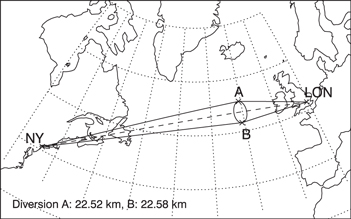
Figure 1. An illustration of typical distances added to a flight between New York (NY) and London (LON), in order to avoid an ISSR (ellipse) of radius 2 degrees. For flight in still air, the shortest route is the great-circle route (dashed line). The shortest alternative routes which avoid the ISSR (solid lines) are two great circle routes via point A or B.
Download figure:
Standard image High-resolution imageWe assess the following situation: at the flight planning stage, an aircraft is predicted to encounter an ISSR along its proposed route. An alternative route is found, at the same altitude, which avoids the ISSR but increases the flight length. Which route is preferable? Considering only the climate impact of the contrails and CO emissions (thus neglecting other non-CO
 emissions that have a climate effect such as oxides of nitrogen, NO
 ), the new route is preferable only if the climate impact of the CO
 emissions from flying the additional distance are smaller than the climate impact of the avoided contrail.
Towards answering this question, this work provides a simple framework with which to assess the trade-off between the climate impact of aviation CO emissions and contrails for a single flight. We show how this decision is impacted by uncertainties in the input parameters which result from the limitations of our current understanding of the climate impacts of aviation contrails. Here we assume that there has been a policy decision in favour of avoiding contrails where it would be climatically beneficial to do so, and show the results for a range of metrics and time horizons, to illustrate how different policy choices affect the decision of which route to take. This work provides a simple framework with which to interpret output from more complex calculations which simulate multiple flights in a realistic air-traffic framework (e.g. Sridar et al (2013)) with a larger range of aviation climate impacts (e.g. Grewe et al (2014)).
Section 2 provides details of the framework and the parameters used in the calculations. The framework is applied with representative figures for 'typical' contrails in section 3, and the sensitivity of the results to uncertainties in the input parameters is examined. Conclusions are presented in section 4.
2. The framework
It is only beneficial to fly extra distance  to avoid making a contrail, if the climate impact of the extra distance flown is smaller than the climate impact of the avoided contrail. There is therefore a distance for which these climate impacts are equal (discussed in terms of a turning-point by Deuber et al (2013)); this implies that it is beneficial to avoid making the contrail only if
  is smaller than this threshold distance,
  , which in the simple framework developed here is given by:

where the numerator is the climate impact of making the contrail, defined in terms of the contrail length  and width
  , and climate efficacy E. The denominator is the climate impact of the CO
 emissions from flying the additional distance to avoid making the contrail, defined in terms of the fuel flow FF in kg fuel per km and the emission index of CO
 ,
,  , which is a constant (3.16 kg CO
 (kg fuel)
 for kerosene fuel). The climate impact is measured by an emission metric M, applied with time horizon H. These parameters are discussed in turn in the following sections.
2.1. Contrail parameters
The contrail climate impact is related to the area covered by the contrail, expressed here as the product of its length and width. Here, we define  to be the distance travelled by the aircraft through an ISSR; therefore it is determined by the size of the ISSR and the path the aircraft takes through this. Data from MOZAIC (Measurements of Ozone and Water Vapour by Airbus In-Service Aircraft) show a peak path length of 150 km through ISSRs (Gierens and Spichtinger 2000), although ISSR sizes range from the order of 10 km to 1000 km (Gierens and Spichtinger 2000, Irvine et al 2013, Iwabuchi et al 2012). The eventual contrail width is determined by the lifetime of the contrail and the magnitude of the vertical wind shear, which acts to increase the effective horizontal cross-section of the contrail. Neither the contrail width or lifetime (required for the calculation of the climate metrics) are simple to pre-determine. The range of observed and modelled linear contrail widths is 1–10 km, generally with a peak at smaller values (Freudenthaler 1995, Duda et al 2004, Burkhardt and Kärcher 2009, Iwabuchi et al 2012). Contrail-cirrus lifetimes of up to 24 h have been observed (e.g. Haywood et al (2009)) but contrail lifetimes are generally not well-constrained by observations, particularly since long-lived contrails become difficult to track once they evolve into contrail-cirrus. Modelling of individual contrails suggests a modal lifetime of 1 h (Schumann 2012), and a typical duration of less than 6 h (Irvine et al 2014) based on air-parcel trajectories. We assume a contrail lifetime of 5 h in the climate metric calculations, following Fuglestvedt et al (2010). This lifetime has previously been used as an upper-bound for the lifetime of young contrails (Newinger and Burkhardt 2012). Measurements of a small number of short-lived contrails indicate that larger heavier aircraft may produce wider and thicker contrails than smaller lighter aircraft (Jeßberger et al 2013); given the lack of similar data for persistent contrails in ISSRs we assume contrail properties to be independent of aircraft type.
2.2. CO parameters

The amount of additional CO emissions is the product of the distance, the fuel flow and
  . FF varies depending on the aircraft type. Representative values of FF for different classes of aircraft (referred to as small, medium, large and very large jets) were calculated using the FAST model (Lee et al 2005), assuming for each aircraft type a loading of 70% and typical design weights and cruise altitudes. Values range from about 3 g m
 to 11 g m
 . Increasing the flight distance requires the aircraft to carry additional fuel, which increases the weight of the aircraft and thus also increases the fuel burn. In this study we neglect this second order effect.
Previous work (Sridar et al 2013, Zou et al 2013) indicates that in a realistic air-traffic scenario, the most effective way of reducing contrail formation for small increase in fuel burn is through a combination of horizontal re-routing with altitude changes. The framework presented here could be expanded to include altitude changes by incorporating a fuel penalty to account for the increase in fuel burn from flying at a sub-optimal altitude; this was beyond the scope of the present study.
2.3. Climate metric parameters
There is no uniquely suitable choice of metric to measure the climate impact of the contrail and CO emissions. Here we use both the the absolute global warming potential (AGWP) and absolute global temperature potential (AGTP) for pulse emissions (since we consider a single flight), calculated with a time horizon H of 20, 50 or 100 years. The AGWP and AGTP are both frequently-presented metrics (Myhre et al 2013), but the choice of which one is most appropriate (and which time horizon is most appropriate) depends on the context and on the aims of any climate mitigation policy. The GWP (e.g. Myhre et al (2013)) with a 100 year time horizon is used for deriving
  -equivalent emissions for a set of greenhouse gases under the Kyoto Protocol to the United Nations Framework Convention on Climate Change. The GTP (e.g. Shine et al (2007)) may be a more appropriate metric for a policy based on meeting specified temperature targets. The AGWP is the time-integrated radiative forcing following a pulse of either contrail formation or CO
 emission. For the long time horizons used here, the AGWP of the contrails is independent of the choice of time horizon, as the contrail will have totally disappeared by the time horizon. Note that the AGWP of a contrail is closely related to the concept of 'energy forcing' due to contrails introduced by Schumann et al (2012) and differs only in the choice of unit (see supplementary information). By contrast, the AGTP measures the temperature change at some future time after the pulse: the memory associated with the thermal inertia of the oceans means that the contrail AGTP does vary with time horizon. For both the AGWP and AGTP, the CO
 impulse-response function, that determines the longevity of the CO
 perturbation following the pulse emission, is taken from Joos et al (2013). Additionally, the AGTP requires the specification of an impulse-response function, representing the temperature response to the pulse emission—this introduces an added uncertainty, as this depends on the climate sensitivity and the uptake of heat by the ocean. We use the widely-adopted formulation of Boucher and Reddy (2008) (e.g. in Myhre et al (2013)), for these illustrative purposes. The values of M used in the baseline calculations are shown in table 1
.
perturbation following the pulse emission, is taken from Joos et al (2013). Additionally, the AGTP requires the specification of an impulse-response function, representing the temperature response to the pulse emission—this introduces an added uncertainty, as this depends on the climate sensitivity and the uptake of heat by the ocean. We use the widely-adopted formulation of Boucher and Reddy (2008) (e.g. in Myhre et al (2013)), for these illustrative purposes. The values of M used in the baseline calculations are shown in table 1
.
Table 1.
Specific forcing, AGTP and AGWP values for CO and contrails, for three different time horizons. For CO
 X is kg(
 ), for contrails X is
  .
.
AGTP K X
|
AGWP W m yr X yr X
|
||||||
|---|---|---|---|---|---|---|---|
| Emission | Specific forcing W m X X
|
20 yr | 50 yr | 100 yr | 20 yr | 50 yr | 100 yr |
CO
|
1.77e-15 a | 6.6e-16 | 5.6e-16 | 4.9e-16 | 2.5e-14 | 5.4e-14 | 9.3e-14 |
| contrails | 1.96e-8 | 8.9e-14 | 1.3e-14 | 9.2e-15 | 1.1e-11 | 1.1e-11 | 1.1e-11 |
aJoos et al (2013)
For the contrail climate impact we also take into account E. E measures the equilibrium surface temperature response, per unit radiative forcing, relative to that of CO (Ponater et al 2005). There are only two published estimates of E for contrails: 0.6 (Ponater et al 2005) and 0.31 (Rap et al 2010). Given the lack of consensus, for our baseline calculations we take E to be 1.0, and calculate the sensitivity of our results to these smaller values of E.
Contrail radiative forcing will vary according to, for example, the time of day, the natural cloud cover, contrail thickness (which may itself have a dependence on aircraft type) and the underlying surface. In an operational setting, this would need to be accounted for by calculating the contrail radiative forcing using a forecast model. However, estimates of contrail radiative forcings will vary by model, as was shown by Myhre et al (2009). For our baseline calculations we use a contrail specific radiative forcing estimated from the Myhre et al (2009) radiative forcing intercomparison study, where a global homogeneous contrail cover of 1% with an optical depth of 0.3 produced an annual mean all sky net radiative forcing of about 0.1 W  , but we examine the sensitivity to this value in section 3.
3. Results
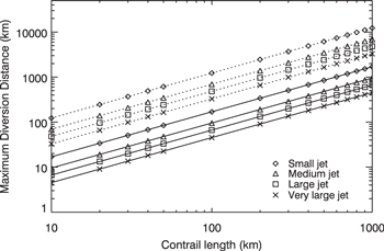
We investigate the results given by this simple framework for a range of aircraft types, using for these baseline calculations contrail parameters  = 1 km, E = 1.0 and a contrail lifetime of 5 h. Figure 2 shows
  calculated using these parameters for AGWP and AGTP metrics with H of 100 years. Since the total diversion distance
  is independent of contrail length, we calculate
  for contrail lengths between 10 km and 1000 km. To put the distances shown in figure 2 into context, the great circle distance between London and New York is 5541 km, and London and Singapore is 10 900 km. For a given aircraft type and metric,
  increases linearly with contrail length. Note that an alternative expression of the results is therefore as a factor of contrail length, i.e. using the 100 yr AGWP for a large jet,
  is 4.8 times the contrail length.
  shows some dependence on aircraft type, but the largest dependence is on the choice of metric.
Figure 2.
 as a function of contrail length for AGWP (dotted line) and AGTP (solid line) metrics for a time horizon of 100 years. The calculations use a contrail width of 1 km.
Download figure:
Standard image High-resolution image
The dependence of  on metric and time horizon is shown in table 2
for the case where
on metric and time horizon is shown in table 2
for the case where  = 100 km (results are shown rounded to the nearest 10 km). There is a large decrease in
  by increasing the time horizon from 20 to 50 years for the AGTP, but little difference between H of 50 and 100 years since the contrail is short-lived. The time dependence of the AGWP metric is solely due to the decay of the pulse of CO
 since the contrail AGWP is constant with time. To put these results into perspective, for the example in figure 1, if the contrail length was 100 km and
  was 22.5 km, then based on the results in table 1,
  is always greater than
  so it is climatically beneficial to fly the alternative route and avoid the contrail. Table 1 shows that for both metrics typically
  is four times larger for a small jet than for a very large jet (assuming the contrail properties are independent of aircraft type), indicating that longer diversions are possible for these smaller aircraft. The AGWP values are three to ten times greater than the AGTP, depending on time horizon, because the AGWP gives more weight to the shorter-lived forcing, while the AGTP has less memory of the short-lived forcing and thus gives more weight to the longer-lived CO
 forcing. This shows that the use of the AGWP means that it is perceived that longer diversions are possible than when using the AGTP.
Table 2.
 , for a contrail of length 100 km and width 1 km, for different aircraft classes as a function of climate metric and time horizon H.
| H (yr) | |||
|---|---|---|---|
| Aircraft class | 20 | 50 | 100 |
 (km) for AGTP (km) for AGTP |
|||
| Small jet | 1310 | 210 | 170 |
| Medium jet | 740 | 120 | 100 |
| Large jet | 510 | 80 | 70 |
| Very large jet | 350 | 50 | 50 |
 (km) for AGWP (km) for AGWP |
|||
| Small jet | 4530 | 2130 | 1230 |
| Medium jet | 2550 | 1200 | 690 |
| Large jet | 1780 | 840 | 480 |
| Very large jet | 1210 | 570 | 330 |
The impact of some of the uncertainties in our understanding of the contrail climate impact on the calculation of  are shown in table 3
, for a large jet forming a 100 km contrail with the climate impact assessed using the AGWP with H of 20 years and 100 years. First, using the same contrail specific RF, we assess the sensitivity to the choice of E. Since
are shown in table 3
, for a large jet forming a 100 km contrail with the climate impact assessed using the AGWP with H of 20 years and 100 years. First, using the same contrail specific RF, we assess the sensitivity to the choice of E. Since  scales linearly with E, the uncertainties in E lead to a factor of 3 difference between the highest and lowest E. To give a conservative estimate of the range of
  given possible values of E and contrail specific RF, high_E_SRF takes the high estimates of E and contrail specific RF and low_E_SRF takes low values. Note that the uncertainties in E and contrail specific RF are indicative of our current level of understanding and as such are not intended to give an upper and lower bound on
  . This gives a factor of 20 difference between the high and low estimates, changing
  from 3550 km to 170 km for H of 20 years.
Table 3.
The sensitivity of  to uncertainties in the contrail climate impact. Calculations are for a large jet forming a contrail of length 100 km and width 1 km, with the AGWP metric and H of 20 and 100 years.
| Calculation | Efficacy | Contrail SRF |  (km) for H (km) for H |
|
|---|---|---|---|---|
W m km km
|
20 yr | 100 yr | ||
| Baseline | 1.0 | 1.96e-8 | 1780 | 480 |
| Medium_E | 0.6 a | 1.96e-8 | 1070 | 290 |
| Low_E | 0.31 b | 1.96e-8 | 550 | 150 |
| high_E_SRF | 1.0 | 3.92e-8 c | 3550 | 970 |
| low_E_SRF | 0.31 | 6.09e-9 d | 170 | 50 |
aPonater et al (2005).
bRap et al (2010).
cCalculated from net RF 0.2 W  , Myhre et al (2009).
dCalculated from net RF 5.9 mW
, Myhre et al (2009).
dCalculated from net RF 5.9 mW  , Froemming et al (2011).
It is possible that in single events contrails or contrail cirrus may have a much larger radiative forcing than considered here. Haywood et al (2009) estimate the contrail specific forcing for a single observed contrail-cirrus event which is 1000 times larger than the values considered in table 3. This estimate, used to calculate  , gives
  on the order of 1 × 10
 km with H of 20 years, implying that aircraft should always divert to avoid contrails. Such extreme large values of contrail radiative forcing clearly increase the uncertainty on the value of
  , but do not change the general conclusion that there is often a climate benefit to avoiding contrail formation.
Thus far, the framework has assumed flight in still air (the fuel burn model and thus the calculation of FF assumes flight in still air). For flights which are predominantly east-west oriented, such as trans-Pacific or trans-Atlantic routes, the location of the jet stream strongly influences the route location (Irvine et al 2013). Re-routing the aircraft may route the aircraft into less favourable winds so that a smaller flight distance is achieved for the same fuel burn. We can incorporate the effect of a reduced tailwind into equation (1) via an additional parameter which increases FF by a factor  , where v is the true airspeed of the aircraft and
  is the change in speed induced by the effective tailwind. As a realistic upper bound on
  we calculate the horizontal wind shear in the region of the midlatitude jet stream, where we would expect to find the strongest horizontal gradients in wind speed at aircraft cruise altitudes. Based on the climatological latitudinal jet stream profile in the north Atlantic, calculated from 1989–2010 ERA-Interim data (Dee et al 2011), an aircraft flying eastbound with a diversion of 2 degrees from the jet core results in a reduced tailwind by 10 m s
 . Using v = 250 m
  , typical of a very large aircraft, decreases
  from 1210 km to 1160 km (for AGWP20, 100 km contrail), and from 330 km to 320 km (for AGWP100, 100 km contrail) when the effective headwind is added. Thus the effect of wind is much smaller than the effect of uncertainties in the calculation of the contrail climate impact.
4. Conclusions
We have developed a simple framework to enable the trade-off between contrail and CO climate impacts to be estimated for a single flight. The framework currently considers re-routing without altitude changes, which has the advantage of allowing the aircraft to fly at its most fuel-efficient altitude. The trade-off calculation depends on aircraft parameters such as fuel flow rate which are known a priori, and meteorological parameters such as the contrail size, lifetime and radiative forcing, which would be required to be known a priori were such a strategy to be implemented operationally.
The framework calculates the maximum extra distance that can be added to a flight, before the additional CO emissions outweigh the benefit of not contrailing. As the quantity of CO
 emissions depends on aircraft type, any decision to avoid making the contrail would be highly dependent on aircraft type. For example, using the AGWP metric with 100 year time horizon, the extra distance that a small jet can fly is more than ten times the avoided contrail length, whilst for a very large jet this reduces to three times. As discussed by Deuber et al (2013), it is important to choose a suitable metric, depending on the required outcome. Here, we find a factor of 3–10 difference between the AGTP and AGWP results, depending on the time horizon used.
This framework is useful to show where the major uncertainties are. Joos et al (2013) find that calculations of the atmospheric CO response agree within 15%, thus the climate impact of the flightʼs CO
 emissions can be calculated with a relatively small uncertainty, given knowledge of aircraft fuel burn. The calculation of the climate impact of the contrail has a much larger uncertainty. The uncertainty chiefly arises from two sources: an inability to estimate, a priori, the eventual size and therefore climate impact of the contrail that would be formed, and second the radiative forcing (which has a potential dependence on the time of day, not taken into account here) and climate efficacy of that forcing. Even if the radiative forcing were calculated operationally within a forecast model, there would still be an uncertainty in the size of the calculated radiative forcing due to the radiative forcing codes (Myhre et al 2009), and also due to uncertainty in the contrail characteristics. Taking into account the uncertainty in the eventual climate impact of a contrail of 100 km length, the estimate of the maximum diversion distance varies by a factor of 20.
The application of such a strategy in the real world would require highly accurate forecasts of ISSRs where potential contrails form, and the ability to know a priori the climate impact of a potential contrail, as well as being highly dependent on air traffic control and other operational and economic considerations. In addition, the overall climate impact of the flight should take into account the chemical forcings from aircraft  emissions; detailed calculations of such 'climate optimal' routings are currently being performed by the REACT4C project. We note here that for small horizontal diversions it is possible that the chemical forcings between the two routes would be comparable; however since the impact depends on where the
  emissions are advected, small diversions could potentially result in large differences in impact (Grewe et al 2014). The impact of black carbon and other aerosol emissions may also be important and could be incorporated in more detailed estimates (Jacobson et al 2012).
Nevertheless, despite the uncertainties, the calculations presented here indicate that once a metric (and time horizon) choice has been made, guidance can be given as to whether it is beneficial to divert to avoid contrails. So for example, adding 100 km distance to a flight to avoid making a contrail would seem beneficial for many of the cases presented here, and other parameter choices, such as the extreme high values in Haywood et al (2009), could allow significantly longer diversions.
Acknowledgments
The authors wish to acknowledge helpful discussions with Bethan Owen and David Lee and for providing data from the FAST model. We acknowledge Jan Fuglestvedt for providing helpful comments on an earlier draft of this paper, and two reviewers for their suggestions. This work is part of the REACT4C project, funded under the EU 7th framework programme, grant ACP8-GA-2009-233772.